A Black Box Doubly Fed Wind Turbine Electromechanical Transient Structured Model Fault Ride-Through Control Identification Method Based on Measured Data

Abstract

With the increasing proportion of grid-connected capacity of new energy units, such as wind power and photovoltaics, accurately constructing simulation models of these units is of great significance to the study of new power systems. However, the actual control strategies and parameters of many new energy units are often unavailable due to factors like outdated equipment or commercial confidentiality. This unavailability creates modeling challenges that compromise accuracy, ultimately affecting grid-connected power generation performance. Aiming at the problem of accurate modeling of fault ride-through control of new energy turbine “black box” controllers, this paper proposes an accurate identification method of fault ride-through control characteristics of doubly fed wind turbines based on hardware-in-the-loop testing. Firstly, according to the domestic and international new energy turbine fault ride-through standards, the fault ride-through segmentation control characteristics are summarized, and a general structured model for fault ride-through segmentation control of doubly fed wind turbines is constructed; Secondly, based on the measured hardware-in-the-loop data of the doubly fed wind turbine black box controller, the method of data segmentation preprocessing and structured model identification of the doubly fed wind turbine is proposed by utilizing statistical modal features and genetic Newton’s algorithm, and a set of generalized software simulation platforms for parameter identification is developed by combining Matlab and BPA; lastly, using the measured data of the doubly fed wind turbine in the black box and the software platform, the validity and accuracy of the proposed parameter identification method and software are tested in the simulation. Finally, the effectiveness and accuracy of the proposed parameter identification method and software are simulated and tested by using the measured data of black box doubly fed wind turbine and the software platform. The results show that the method proposed in this paper has higher recognition accuracy and stronger robustness, and the recognition error is reduced by 2.89% compared with the traditional method, which is of high value for engineering applications.

1. Introduction

In recent years, the global energy sector has continued to grow rapidly. According to the statistics of the International Renewable Energy Agency (IRENA), as of the end of 2023, the total global installed capacity of renewable energy has reached 337 million kilowatts, accounting for 30% of the total global installed power generation capacity, with a compound annual growth rate of 9.3% over the past 10 years. It is expected that the total installed capacity of the world will exceed 1.1 billion kilowatts by 2030 [1]. However, the large-scale grid integration of new energy sources has also brought a series of technical challenges to the power system: its volatility and intermittency have led to frequent grid frequency and voltage stability problems, the increasingly severe phenomenon of low-voltage or high-voltage off-grid, and the coupling of power electronic equipment with synchronous systems has triggered broadband oscillation problems [2,3,4,5,6]. These problems have triggered major grid accidents several times around the world. For example, a localized grid collapse triggered by a large-scale wind power off-grid in Northwest China in 2019 resulted in a power outage of several hours [7], and wind and photovoltaic (PV) power crises were exacerbated by a large-scale off-grid due to insufficient low-voltage ride-through capability during a winter storm in Texas, USA, in 2021 [8]. To address these technical challenges, accurate simulation analysis is necessary, and valid conclusions from simulation analysis rely on accurate modeling of new energy sources. For example, inaccurate LVRT modeling can affect the validation of relay protection algorithms, potentially leading to the misoperation of actual protection devices and triggering chain failures [9,10,11]. Therefore, to address the accurate modeling problems of the new energy “black box” controller fault ride-through control, this paper conducts related research, aiming to improve the accuracy and applicability of the new energy model, thereby providing theoretical support for the safe and stable operation of the new power system.

For a long time, scholars around the world have conducted numerous studies on wind power, photovoltaics, and energy storage power generation system models, gaining a deeper understanding of their related model structures and operational principles. For example, Hu et al. [12] and Tang et al. [13] ignored the current control process and modeled the amplitude-phase dynamics of the DFIG wind power system under DC voltage and rotor speed time scales, respectively. Jin et al. [14] established the equivalent impedance model of the DFIG wind power system and grid based on the impedance analysis method, which is used to analyze the interaction between the wind power grid-connected system and the grid. El-Shimy et al. [15] proposed a reduced-order model of a PV power system for small-signal stability assessment and estimated the maximum penetration level of the PV system. This study emphasized the importance of simplified models in power system stability analysis. Ning et al. [16] developed a Norton equivalent model for PV power systems and analyzed the effects of grid-connected capacity and grid strength on system resonance. Yonezawa et al. [17] developed a detailed and averaged model of a large-scale PV power system for electromagnetic transient simulation under grid faults. The model can accurately reflect the dynamic behavior of the PV system, but it has high computational complexity. Zhang et al. [18] proposes a composite demand-side simplified model structure containing loads, distributed PV generation, and energy storage systems and proposes a model parameter identification method based on environmental signals and fault data. The model structure is capable of recognizing the dynamic characteristics of PV generation and energy storage systems at the high-voltage bus by simplifying these systems. Fan et al. [19] proposes a simplification algorithm based on equivalent circuit modeling for large-scale battery packs, which can significantly improve simulation speed while maintaining accuracy, considering inconsistencies. However, most of the above studies have simplified or abstracted the models for different problems modeled in a particular scenario, which facilitates the analysis of the problem but, at the same time, reduces the accuracy of the model. In addition, existing studies also lack in-depth research on the modeling methods of new energy systems that take into account different fault control characteristics. In reality, when different types of short-circuit faults occur in the power grid, the new energy units tend to exhibit different control characteristics, i.e., the control objectives, control structures, control parameters, and control instructions of the unit control system will change with the fault changes to make the units exhibit different dynamic response characteristics [20,21].

In terms of model control parameter calibration, the transient control structure and parameters of the inverter, as the core component of the new energy power generation system, determine the transient response characteristics of the new energy during fault. However, the control structure and the parameters of the inverter in the new energy unit are usually complex to obtain directly due to changes in the operating environment and the black box nature of the actual controller. Therefore, it is necessary to estimate the unknown links in the model by combining the system identification method. System identification encompasses two key aspects: system structure identification and system parameter identification. For the system model structure, this paper selects a general model that can satisfy various calculation functions, such as tidal current calculation, transient stability simulation calculation, short-circuit calculation, and small disturbance stability calculation, among others. This model also features a variety of different decoupling control strategies. The parameter identification of the system is primarily divided into traditional identification methods and artificial intelligence identification methods [22]. Among them, the traditional identification method obtains the control parameters of the model through dynamic fitting methods, including the least squares method, theoretical analysis method, and frequency domain analysis method, among others. Kong et al. [23] proposes a two-stage parameter identification method for a direct-drive wind turbine converter dual closed-loop control system. A power step command is used to identify the control parameters based on the current response, employing the damped least squares method. Takahashi et al. [24] proposes a recursive least squares sensorless identification method for online identification of permanent magnet synchronous generator parameters, which can effectively detect feature changes during aging and degradation. Zhang et al. [25] proposed a new decoupled weighted recursive least squares (DWRLS) method, which improves the modeling accuracy by estimating fast and slow dynamic parameters separately. Xia et al. [26] improves the parameter discrimination accuracy of state-of-charge (SOC) estimation models for battery management systems based on the forgetting factor recursive least squares method.

The traditional identification methods are generally only applicable to the identification of linear systems, and they are difficult to apply to the identification of nonlinear systems. To address this issue, artificial intelligence (AI)-based identification methods have been proposed in the literature. These AI methods are intelligent techniques to identify model parameters by simulating human intelligence, automatic reasoning, learning, and searching, with strong problem-solving ability, and are not subject to the constraints of nonlinear links. Thus, they are more suitable for new energy systems that have high dimensionality of variables, strong coupling, and highly nonlinearized characteristics. Standard artificial intelligence algorithms include, for example, genetic algorithms, particle swarm optimization, differential evolution, and the JAYA algorithm, among others. Wu et al. [27] proposed a PMSM parameter identification method based on an improved cuckoo search algorithm. Yang-Wu et al. [28] proposed a genetic algorithm (GA)-based method for PMSG model parameter identification. Gao et al. [29] proposed an improved pollination algorithm for identifying the parameters of PMSM. Leng et al. [30] introduced a PSO algorithm based on chaotic mapping and Gaussian perturbation for parameter identification of PMSG motors. However, these optimization methods suffer from slow convergence, easy premature convergence, and low identification accuracy [31,32]. To address these problems, Yang et al. [33] proposed a Grey Wolf Optimizer (GWO) algorithm with an information-sharing search strategy to solve the parameter identification problem of doubly fed converters. In [34], a chaotic adaptive search GWO algorithm is proposed to recognize the parameters of PMSM. Liu et al. [35] proposed a parameter estimation method for the PMSM drive system based on an improved particle swarm algorithm to solve the parameter estimation model of the PMSM drive system. Wu et al. [36] indicates that the traditional photovoltaic cell model parameter identification method has several shortcomings, including low accuracy, slow convergence speed, and a high risk of falling into local optima. Therefore, this study proposes a photovoltaic cell model parameter identification method that improves upon the elephant swarm optimization algorithm. Han et al. [37] proposed a parameter identification method based on an atomic search algorithm; the experimental results demonstrate that the algorithm exhibits high accuracy and a fast convergence speed, achieving better results in PV cell model parameter identification. Yang et al. [38] In order to accurately identify the circuit model parameters, an improved optimization algorithm based on particle swarm optimization is used, which combines the optimization strategies and hybrid algorithms proposed in recent years to make up for the fact that the traditional particle swarm algorithm tends to get stuck in the local optimal solution. The efficiency of the multidimensional search is reduced.

In summary, although the new energy transient model parameter identification has achieved some research results, there are still the following difficulties:

(1) The new energy unit “black box” controller fault traversal characteristics are complex, linear and nonlinear coupling is strong, parameter identification is difficult, identification results are poorly adapted, and accuracy is low.

(2) The dynamic response of new energy units under symmetrical and asymmetrical fault types, different operating conditions, and various high and low voltage ride-throughs exhibits significant differences and shows strong sequential consistency. Its control strategy and parameters are diverse and intensive, with low identification efficiency.

(3) The fault ride-through control mechanism of the new energy unit “black box” controller is unknown, and equivalent modeling is difficult;

To solve these problems, the main contributions of this paper can be summarized as follows:

(1) A new energy unit “black box” controller fault traversal parameter identification method based on the genetic Newton algorithm is proposed, which can accurately identify the actual doubly fed wind turbine control strategy and parameters under symmetrical/asymmetrical fault types, different operating conditions, and different high and low voltage traversals.

(2) A segmentation method for the fault-crossing process based on statistical modal characteristics is proposed to divide the data interval of the fault stage accurately, and a general structured model framework for fault-crossing segmentation control of doubly fed wind turbines is constructed.

(3) A genetic Newtonian hybrid fault traversal parameter optimization algorithm is proposed, which combines global search and local optimization to improve accuracy and robustness significantly.

(4) Based on the proposed method and theory, a set of generalized black box new energy unit parameter identification software is developed by combining Matlab App Designer Version: 9.11.0.1769968 (R2021b) and PSD-BPA version 3.1. The proposed method and the developed software are validated using semi-physical hardware-in-the-loop test data from the RTLAB-based doubly fed unit. The results demonstrate that the proposed method is more accurate and robust, achieving a 2.89% reduction in error compared to the traditional method, which is of significant value for engineering applications. Meanwhile, the developed parameter identification software platform automates the entire process of data preprocessing, parameter optimization, and simulation verification, improving modeling efficiency by 40% and addressing the issue of convenience in engineering applications.

The structure of this paper is as follows:

Part I: Based on the new energy scale statistics of the International Renewable Energy Agency (IRENA), we point out the key grid integration technical challenges facing the global new energy development and emphasize that high-precision new energy modeling is the theoretical cornerstone of the security and stability analysis of new power systems. By systematically combing the research progress of wind power, photovoltaic and energy storage modeling, and combining it with the comparative analysis of the optimization performance of various identification algorithms, the current technological bottlenecks and methodological limitations are further clarified, thus laying an important theoretical foundation and research basis for the innovative solutions proposed in this study.

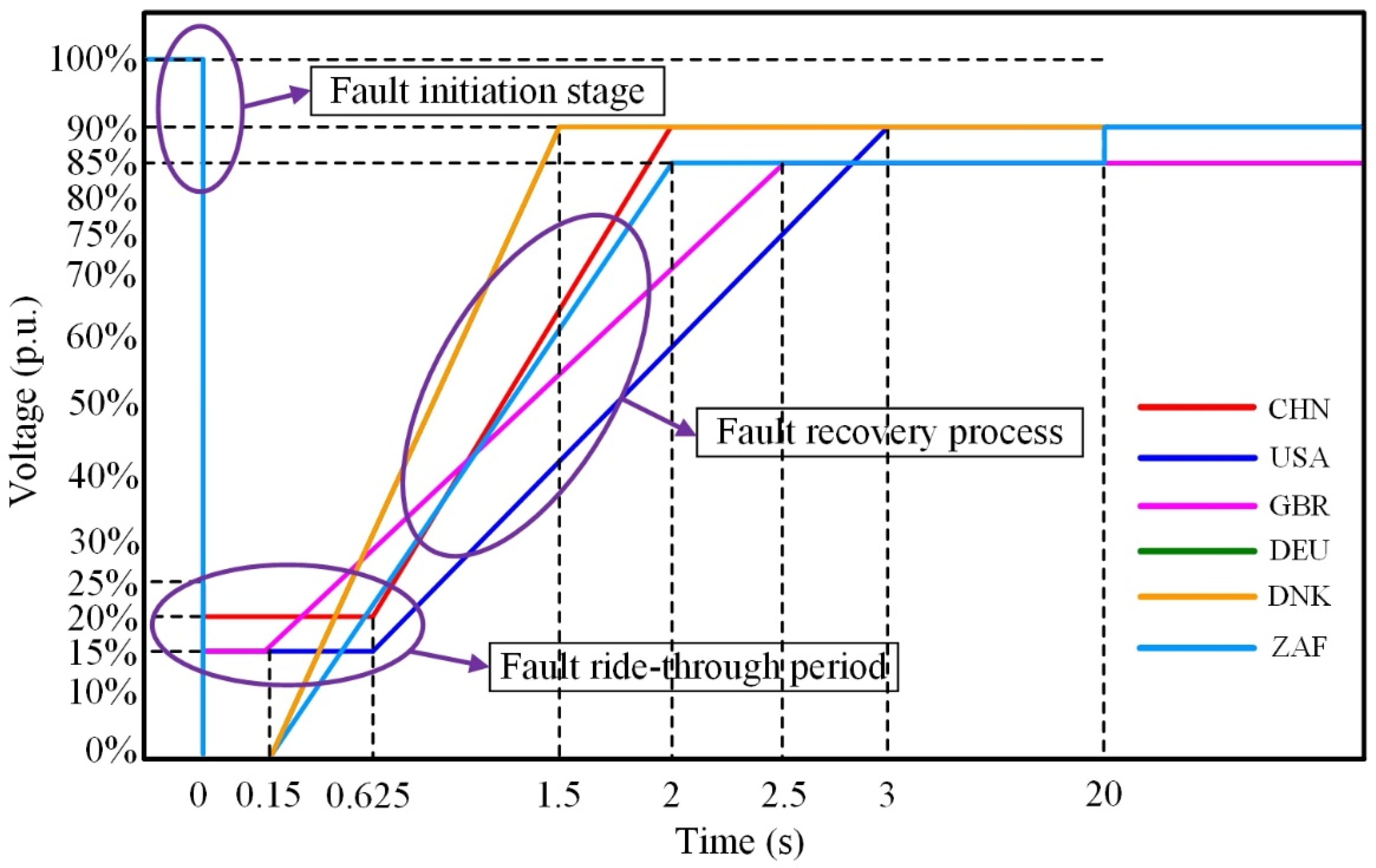
Part II: The common fault ride-through segmented control characteristics of new energy units are analyzed according to the high and low ride-through standards of new energy units in various countries, based on which a general structured model of three-segment control of wind turbine fault ride-through is established, and the core control parameters of the control strategies in each phase are analyzed.

Part III: The RTLAB hardware in-loop test simulation platform is utilized to conduct in-loop testing of the actual doubly fed wind turbine black box controller and to obtain the output response data of the controller under various operating states. Aiming at the measured data, a method of data segmentation preprocessing using the statistical modal feature segmentation method and a method for fast and accurate identification of structured models using the genetic Newtonian algorithm are proposed.

Part IV: According to the control identification method and various optimization algorithms proposed in this paper, a universal parameter identification software simulation platform is developed by combining Matlab App Designer and PSD-BPA.

Part V: The actual black box controller of a doubly fed wind turbine model that has been put into operation is selected for the RTLAB semi-physical hardware-in-the-loop test, and combined with the output response data, the parameter identification software platform, and the general structured electromechanical transient model of the doubly fed wind turbine, the parameter identification for the fault ride-through control of this doubly fed turbine’s black box controller is completed, and the simulation results of the different identification algorithms are compared in a variety of operating conditions. Which proves the validity and accuracy of the proposed parameter identification method and the developed software. The results demonstrate that the method proposed in this paper is more accurate and robust with higher engineering application value.

2. Characterization and Modeling of the Fault Ride-Through Process in Doubly Fed Wind Turbines

2.1. Characterization of the New Energy Unit Fault Ride-Through

The new energy grid connection standard serves as the basis for determining the control mechanism of new energy units. To summarize the typical characteristics of fault ride-through control among various new energy units, it is necessary to analyze and compare the new energy grid connection standards of different countries. Grid connection standards and FRT requirements for renewable energy units have been established internationally, with key regulations from China [39], the United States [40], the United Kingdom [41], Australia [42], Germany [43], Denmark [44], and South Africa [45], as comprehensively reviewed in [39,40,41,42,43,44,45]. The literature indicates that although the new energy grid connection standards of different countries vary in specific technical parameters, test conditions, and implementation details, the core principles and control objectives of FRT requirements exhibit significant commonalities. Common features:

① All standards require new energy units to maintain grid-connected operation for a certain length of time when the grid voltage drops to a certain level instead of going off-grid immediately and generally stipulate a deep drop tolerance of 0% to 20%.

② Most standards emphasize the need for the unit to provide a certain amount of dynamic reactive power support during a fault by outputting reactive current proportional to the voltage deviation in order to help the grid voltage recovery.

③ In order to avoid power impact after fault removal, countries generally limit the active recovery rate, requiring the unit active power to gradually restore output at a rate of 10~20% of rated power/second.

In addition, some new energy grids with high penetration rates also impose high voltage ride-through (HVRT) requirements to ensure that the units can continue to operate stably during voltage surges. These common features indicate that global new energy grid connection standards adhere to the core principle of “fault ride-through tolerance, dynamic support, and orderly recovery” in fault ride-through control. The differences are mainly reflected in the parameter setting and regional grid adaptability. In contrast, the convergence of control objectives lays the foundation for coordinating international standards and the generalized design of units. Figure 1 and Figure 2 show the comparison of new energy low voltage ride-through (LVRT) and high voltage ride-through (HVRT) standards in different countries, which demonstrates the similarities and differences in voltage tolerance range and duration in different countries;

Table 1. Comparison of LVRT technical parameters of new energy units in different countries.

Country/Standard	Voltage Dip Range	Reactive Current (Iq) Support Formula	FRT Duration	Recovery Process Requirements
CHN (GB)	0.2~0.9 UN	K × (0.9-Ut)	625 ms	Restore to 0.9 UN within 2 s
USA (FERC)	0.15~0.9 UN	K × (0.9-Ut)	625 ms	Restore to 0.9 UN within 3 s
GBR (NGC)	0.15~0.85 UN	K × (0.85-Ut)	140 ms	Restore to 0.85 UN within 2.5 s
DEU (EON)	0.0~0.9 UN	K × (0.9-Ut)	150 ms	Restore to 0.9 UN within 1.5 s
DNK (UCTE)	0.0~0.9 UN	K× (0.9-Ut)	150 ms	Restore to 0.9 UN within 1.5 s
ZAF (RSA)	0.0~0.85 UN	K × (0.85-Ut)	150 ms	Restore to 0.85 UN within 2 s, then to 0.9 UN within 20 s

and

Table 2. Comparison of HVRT technical parameters of new energy units in different countries.

Country/Standard	Voltage Swell Range	Reactive Current (Iq) Support Formula	Continuous Operation Time During Fault
CHN (GB)	1.1~1.3 Un	K × (Ut-1.1)	(1.1~1.2) Un: Remain connected for 10 s (1.2~1.25) Un: Remain connected for 1 s (1.25~1.3) Un: Remain connected for 0.5 s
USA (WECC)	1.1~1.2 Un	K × (Ut-1.1)	(1.1~1.15) Un: Remain connected for 3 s (1.15~1.175) Un: Remain connected for 2 s (1.175~1.2) Un: Remain connected for 1 s >1.2 pu: Tripping allowed
AUS (NER)	1.1~1.3 Un	K × (Ut-1.1)	(1.1~1.3) Un: Remain connected for 0.6 s Recover to 1.1 Un within 0.9 s
DEU (EON)	1.2~1.4 Un	K × (Ut-1.2)	(1.1~1.15) Un: Remain connected for 60 s (1.15~1.2) Un: Remain connected for 5 s >1.2 pu: Remain connected for 0.1 s
DNK (UCTE)	1.2~1.3 Un	K × (Ut-1.2)	(1.2~1.3) Un: Remain connected for 0.1 s
ZAF (RSA)	1.1~1.2 Un	K × (Ut-1.1)	(1.1~1.15) pu: Remain connected for 2 s (1.15~1.2) pu: Remain connected for 0.16 s

show the comparison of specific requirements of low and high voltage ride-through technical parameters in different countries, including reactive current support ratio, fault ride-through recovery time, and other key indicators.

As can be seen from the comparison of the waveforms of the new energy unit fault ride-through criteria in Figure 1 and Figure 2, the fault ride-through process of new energy units can be divided into three segments, which are the fault initial phase, the fault ride-through period, and the fault recovery process, in which the fault initial phase starts from the instant of grid fault occurrence and lasts for a short period (usually from a few milliseconds to tens of milliseconds); the fault ride-through period is the stage from the fault stabilization to the fault clearance, and the duration depends on the grid standard (e.g., the low voltage needs to be maintained from 150 ms to 1.5 s); and the fault recovery process is the transition stage from the fault clearing (voltage restoration) to the return of the unit to the normal operation state. It lasts from hundreds of milliseconds to several seconds. Although there is a high transient risk in the initial stage of the fault, the crowbar or chopper protection circuits of the converter can respond quickly in milliseconds, making the risk in this stage completely controllable and having a limited impact on the system. The latter two phases rely on active control strategies, which must match the dynamic characteristics of the grid and are directly related to the unit’s adaptability to the grid; therefore, their control performance is the most critical in the fault ride-through process. During the fault ride-through period, the short transient shock of the initial stage has been attenuated. The new energy unit switches to the fault ride-through control strategy, under which the new energy unit needs to maintain a specific non-off-grid continuous operation duration according to the depth of the fault voltage drop and outputs the corresponding reactive currents to support the recovery of the transient voltage; and in the stage of the fault recovery process, the unit has to be switched to the normal control mode again after the fault is cleared, and the external active current is output to the grid. During the fault recovery process, after the fault is cleared, the unit should immediately switch back to normal control mode. The external active and reactive power output should then be gradually restored to the expected value at a specific rate or according to a preset curve.

In summary, the fault ride-through process of new energy units presents typical staged dynamic characteristics, and its control modeling needs to adopt a multi-stage coupled modeling approach. By establishing the stage division criterion based on the fault characteristics, constructing the dynamic equations of each stage, and designing the smooth switching logic and parameter synergistic optimization, we can realize the accurate characterization of transient nonlinear characteristics, active support capability, and dynamic regulation characteristics of new energy units, which provides a theoretical foundation for improving the accuracy and generality of modeling of new energy units. It provides a theoretical basis for improving the accuracy and versatility of new energy unit modeling.

2.2. Structured Model of Electromechanical Transient of Doubly Fed Wind Turbine

Structured modeling refers to the method of independent packaging and modeling of the main internal functional modules according to the system structure, in which each functional module is designed as an independent and reusable structural block, which can be directly combined with the required structural blocks, thus forming a complete system simulation model efficiently and flexibly. The structure of the doubly fed wind turbine electromechanical transient model is shown in Figure 3, which is divided into the primary circuit and control circuit. Moreover, the primary circuit consists of the generator, converter, filter, and transformer, and the control part mainly includes the following:

(1) Mechanical side control and FM inertia control module;

(2) Outer-loop optimal speed tracking control, constant power control, constant DC voltage control, and inner-loop current control module during regular operation;

(3) A three-segment control module for the fault ride-through process when voltage disturbances occur in the grid.

The control system of the doubly fed wind turbine electromechanical transient structured model adopts the adaptive switching strategy based on the voltage state of the grid point, and its operation mechanism can be described as follows: the mechanical side control module firstly calculates the generator rotor torque T_gen and rotational speed ω_gen based on the input wind speed V_wind, and at the same time, the voltage monitoring unit detects the voltage U_t of the grid point in real-time and generates the binary control signal (0 means normal, 1 means fault) based on whether or not the voltage is out of the rated range. After that, the system switches to the corresponding control module based on the signal and generates active/reactive reference values P_ref, Q_ref, and dq-axis current commands I’_dref and I’_qref by integrally processing T_gen, ω_gen, U_t, and the voltage reference value U_ref. Finally, through the converter’s inner-loop current control and coordinate transformation, it outputs the equivalent controlled voltage source commands E_dp and E_qp, thus realizing the dynamic regulation of the unit’s output power and ensuring a fast power response capability during the power grid’s transient process. The structured mathematical model of the electromechanical transient of the doubly fed wind turbine in this paper is based on the standardized modeling methodology of the China Electric Power Research Institute (CEPRI), which can be found in the PSD-ST Transient Stabilization Program user manual [46].

2.2.1. Mechanical Side Control and FM Inertia Control Modules

• Mechanical side control module;

The mechanical side control module is the key component in completing the maximum wind energy tracking function. Its internal components usually consist of the wind turbine model, shaft system model, and pitch angle control model, all of which work together. The wind turbine model embodies the efficiency of converting wind energy into mechanical energy. The wind turbine model mathematical model is as follows:

$$\left\{\begin{array}{l}{P}_{\mathrm{m}}={\displaystyle \frac{1}{2}}\rho \pi C_{\mathrm{p}}\left(\lambda ,\beta \right){\mathrm{V}}_{wind}^3{R}^2\\ {\omega }_{\mathrm{m}}={\displaystyle \frac{{\nu }_{wind}}{R}}\\ T_{\mathrm{m}}={\displaystyle \frac{P_{\mathrm{m}}}{{\omega }_{\mathrm{m}}}}={\displaystyle \frac{1}{2}}\rho \pi C_{\mathrm{p}}\left(\lambda ,\beta \right){\nu }_{wind}^2{R}^3\\ C_p\left(\lambda ,\beta \right)=c_1\left({\displaystyle \frac{c_2}{{\lambda }_1}}-c_3\beta -c_4\right)e^{{\displaystyle \frac{-c_5}{{\lambda }_1}}}+c_6\lambda \\ {\displaystyle \frac{1}{{\lambda }_1}}={\displaystyle \frac{1}{\lambda +0.08\beta }}-{\displaystyle \frac{0.035}{{\beta }^3+1}}\end{array}\right.$$

(1)

where P_m is the output power of the prime mover (wind turbine), T_m is the output torque of the wind turbine, ρ is the air density, V_wind is the actual wind speed, R is the radius of the wind turbine impeller, ω_m is the angular velocity of the wind turbine machinery, C_p(λ,β) is the power coefficient of the wind turbine, λ is the optimal tip speed ratio of the wind turbine, and β is the pitch angle of the paddle. c₁–c₆ are, respectively, 0.5176, 116, 0.4, 5, 21, and 0.0068.

The shaft system model simulates the equations of motion of the drive shaft rotor, which mainly includes two parts, the low-speed shaft and the high-speed shaft, and is generally simulated by two mass-block models (the wind turbine and the generator as two mass-blocks), and ignores the damping coefficients of the wind turbine and the generator itself, so the complete two-mass-block dynamic mathematical model of the shaft system is as follows:

$$\left\{\begin{array}{l}2H_{\mathrm{W}}{\displaystyle \frac{d{\omega }_{\mathrm{m}}}{dt}}=T_{\mathrm{m}}-K_s{\theta }_{\mathrm{m}g}-D_s\left({\omega }_{\mathrm{m}}-{\omega }_{gen}\right)\\ 2H_{\mathrm{G}}{\displaystyle \frac{d{\omega }_{g\mathrm{en}}}{dt}}=T_{gen}+K_s{\theta }_{\mathrm{m}g}+D_s\left({\omega }_{\mathrm{m}}-{\omega }_{gen}\right)\\ {\displaystyle \frac{d{\theta }_{\mathrm{m}g}}{dt}}={\omega }_{base}\left({\omega }_{\mathrm{m}}-{\omega }_{gen}\right)\end{array}\right.$$

(2)

where H_W and H_G are the inertia time constants of the wind turbine and generator rotor, respectively; T_gen is the generator rotor torque; ω_gen is the generator rotor angular velocity; K_s is the stiffness coefficient of the shaft system; D_s is the damping coefficient between the wind turbine and the generator; θ_mg is the torsion angle of the wind turbine concerning the rotor of the generator; and ω_base is the rated rotational speed of the generator.

The pitch angle control model embodies the wind turbine’s control of the aerodynamic characteristics of the blades and the output power of the wind turbine, which can change the angle between the blade and the rotating plane according to the command value, thus achieving the effect of controlling the wind power absorbed by the wind turbine, and its control model is shown in Figure 4. It mainly plays two roles: when the wind speed is too large, the absorbed wind power is reduced by increasing the pitch angle; when the system encounters faults such as a three-phase short-circuit, in order to avoid rotor overload caused by the mechanical power being more significant than the electromagnetic power, the pitch angle also needs to be adjusted.

In Figure 4, ω_ref is the best reference value of generator speed under the actual wind speed; P_gen is the active power output from the generator; P_ref is the reference value of active power output from the operation state control module; T_r is the time constant of rotational speed measurement; T_pr is the time constant of electromagnetic power measurement; Kcc is the transfer coefficient; K_p, K_i are the coefficients of the rotational speed control proportional integral link; K_pp and K_pi are the electromagnetic power proportional integration link coefficients; β_max and β_min are the maximum and minimum limits of the pitch angle; and dβ_max and dβ_min are the maximum and minimum speeds of change of the pitch angle.

2.

FM Inertia Control Module;

The FM inertia control module is used to provide inertia characteristics similar to those of a conventional generator when simulating frequency changes. For example, when the frequency drops, the rapid control of power electronics and the inertia of the unit rotor are utilized to temporarily increase the unit’s active power output and reduce the frequency drop for a short period. Since the FM inertia control module is mostly an optional function in new energy units, and its influence on system identification or steady-state operation is negligible, it usually presents a closed state in the structured model control. The control model of the FM inertia control module is shown in Figure 5.

In Figure 5, f is the actual voltage frequency of the system grid point; f_ref is the reference value of the system frequency; Δf_{ab_pos} is the dead zone of the positive frequency deviation; Δf_{ab_neg} is the dead zone of the negative frequency deviation; Δf_max is the maximum value of the positive frequency deviation; Δf_min is the maximum value of the negative frequency deviation; dP/df_UP is the power change rate corresponding to positive frequency deviation; dP/df_DN is the power change rate corresponding to negative frequency deviation; df_max is the upper limit of the power change; df_min is the lower limit of the power change; dbwi is the inertia control positive frequency deviation dead zone; T_lpwi is the inertia control first-order inertia time constant; K_wi is the inertia control scaling coefficient; T_wowi is the inertia control differential time constant; P_mxwl is the upper limit of the inertia control power change; P_mnwl is the lower limit of the inertia control power change; urlwi is the upper limit of the inertia control power change rate; and drlwi is the inertia control power lower limit of the rate of change of inertia control power.

2.2.2. Normal Operation Active and Reactive Power Control Module

• Normal active and reactive power outer loop control module;

The control block diagram of the normal operation active and reactive power control module of the structured model of the new energy unit proposed in this paper is shown in Figure 6, in which the outer-loop active power control strategy includes outer-loop control of wind turbine speed, constant power factor control, and constant DC voltage control. The outer-loop normal operation control utilizes the output variables of the mechanical side control to generate reference values for active and reactive power, thereby controlling the inner loop and achieving complete double closed-loop control. Additionally, part of the outer loop control can also directly generate the initial active and reactive current reference values in some instances, further improving the response speed of the controller.

In Figure 6a, T_pε is the rotational speed time constant; K_pvq is the proportional coefficient of the rotational speed control link; K_ivq is the integral coefficient of the rotational speed control link; T_pc is the power time constant; (dP/dt)max is the maximum rate of change of the power; (dP/dt)min is the minimum rate of change of the power; T1 is the time constant of DC voltage measurement; K_pudc is the proportional coefficient of the DC voltage control link; K_iudc is the DC voltage control link proportionality coefficient; In Figure 6b, Z_c is the voltage compensation impedance; T_r is the time constant of grid-connected voltage measurement; K_pu is the proportionality coefficient of constant voltage control; K_iu is the integral coefficient of constant voltage control; T_u is the time constant of reactive power measurement; Q_max is the maximal value of reactive power; Q_min is the minimal value of reactive power; T_PE is the time constant of active measurement; PF_ref is the constant power factor angle.

2.

Inner loop current control module;

The converter inner-loop current control module adopts multi-strategy independent control architecture for active and reactive power. The inverter inner-loop active current control mode includes active power direct voltage removal and active power PI control; the inverter inner-loop reactive current control mode includes reactive power direct voltage removal, reactive power PI control, and reactive power and voltage coordinated control. As shown in Figure 7, in the inner-loop current control structure, the system collects the output P_gen and Q_gen in real-time and carries out the PI closed-loop control operation with the reference values of P_ref and Q_ref from the output of the outer-loop control and ultimately generates the initial active current reference value I’_dref and the reactive current reference value I’_qref. The control modes can be switched seamlessly according to the grid operation demand. Each control mode can be switched according to the grid operation requirements, where the PI control adopts an anti-saturation integral algorithm to ensure current limiting protection during the dynamic response process.

In Figure 7, Ut is the real-time voltage at the parallel network point; I_dmax and I_dmin are the maximum and minimum values of active current; I_qmax and I_qmin are the maximum and minimum values of reactive current; U_max and U_min are the maximum and minimum values of output voltage; K_pp and K_pi are the integral coefficients of the active control ratio; K_qp and K_qi are the integral coefficients of the reactive control ratio; and K_up and K_ui are the integral coefficients of the voltage control ratio.

2.2.3. Fault Ride-Through Operation Active and Reactive Power Control Module

In this paper, the fault ride-through active and reactive power control module adopts a three-segment control simulation method, as shown in Figure 8. The active and reactive power control of the model during the whole fault process is decomposed into three-segment control phases during the fault ride-through period (①), the starting point of the fault recovery (②), and the fault recovery process (③), and each of these control phases contains a variety of different control strategies. As shown in Figure 9, the control of the unit before and after the fault can be achieved by modifying the control strategy and key control parameters of each control phase for active or reactive power after determining the power priority.

• Control modeling during fault ride-through;

The active control methods commonly used during fault ride-through of structured models include specified active power, specified active current, and low-voltage-limited active current control. The reactive control methods are specified reactive power and specified reactive current. The mathematical expression for the active control methods during fault ride-through is as follows:

$$\left\{\begin{array}{l}{P}_{\mathrm{ref}}=K_p\times P_0+P_{\mathrm{set}}\\ I_{d\mathrm{ref}}^{\prime }=K_{\mathrm{vp}}\times U_t+K_{\mathrm{Id}}\times I_{d0}+I_{d\mathrm{set}}\\ I_{d\mathrm{ref}}^{\prime }=I_{d0}\\ I_{d\mathrm{ref}}^{\prime }={\displaystyle \frac{I_{\mathrm{L}\mathrm{V}\mathrm{R}\mathrm{T}\_\mathrm{U}\mathrm{P}}}{U_{\mathrm{UP}}-U_{\mathrm{down}}}}\times (U_t-U_{\mathrm{down}})\end{array}\right.$$

(3)

where K_p is the active power coefficient, P₀ is the initial active power; P_set is the active power control value during fault ride-through; K_VP, K_Id are the active current coefficients; I_d0 is the initial active current; I_dset is the active current control value during the ride-through period; I_{LVRT_UP} is the upper current threshold value; U_UP is the upper voltage threshold value; and U_down is the lower voltage threshold value.

The mathematical expression for the reactive power control mode during fault ride-through is as follows:

$$\left\{\begin{array}{l}{Q}_{\mathrm{ref}}=K_q\cdot Q_0+Q_{\mathrm{set}}\\ I_{q\mathrm{ref}}^{\prime }=K_{vq}\cdot \left(U_{\mathrm{set}}-U_{\mathrm{t}}\right)+K_{Iq}\cdot I_{q0}+I_{q\mathrm{set}}\end{array}\right.$$

(4)

where K_q is the reactive power coefficient; Q₀ is the initial reactive power; Q_set is the reactive power control value during the ride-through; K_vq and K_Iq are the reactive current coefficients; U_set is the fault ride-through voltage threshold; I_q0 is the initial reactive current; I_qset is the reactive current control value during the ride-through.

2.

Fault Recovery Starting Control Model;

The active control modes for fault recovery starting point control are specified as active current, active current during a fault, and active power during a fault; the reactive control modes are specified as reactive current, initial reactive current, and reactive power during a fault. The mathematical expression for the active control mode of fault recovery starting point control is as follows:

$$\left\{\begin{array}{l}{I}_{d\mathrm{ref}}^{\prime }=\min (K_{Id\_\mathrm{start}}\cdot I_{d0}+I_{d\mathrm{set}\_\mathrm{start}},I_{d0})\\ I_{d\mathrm{ref}}^{\prime }=I_{dFRT}\\ P_{\mathrm{ref}}=P_{FRT}\end{array}\right.$$

(5)

where K_{Id_start} is the active current coefficient of recovery starting point; I_{dset_start} is the active current control of recovery starting point; I_dFRT is the active current during fault ride-through; and P_FRT is the active power during fault ride-through;

The mathematical expression for the reactive power control method for fault recovery starting point control is as follows:

$$\left\{\begin{array}{l}{I}_{q\mathrm{ref}}^{\prime }=K_{Iq\_\mathrm{start}}\cdot I_{q0}+I_{q\mathrm{set}\_\mathrm{start}}\\ I_{q\mathrm{ref}}^{\prime }=I_{q0}\\ Q_{\mathrm{ref}}=Q_{FRT}\end{array}\right.$$

(6)

where K_{Iq_start} is the recovery starting point reactive current factor; I_{qset_start} is the recovery starting point reactive current control; and Q_FRT is the active power during fault ride-through;

3.

Fault Recovery Process Control Model;

The active control modes of fault recovery process control are immediate recovery without control, specified slope recovery, and recovery by inertia curve; the reactive control modes are immediate recovery without control and recovery control by inertia curve. The mathematical expression of the active control mode of fault recovery process control is as follows:

$$\left\{\begin{array}{l}{P}_{\mathrm{ref}}=K_{\mathrm{slope}}\cdot t+P_{\mathrm{icept}}\\ P_{\mathrm{ref}}=P_{T_3}+(1-{\mathrm{e}}^{\left(-{\displaystyle \frac{t-T_3}{T_P}}\right)})\end{array}\right.$$

(7)

where K_slope is the active recovery slope of the fault process; t is the recovery time; P_icept is the longitudinal intercept value of the active power of the recovery process; P_T3 is the initial value of the active power of the fault recovery process; T_p is the active inertia recovery time constant of the fault recovery process, and T₃ is the start time of the fault recovery process.

The mathematical expression for the reactive power control method for fault recovery process control is as follows:

$$Q_{\mathrm{ref}}=Q_{{\mathrm{T}}_3}+({\mathrm{e}}^{\left(-{\displaystyle \frac{t-T_3}{T_q}}\right)}-1)$$

(8)

where Q_T3 is the initial value of reactive power for the recovery process, and T_q is the reactive inertia recovery time constant for the fault recovery process.

2.3. Analysis of Core Control Parameters for Fault Transient Processes

In the parameter identification study of the structured model of a new energy unit, the reasonable selection of the identification parameter set is the key to ensuring the model’s accuracy and identification efficiency. About the topological characteristics and dynamic response mechanism of the structured model of the new energy unit in this paper, the parameter identification needs of non-critical control modules can be systematically excluded. On the one hand, the time constants of the mechanical side control and FM inertia control modules are generally more significant than the millisecond dynamic process of the fault ride-through process, and their parameters have lower coupling to the transient characteristics; on the other hand, the active/reactive control module under normal operating conditions will be forced to block during faults, and its parameter impact on the fault response characteristics is negligible. The PI parameters of the inverter inner-loop current control module adopt the voltage feedforward decoupling strategy so that its PI parameters have negligible influence on the fault response characteristics. In addition, although the mechanical side control module can characterize the mechanical dynamics of the wind turbine, its second-time scale is significantly decoupled from the millisecond transient process of grid faults, so it is also not required to be included in the identification system.

From the analysis of the structured model fault ride-through control in the previous section, it can be seen that the fault ride-through active and reactive power control module, as the core control link of the model in the case of grid fault perturbation, the three-segment control strategy of the fault ride-through and its key control parameters directly determine the dynamic response characteristics of the unit. Hence, determining the fault ride-through control strategy and the control parameters to be identified is the basis for guaranteeing the accuracy of the identification simulation results. Therefore, determining the control strategy and control parameters to be recognized in the fault ride-through control process is the basis for guaranteeing the accuracy of the identification simulation results, and the control parameters of the whole fault ride-through process are shown in

Table 3. Fault transient process core control parameters.

Fault Transient Segmentation	Active Power Control Parameters	Reactive Power Control Parameters
During fault ride-through	Kp, Pset, Kvp, Kid, Idset, ILVRT_UP, UUP, Udown	Kq, Qset Kvq, Kiq, Iqset,
Fault recovery starting	Kid_start, Idset_start	Kiq_start, Iqset_start,
Fault recovery process	Kslope, Tp	Tq

:

The initial active power and active current and the initial reactive power and reactive current in the structured model are the input reference values during normal control operation; therefore, analyzing the mathematical expressions of the fault ride-through three-segment control, it can be seen that the initial parameters P₀, Q₀, I_d0, and I_q0 have no influence on the power and current changes during the fault period. In addition, the structured model fault ride-through conditions can be divided into four typical scenarios: symmetrical low/high fault ride-through and asymmetrical low/high fault ride-through. In order to comprehensively validate the applicability of the model and the fault ride-through control identification to different types of fault conditions, it is necessary to analyze the ride-through characteristics of different types of faults in a differentiated manner and to identify the fault ride-through three-segment control strategy and the control parameters of the faults under the various types of faults, respectively.

3. Parameter Identification of Black Box New Energy Units

3.1. A Black Box New Energy Unit Fault Ride-Through Control Parameter Identification Method Based on Measured Data

In order to identify the parameters of the new energy structured model more efficiently and accurately, this paper adopts the proposed black box new energy unit structured model fault ride-through identification method based on measured data, and the specific flow is shown in Figure 10:

(1) Build a new energy controller semi-physical hardware-in-the-loop test simulation platform based on RTLAB and test the measured response data of the new energy actual controller under a variety of working conditions on this platform.

(2) Clean and preprocess the collected measured recorded waveform data of new energy under normal and fault conditions, including removing outliers, filling in missing values, and normalizing data amplitude. Then, valuable features are extracted from the preprocessed data to help the computer quickly and accurately identify the normal operation state and fault ride-through three-segment operation states of the data. After that, the measured operating condition data are divided into four sets: low penetration symmetric fault set, low penetration asymmetric fault set, high penetration symmetric fault set, and high penetration asymmetric fault set, based on the fault type. A corresponding fault classification model is then established for each set. Finally, each type of fault data set is divided into a training set and a test set according to the data usage.

(3) The measured response data set of a single fault type is selected. The statistical modal feature segmentation method is utilized to segment the fault ride-through into three segments (fault ride-through period, fault recovery starting point, and fault recovery process) of the training set and test set condition data under the jurisdiction of the training set to obtain the segmented data of the training set and the segmented data of the test set.

(4) Aggregate the fault ride-through three-segment data of the training set conditions, and use the genetic Newton algorithm cycle to optimize the key control parameters of the multi-strategy control model of the fault ride-through three-segment control, calculate the size of the adaptive value of each individual in the population according to the objective function (Equation (1)) after each iteration and rank them, select the optimal parent individual according to the principle of the smaller, the better the adaptive degree, and carry out the cross-mutations to generate a new generation of populations. The cycle repeats until the adaptation degree of iterative individuals meets the threshold requirement or reaches the maximum number of iterations and then jumps out of the genetic optimization, after which, according to the suitable solution region searched by the genetic algorithm, the limited-memory Broyden–Fletcher–Goldfarb–Shanno (L-BFGS) algorithm is used to carry out the refinement of parameter optimization. By comparing the size of the final adaptation value of each control strategy under the same control stage, the optimal combination of control strategies and their control parameters are quickly outputted, and finally, the structured simulation model of the electromechanical transient state of the black box new energy unit is constructed by synthesizing the basic information of the actual capital collection and the optimal identification results.

$$J(k)=\sqrt{{\displaystyle \frac{1}{\mathrm{n}}}{\displaystyle \sum _{\mathrm{i}=1}^{\mathrm{n}}{\left(y_{\mathrm{real}}\left(\mathrm{i}\right)-y_{\mathrm{sim}}\left(\mathrm{i}\right)\right)}^2}}$$

(9)

where y_real and y_sim are measured data values and model fitting outputs, respectively.

(5) Select the test set segmentation data with the same fault type for the verification of identification results, extract the power size, fault type, fault start and end time, and other fault characteristic parameters of the test set of measured conditions, and import the fault characteristic parameters of the test set of conditions into the structured simulation model of the new energy unit of the black box in a cycle for simulation to ensure that the measured model and the structured model in the fault ride-through condition simulation have the same depth and duration of the voltage dips. After the simulation is completed, all the simulation data of the structured model under the fault type are exported, and the deviation between the simulation and the measured data is calculated according to the Chinese national standard GB/T44650-2024 [47]. If the deviation of all the conditions meets the standard requirements, the optimal identification results can be considered as the equivalent control of the black box new energy unit under this fault type; if there are test conditions whose deviation does not meet the requirements, it is necessary to carry out the test again after re-identification or modification of the original identification results until the error results of all the test sets of conditions meet the standard requirements.

(6) After completing the identification and examination of the optimal control of the structured model of the black box new energy unit under four types of faults according to the above method, a structured simulation model that can fully characterize the fault ride-through characteristics of the actual black box unit is finally obtained. The resulting structured model of the new energy unit is simulated for both high and low-fault ride-through scenarios, and the corresponding reactive power support coefficients and active recovery coefficients are calculated and compared with the values stipulated in the national standard to evaluate the fault ride-through performance of the structured model of the black box unit.

3.2. Semi-Physical Hardware-in-the-Loop Test of RTLAB-Based Black Box New Energy Unit Controller

The black box new energy unit RTLAB hardware-in-the-loop simulation test is a method that utilizes the real-time digital simulator RTLAB and the actual controller of the new energy unit to construct a closed-loop test environment and conduct a series of fault ride-through tests. This method is the most common in the testing of large-capacity power electronic devices, which not only can reflect the dynamic response characteristics of the device comprehensively, adequately, accurately, and efficiently but also has a lower cost, a higher automation rate, and a higher safety factor compared with the purely physical test method.

The semi-physical hardware-in-the-loop test platform of the black box new energy unit controller based on RTLAB is shown in Figure 11. The RTLAB simulation platform and the black box controller interact with each other through the bi-directional DB37 line for the control signals and electrical quantities. The host computer controls and monitors the operating commands and signals of the RTLAB simulation platform and the controller through a bi-directional high-speed fiber optic or network cable. Before carrying out the test, it is necessary to build the primary circuit model and user signal observation interface of the corresponding new energy unit in the real-time digital simulation software RT-LAB installed in the host computer. Considering the high switching frequency of the new energy inverter, it is generally chosen to be built in a small-step environment. After the virtual model is constructed, the generated C code is downloaded to the RTLAB simulation platform using the compilation and download function of the software.

During the test operation, the RTLAB simulation platform and the black box controller carry out real-time bidirectional signal communication through the GTAO\GTDI analog-to-digital converter board and I/O interface. After receiving the voltage and current feedback signals from the RTLAB virtual model, the actual controller calculates the corresponding PWM control signals according to its operation state and, at the same time, transmits the PWM control signals to the RTLAB simulation platform, which then uses the PWM signals to complete the control of the virtual model inverter, thus finally forming a closed-loop simulation of the whole grid-connected system. RTLAB simulation platform: The RTLAB platform then uses the PWM signals to complete the control of the virtual model inverter, thus finally forming a closed-loop simulation of the entire unit grid-connected system.

In the whole closed-loop simulation process, the grid-connection commands of the RTLAB virtual model, fault settings, parameter changes of the unit, as well as the changes of the actual controller control parameters and power regulation parameters are all accomplished through the RTLAB user interface control module of the host computer. In contrast, all the operation data of the simulation system and the operation status signals of the controllers are uniformly received and observed through the RTLAB user interface data receiving and observing module.

As shown in Figure 12a,b, in order to verify the effectiveness of the proposed structured model fault ride-through control identification method, this paper takes a wind power black box unit as an example. The semi-physical test system for grid-connected doubly fed wind turbines is built within the RTLAB real-time simulation platform. The output response of the new energy black box controller is tested in-loop in a variety of working conditions according to the Chinese national standard GB/T44650-2024 parameter test protocol document. The output response of the controller is tested in the loop. The measured response data of the controller is also obtained by using recorded waveforms, in which the recorded variables include the instantaneous values of the three-phase voltages and currents at the measurement point, the fundamental positive sequence component U_sim of the output voltage, the active power P_sim, the reactive power Q_sim, the active current I_dsim, and the reactive current I_qsim.

3.3. Processing of Measured Data and Selection of Optimization Algorithms

3.3.1. Data Segmentation Preprocessing Based on Statistical Modal Features

When carrying out the identification of active and reactive three-segment control models for each fault type, the selection of a precise segmentation of the training set data and a reliable optimization algorithm will determine the accuracy of the identification results. Therefore, this paper firstly analyzes the statistical characteristics of the measured data and proposes a segmentation method based on the statistical modal characteristics, which utilizes the centralized trend characteristics of voltage, active, and reactive data during fault ride-through and recovery to segment the data and divides the whole data segment into six parts shown in Figure 13. The specific segmentation steps are shown below:

(1) Based on the received controller fault ride-through voltage thresholds and voltage data, initially determine the starting point Sin for entering the fault ride-through state and the termination point Sout for exiting the fault ride-through state for the working condition in which it is located.

(2) Extract the statistical modal eigenvalues of voltage, active power, and reactive power during the fault ride-through phase, i.e., the steady-state values during the fault ride-through period, using the initial starting and ending data point locations.

(3) Setting the deviation threshold and combining with Equation (2), first determine the data start and end points of voltage, active power, and reactive power during the fault ride-through period, and then take a large for the data start point of each variable to obtain the start point S1 of the fault ride-through period, and take a small for the data endpoint of each variable to obtain the endpoint S2 of the fault ride-through period.

$$\begin{array}{l}S{1}_{\mathrm{var}}=\min \{i|{\displaystyle \frac{dat{a}_{\mathrm{var}}(i)-mod{e}_{\mathrm{var}}}{mod{e}_{\mathrm{var}}}}\mid <DEV\}\\ S{2}_{\mathrm{var}}=\max \{i|{\displaystyle \frac{dat{a}_{\mathrm{var}}(i)-mod{e}_{\mathrm{var}}}{mod{e}_{\mathrm{var}}}}\mid <DEV\}\end{array}$$

(10)

where S1_var and S2_var are the start and end point positions during fault ride-through for each variable; data_var is the fault ride-through data for each variable; mode_var is the steady-state value during fault ride-through for each variable; and DEV is the deviation threshold.

(4) Similarly, the data of each variable starts from the endpoint S2 of the fault ride-through period, firstly extracts the normal steady-state value of each variable, and then combines with Equation (2) to obtain the starting point position of each variable to enter into the normal steady-state operation after the fault, i.e., the position of the endpoint of each variable’s fault recovery process, and then takes the larger one to obtain the data’s endpoint S4 of the fault recovery process.

(5) For the fault recovery starting point phase, the starting point is the endpoint S2 of the fault ride-through period, and the endpoint S3 generally defaults to be the 10% to 20% position of the period from the endpoint S2 of the fault ride-through period to the endpoint S4 of the fault recovery process;

3.3.2. Genetic Proposed Newton Hybrid Optimization Algorithm

After completing the segmentation and categorization of all working condition data in the training set, combined with the proposed structured three-segment control model for active and reactive fault ride-through, the active and reactive multi-control strategy models contained in each stage are identified with their respective parameters. The control strategy with the smallest identification error is selected as the optimal control strategy for testing at that stage.

Due to the existence of both linear and nonlinear models in the control model to be identified and the large size and complexity of the measured sample set data of the model, if only a linear optimization algorithm is used, it is impossible to optimize the nonlinear model effectively. If only a nonlinear algorithm is used, it is easy for the optimization process to fall into a local optimum and fail to find the global optimal solution, which affects the quality of the optimization results and the accuracy of the model. To overcome the aforementioned problems, this paper employs a hybrid optimization approach combining a genetic algorithm with L-BFGS for parameter identification.

Genetic algorithm (GA) is a computational model simulating Darwinian natural selection, featuring strong global search capability that enables rapid approximation of optimal solutions in early stages. However, its local search ability tends to weaken in later stages. On the other hand, the limited-memory Broyden–Fletcher–Goldfarb–Shanno (L-BFGS) algorithm, as a quasi-Newton method, demonstrates excellent local convergence properties but is sensitive to initial values. Recognizing these complementary characteristics, this study develops a novel hybrid approach that organically combines both algorithms into a genetic quasi-Newton method [48]. The hybrid approach leverages the complementary strengths of both algorithms: the genetic algorithm’s strong global search capability and rapid initial exploration, combined with the Newton method’s (L-BFGS) fast local convergence. This integration addresses key limitations of each method—the genetic algorithm’s weakening local search ability in later stages and the Newton method’s sensitivity to initial values. The implementation involves two key components: (1) the genetic algorithm performs initial global exploration to identify promising solution regions, and (2) automatic switching to L-BFGS when population diversity falls below a threshold or fitness improvement stagnates. This synergistic combination effectively solves problems of slow optimization while preserving each algorithm’s strengths. The specific implementation method is as follows:

(1) Initialize the parameters related to the genetic Newtonian algorithm, including the population size M, the maximum number of iterations G_max, and the fitness threshold. Randomly generate the initial population P = {k₁,k₂,…, k_M}, and the population individual k_i is a parameter vector, where the jth parameter takes the value range of [k_{min_j},k_{max_j}].

(2) Calculate the fitness f(k_i) of each individual in the initial population using the objective function and rank them according to their size, and the fitness calculation formula is as follows:

$$f(k_i)={\displaystyle \frac{1}{J(k_i)+\epsilon }}$$

(11)

where ε is the anti-zero division positive number.

(3) Perform a selection crossover mutation operation according to the principle that the larger the fitness value, the better; use roulette to select the two parent individuals with higher fitness for a single-point crossover operation, and carry out a mutation operation on the generated offspring individuals to increase the diversity of the population to avoid the population from falling into the local optimal solution.

(4) Calculate the fitness value of the new individual; if it meets the fitness threshold or the maximum number of iterations, then exit the genetic optimization; if it does not meet, use the elite retention strategy to update the population again and recycle steps (2) and (3) until the fitness of the new individual or the number of iterations meets the requirements.

(5) The approximate solution obtained by the genetic algorithm serves as the initial solution for the proposed Newton method, which is then locally optimized to refine the solution’s accuracy. Calculate the gradient of the objective function J(k_best) of the current approximate solution k_best and update the approximation matrix of the Hessian (i.e., the approximation of the second-order derivatives), where the initial Hessian matrix H₁ is usually a unitary matrix, and the gradient is calculated with the following formula for updating the Hessian matrix:

$$\left\{\begin{array}{l}\mathsf{\nabla }J(k_{best})=-{\displaystyle \frac{1}{n\cdot J(k_{best})}}{\displaystyle \sum _n^{i=1}}\left(y_{\mathrm{real}}(i)-y_{\mathrm{sim}}(i,k_{best})\right)\cdot {\displaystyle \frac{d{y}_{\mathrm{sim}}(i,k_{best})}{d{k}_{best}}}\\ H_{k+1}=H_k+{\displaystyle \frac{y_k{y}_k^T}{y_k^T{s}_k}}-{\displaystyle \frac{H_k{s}_k{s}_k^T{H}_k}{s_k^T{H}_k{s}_k}}\\ y_k=\mathsf{\nabla }J(k_{k+1})-\mathsf{\nabla }J(k_k)\\ s_k=k_{k+1}-k_k\end{array}\right.$$

(12)

where S_k is the change in the current parameter update; y_k is the change in the gradient.

(6) The current parameters are re-updated based on the computed approximate solution k_best gradient, combined with the Hessian’s approximation matrix, updated by the following equation:

$$k_{\mathrm{new}}=k_{\mathrm{best}}-H_k^{-1}\mathsf{\nabla }J(k_{\mathrm{best}})$$

(13)

where $H_k^{-1}$ is the inverse of the Hessian matrix. k_new is the new approximate solution obtained by updating.

(7) Cyclically call steps (5) and (6) until the objective function value J(k) of the latest approximate solution converges to a sufficiently small threshold ϵ or the number of iterations reaches the upper limit, terminate the iteration of the proposed Newton method, and output the optimal solution.

3.4. Comparison Error Calculation

The calculation of transient steady-state deviation in the three segments of the fault ride-through control is shown in the Chinese national standard GB/T44650-2024, whose main purpose is to test the accuracy of the model by calculating the deviation between the simulation data of the structured model and the measured data. After completing the segmentation of simulation data and measured data for the test condition, the deviations of the electrical quantities in the normal steady state before fault occurrence, the transient steady state during fault ride-through, and the transient steady state after fault recovery are calculated, and the electrical quantities for which the deviations are to be calculated include the output voltage U, the active power P, the reactive power Q, the active current I_d, and the reactive current I_q. The types of deviations to be calculated include the average deviation in the transient interval of each period, the average deviation and maximum deviation in the steady-state interval, and the weighted average total deviation of the whole process. The formulas for calculating the average deviation, maximum deviation, and weighted average total deviation are as follows:

The average deviation FME of the steady state and transient intervals for each time period:

$$F_{\mathrm{ME}}={\displaystyle \frac{1}{\mathrm{N}}}\left|{\displaystyle \sum _{i=1}^N\left[X_{\mathrm{S}}(i)-X_{\mathrm{M}}(i)\right]}\right|$$

(14)

where X_S is the hardware-in-the-loop simulation data standardized value in the test interval; X_M is the model simulation data standardized value in the test interval; and N is the number of data in the test interval.

The average absolute deviation FMAE of the steady state and transient intervals for each time period:

$$F_{\mathrm{MAE}}={\displaystyle \frac{1}{\mathrm{N}}}{\displaystyle \sum _{i=1}^N\left|X_{\mathrm{S}}(i)-X_{\mathrm{M}}(i)\right|}$$

(15)

Maximum deviation from the steady-state interval FMXE:

$$F_{\mathrm{MXE}}=\underset{i=1\cdots N}{\max }\left[\left|X_{\mathrm{S}}(i)-X_{\mathrm{M}}(i)\right|\right]$$

(16)

Full process weighted average absolute deviation FG:

$$F_{\mathrm{G}}=10\%F_{\mathrm{MAE}1}+60\%F_{\mathrm{MAE}2}+30\%F_{\mathrm{MAE}3}$$

(17)

where F_MAE1 is the average deviation from the normal steady state before the fault; F_MAE2 is the average deviation from the transient steady state during fault ride-through; and F_MAE3 is the average deviation from the transient steady state for fault recovery.

The deviation calculation results between the simulation data and measured data of the new energy structured model for the test condition shall meet the following conditions: (1) The deviation of each voltage on the high-voltage side of the step-up transformer of the power generation unit of the new energy structured model for all the test conditions shall be no greater than the maximum permissible value of the voltage deviation in Table 2; (2) The average deviation of the current, the reactive current, the active power, and the reactive power in the steady state and the transient intervals for all the test conditions, the maximum deviation in the steady-state interval, and the weighted average total deviation should not be greater than the maximum permissible deviation in Table 2: (3) For the model simulation test under the two-phase asymmetrical fault condition, the maximum permissible deviation of the positive sequence component of the fundamental wave is 1.5 times the value in

Table 4. Maximum permissible deviation of the specified test quantity.

Electrical Parameters	FME_SS	FME_TS	FMXE_SS	FG
Positive sequence voltage	0.02	0.05	0.05	0.05
Active power	0.05	0.1	0.08	0.08
Reactive power	0.05	0.1	0.08	0.08
Active Current	0.05	0.1	0.08	0.08
Reactive Current	0.05	0.1	0.08	0.08

. Table 4 contains the national standard provisions for the detection of the maximum permissible deviation value of the electrical quantity.

In the table, F_{ME_SS} is the average deviation allowance for steady-state intervals; F_{ME_TS} is the average deviation allowance for transient intervals; F_{MXE_SS} is the maximum deviation allowance for steady-state intervals; and F_G is the weighted average absolute deviation allowance for all intervals.

4. Development of a New Energy-Structured Model Fault Ride-Through Identification Software Platform Based on Matlab and BPA

MATLAB App Designer, developed by Math Works, is an integrated development environment designed for rapidly building interactive applications that combine a graphical user interface (GUI) with object-oriented programming. Its key advantage is an intuitive and easy-to-use interface that allows researchers to create and deploy applications quickly with simple drag-and-drop operations. Leveraging MATLAB’s powerful computational and optimization libraries, App Designer excels in parameter identification, optimization, and data manipulation, enabling real-time parameter tuning and visualization of results. However, when dealing with complex power system simulation, especially new energy-structured modeling, the built-in functions of MATLAB App Designer may not be able to meet the demand for high-precision simulation and system dynamic behaviors, especially in the accurate simulation of new energy devices such as wind power and photovoltaic power plants after they are connected to the power grid. Therefore, it is often necessary to use it in combination with a dedicated simulation tool to ensure modeling accuracy.

PSD-BPA (Power System Dynamics-Bonneville Power Administration) is a comprehensive power system simulation tool developed by the China Electric Power Research Institute (CEPRI), widely used in tasks such as tidal current calculation and transient stability analysis, and excels particularly in modeling and dynamic simulation of wind power and photovoltaic systems. Although BPA has advantages in the stability analysis of new energy systems connected to the grid, its lack of flexible custom programming and algorithm design functions limits the realization of personalized analysis needs. In addition, the operation of BPA is more specialized, and ordinary users face a higher threshold of using it.

Based on this, this study combines the advantages of MATLAB App Designer and PSD-BPA to develop efficient parameter identification software for new energy-structured models. With the graphical interface provided by App Designer, researchers can easily adjust the parameters, view the identification results in real-time, and dynamically present the effects of parameter changes on the simulation results, which greatly simplifies the operation process. At the same time, with the powerful algorithm library of MATLAB, the software can efficiently identify and optimize the parameters and improve the identification accuracy and speed. Through the simulation function of PSD-BPA, it can accurately simulate the dynamic characteristics of the new energy equipment after connecting to the power grid and verify the accuracy and reliability of the parameters. This integrated solution makes up for the shortcomings of the MATLAB App Designer in simulation function and, at the same time, enhances the flexibility of the PSD-BPA in personalized identification and real-time optimization, which provides strong support for the control identification, parameter optimization, and engineering applications of new energy systems.

The main components of the parameter identification simulation software based on the joint development of MATLAB and PSD-BPA proposed in this paper include the data import and processing module, control parameter identification module, PSD-BPA program simulation inspection module, error calculation, and model evaluation module. The MATLAB main program consists of data processing, a parameter identification algorithm, and a BPA calling program. The specific working principle of the joint parameter identification software and the physical diagram of the software are shown in Figure 14 and Figure 15.

The main functions of each functional module of the software are as follows:

① Data Import and Processing Module: It is used to import measured data, classify them based on fault type and usage after step transformation, and segment all kinds of data according to the three segments of the fault ride-through and extract the characteristic parameters of faults in each working condition.

② Control Parameter Identification Module: Select the relevant optimization algorithm, set the initialization parameters, combine the optimization algorithm and the measured segmentation data to carry out a variety of control model parameter identifications, and determine the optimal control combination according to the results of the identification error of each model.

③ PSD-BPA Program Simulation and Inspection Module: Based on the optimal control combination obtained from the identification, the basic income information, and the characteristic parameters of working conditions and faults, construct the DAT power trend calculation model and SWI power stability calculation model corresponding to the electromechanical transient structural model of the new energy unit, and then call the power trend calculation program PFNT.EXE to calculate the DAT power trend model in parallel and obtain the result of the power trend. Then, combined with the power current result data and the power stability calculation program SWNT.EXE, the power SWI stability model is calculated in parallel to obtain the SWX simulation data files of the BPA unit structured model under various working conditions. The code of the BPA software calculation program is shown in Figure 16.

④ Error Calculation and Model Evaluation Module: It is used to calculate the error between the measured data and the .SWX simulation data under the same working condition, judge the advantages and disadvantages of the identification results according to the error results, evaluate the fault ride-through performance of the new energy structured model obtained from the final identification, and derive the corresponding control model and evaluation report.

5. Simulation Example Analysis

5.1. Simulation Conditions

In order to verify the effectiveness and practicability of the black box new energy unit electromechanical transient structured model fault ride-through identification method based on measured data and the designed software, this paper selects the doubly fed wind turbine controller produced by a specific manufacturer to carry out the hardware-in-the-loop test and the structured model parameter identification and compares the measured data with the identification simulation data under the symmetric and asymmetric fault conditions, and the simulation conditions are as follows:

The controller hardware-in-the-loop test platform, as described in Figure 10, was built to carry out controller fault condition tests of symmetric low penetration, symmetric high penetration, asymmetric low penetration, and asymmetric high penetration under high power (P ≥ 0.9 P_N), medium power (0.5 P_N ≤ P ≤ 0.7 P_N), and low power (0.1 P_N ≤ P ≤ 0.3 P_N) power output levels to obtain the corresponding measured response data. The basic parameter information of the wind turbine provided by the manufacturer is shown in

Table 5. Actual doubly fed wind turbine base receipt information.

Variable	Magnitude	Variable	Magnitude
Apparent Power SN	3.79 MW	Rotor Diameter RD	165 m
Rated Power PN	3.6 MW	Power Factor Range	−0.95~0.95
Rated Voltage UN	690 V	LVRT Voltage Threshold	0.85 pu, 0.9 pu
Rated Wind Speed VN	8.5 m/s	HVRT Voltage Threshold	1.08 pu, 1.13 pu

.

In this paper, different faults are applied to the BUS1 bus so that the voltage at the grid-connected point falls to a specific voltage value, and the measured data of voltage, active power, reactive power, active current, and reactive current at the grid-connected point of the corresponding doubly fed wind turbine are obtained. In order to verify the validity of the identification method and results, some working conditions are used as the training set for parameter identification, and the remaining working conditions are used as the test set to verify the correctness of the parameter identification results. The sampling step of the measured data is 1 × 10⁻⁴ s, the deviation threshold DEV = 0.1, the population size of the optimization algorithm M = 100, the maximum number of iterations G_max = 1000, the fitness threshold f_threshold = 0.0001, the minimum range of parameter k_min = 0.1, the maximum range of parameter k_max = 100, the variability rate is 0.2, the anti-zero division positive number ε = 1 × 10⁻⁸, and the PSD-BPA simulation step is 2 × 10⁻⁴ s.

5.2. Verify Symmetric Fault Identification Results

In this section, the fault conditions with a symmetrical voltage drop to 0%, 20%, 35%, 50%, and 75% under low and medium power conditions are used as the training set for symmetrical low-penetration control identification of the structured model, and the fault conditions with a symmetrical voltage drop to 50% under high power conditions are used as the test set for the symmetrical low-penetration control identification results. Similarly, the fault conditions where the symmetrical voltage rises to 120% and 130% under low and medium power conditions are used as the training set for symmetrical high penetration control identification, and the fault condition where the symmetrical voltage rises to 125% under high power conditions is used as the test set for symmetrical high penetration control identification results. In the identification process, the common normal equation analytical method NEAM (normal equation analytical method), particle swarm algorithm PSO (particle swarm optimization), and simulated annealing algorithm SA (Simulated Annealing) are used as the comparison algorithms with the proposed algorithm in this paper. The genetic quasi-Newton algorithm (GQNA) is used as a comparison algorithm for control identification.

The results of different algorithms’ control parameter identification under symmetric low-voltage ride-through and high-voltage ride-through inspection conditions are shown in

Table 6. Recognition results of different algorithms for symmetrical LVRT conditions.

Parameter	NEAM	PSO	SA	GQNA
Kvp	0.4526	0.4472	0.0092	0.4369
Kid	0.0619	0.0574	−0.0921	0.0588
Idset	0.4357	0.4283	0.7669	0.4071
Kvq	2.1054	2.282	1.9134	1.9132
Kiq	−1.3573	−0.9428	30.5741	−1.0948
Iqset	0.0584	0.0701	0.1338	0.063

and

Table 7. Recognition results of different algorithms for symmetrical HVRT conditions.

Parameter	NEAM	PSO	SA	GQNA
Kvp	−0.5361	−0.0742	0.0175	−0.515
Kid	0.8368	0.8987	0.9102	0.8675
Idset	0.595	0.052	−0.0583	0.5649
Kvq	2.213	2.3625	0.0968	2.4393
Kiq	0.1936	0.1759	7.7392	0.1778
Iqset	−0.0019	−0.0105	−0.0997	0.0719

, respectively; the comparison between simulation data and measured data of different algorithms’ control identification under symmetric low-voltage ride-through inspection conditions is shown in Figure 17a, and the comparison between simulation data and measured data of different algorithms’ control identification under symmetric high-voltage ride-through inspection conditions is shown in Figure 17b; The deviations of the different algorithms’ recognition simulation results under symmetrical LVRT and HVRT test conditions are compared in Figure 18 and Figure 19; the steady-state average deviations of the different algorithms’ control recognition simulation results during fault ride-through under symmetrical LVRT and HVRT test conditions are shown in

Table 8. Comparison of steady-state mean deviation during fault ride-through with different algorithms under high-power symmetrical 50% U_N LVRT.

Algorithm	U	P	Q	Id	Iq
NEAM	0.0117	0.0433	0.0448	0.0365	0.0471
PSO	0.0117	0.0333	0.0823	0.0322	0.1008
SA	0.0117	0.0636	0.0657	0.0769	0.0769
GQNA	0.0117	0.0142	0.0167	0.0201	0.0217

and

Table 9. Comparison of steady-state mean deviation during fault ride-through with different algorithms under high-power symmetrical 125% U_N HVRT.

Algorithm	U	P	Q	Id	Iq
NEAM	0.0176	0.0444	0.0353	0.0901	0.0113
PSO	0.0176	0.058	0.071	0.0104	0.0391
SA	0.0177	0.0786	0.1748	0.0057	0.1524
GQNA	0.0176	0.0133	0.021	0.0259	0.0326

, respectively.

Comparative analysis of Figure 17a,b, Figure 18 and Figure 19, and Table 8 and Table 9 shows that, in the control parameter identification of the structured model of the black box unit using the large-scale and noisy measured data set, the conventional regular equation analytic method (NEAM) can compute the approximate fitted optimal solution, but the average deviation values of the active and reactive steady state during the high and low fault ride-through periods are very close to the standard deviation, with a symmetrical low-voltage ride-through. The fault steady-state average deviations of active and reactive power during the high-voltage ride-through test condition are 0.0433, 0.0448 and 0.0444, 0.0353, respectively. When a single intelligent optimization algorithm, PSO or SA, is selected for parameter identification, the average deviation of the LVRT and HVRT reactive power of the inspection group is 0.0823, 0.0657, and 0.071, 0.1748, whose average errors are larger than the standard error deviation, and the simulation results fail to accurately characterize the HVRT and LVRT operation of the actual WTGs. However, the proposed algorithm in this paper reduces the average deviation of active power and reactive power during faults in symmetrical low-voltage ride-through and high-voltage ride-through test conditions by 0.0291, 0.0281, 0.0311, and 0.0143, respectively, compared to NEAM, and the average deviations of the grid-point voltage, active power, reactive power, active current, and reactive current are all within the standard deviation range.

Comparison results show that the GQNA algorithm proposed in this paper exhibits significant advantages in fault ride-through control parameter identification for structured modeling of black box new energy units. Compared with the traditional NEAM method, GQNA can effectively overcome the problem of insufficient parameter identification accuracy in large-scale noisy data and multiple covariance environments; at the same time, compared with single intelligent optimization algorithms (e.g., PSO and SA), GQNA avoids the shortcoming of falling into the local optimal solution and significantly improves the robustness and accuracy of parameter identification. In addition, the simulation results further verify the effectiveness of the GQNA algorithm in the structured model fault ride-through control of the black box new energy unit, and its identification results can accurately reflect the dynamic characteristics of the system, demonstrating good engineering practicability and reliability and providing a new solution for the parameter identification of the complex black box new energy unit system.

5.3. Verify Asymmetric Fault Identification Results

The actual wind turbine operation needs to consider not only symmetrical faults but also the occurrence of asymmetrical faults. In order to further verify the correctness of the model, the proposed parameter identification method, and the adaptability to the working conditions of different test groups, the working conditions of voltage drop to 0%, 20%, 35%, 50%, and 75% under the conditions of asymmetric medium power and small power are used as the test groups of asymmetric LVRT fault ride-through for the actual test identification, and the working conditions of voltage drop to 50% under the conditions of asymmetric high power are used as the verification group of the identification results of asymmetric LVRT fault ride-through. Similarly, the working conditions of voltage rise to 120%, 125%, and 130% under asymmetrical medium power and low power conditions were used as the test groups for asymmetrical high voltage ride-through fault identification, and the working conditions of voltage rise to 125% under asymmetrical high power conditions were used as the validation groups for asymmetrical high voltage ride-through identification results.

The results of control parameter identification of different algorithms under asymmetric low-voltage ride-through and high-voltage ride-through test conditions are shown in

Table 10. Recognition results of different algorithms for asymmetrical LVRT conditions.

Parameter	NEAM	PSO	SA	GQNA
Kvp	0.441	0.7847	0.74	0.424
Kid	0.0852	0.0917	0.1135	0.0895
Idset	0.3844	0.152	0.0996	0.3444
Kvq	1.962	1.9842	1.7895	1.902
Kiq	−0.0746	−0.0785	−3.4272	−0.0723
Iqset	0.0852	0.0886	0.0126	0.0714

and

Table 11. Recognition results of different algorithms for asymmetrical HVRT conditions.

Parameter	NEAM	PSO	SA	GQNA
Kvp	−0.7404	−0.0766	0.0269	−0.7438
Kid	0.8901	0.888	0.8926	0.8889
Idset	0.8529	0.0764	−0.0309	0.8254
Kvq	4.8718	3.5934	0.2367	4.8718
Kiq	3.9141	3.6028	−8.383	3.914
Iqset	0.1513	0.1453	−0.0574	0.1913
Kiq_start	16.0941	16.093	16.0628	15.9927
Iqset_start	0.045	0.045	0.0449	0.0447

, respectively; the comparison between simulation data and measured data of different algorithms under asymmetric low-voltage ride-through test conditions is shown in Figure 20a, and the comparison between simulation data and measured data of different algorithms under asymmetric high-voltage ride-through test conditions is shown in Figure 20b. The deviations of the different algorithms’ identification simulation results under asymmetrical LVRT and HVRT test conditions are compared in Figure 21 and Figure 22; the steady-state average deviations of the different algorithms’ control identification simulation results during fault ride-through under asymmetrical LVRT and HVRT test conditions are shown in

Table 12. Comparison of steady-state mean deviation during fault ride-through with different algorithms under high-power asymmetrical 50% U_N LVRT.

Algorithm	U	P	Q	Id	Iq
NEAM	0.0023	0.0447	0.0268	0.0566	0.0184
PSO	0.0023	0.0792	0.0314	0.0885	0.024
SA	0.0023	0.0244	0.0501	0.028	0.0751
GQNA	0.0023	0.0041	0.0094	0.0032	0.0027

and

Table 13. Comparison of steady-state mean deviation during fault ride-through with different algorithms under high-power asymmetrical 125% U_N HVRT.

Algorithm	U	P	Q	Id	Iq
NEAM	0.0153	0.0285	0.0548	0.0333	0.0455
PSO	0.0153	0.0329	0.0444	0.0297	0.0452
SA	0.0153	0.0465	0.0854	0.0487	0.0785
GQNA	0.0153	0.0072	0.0058	0.0103	0.0044

, respectively.

Analyzing Figure 20a,b, Figure 21 and Figure 22, and Table 12 and Table 13, it can be seen that the GQNA algorithm proposed in this paper also performs well in the recognition of asymmetrical high- and low-voltage ride-through fault conditions. Similar to the results of steady-state average deviation analysis during fault ride-through in symmetrical conditions in Section 5.2, the overall identification simulation data of the GQNA algorithm in asymmetrical high-low-voltage ride-through fault identification is closer to the measured data of the working conditions and still has good stability and correctness. Specifically, its steady-state average deviation during active power and reactive power faults under high-power asymmetrical low-voltage ride-through and high-voltage ride-through test conditions are 0.0041, 0.0094, and 0.0072, 0.0058, respectively. Compared with the NEAM resolution method with superior identification performance, the proposed algorithm in this paper reduces the steady-state average deviation during active and reactive power faults by 0.0406, 0.0174, and 0.0213, 0.049 for low-voltage ride-through and high-voltage ride-through test conditions, respectively, which significantly improves the identification accuracy. In order to comprehensively evaluate the overall performance enhancement of the algorithm in this paper, we compare and analyze the performance of the proposed algorithm with the traditional NEAM algorithm under four test conditions (symmetric LVRT, asymmetric LVRT, symmetric HVRT, and asymmetric HVRT). By counting the steady-state average deviation reduction values of active and reactive power during the fault period and calculating the arithmetic average of all four sets of deviation reduction data, the average error reduction rate of this paper’s algorithm compared to the traditional method is 2.89%, which reflects the overall performance improvement of this paper’s algorithm under different fault conditions.

In addition, the test group error results for asymmetrical fault conditions further show that the identification method and algorithm proposed in this paper can more effectively characterize the transient operation characteristics of actual WTGs under asymmetrical high- and low-voltage ride-through faults and show stronger applicability to the actual working conditions. Meanwhile, the robustness of the GQNA algorithm under complex fault conditions is also verified again, which provides a more reliable theoretical basis and technical support for the analysis of the operational characteristics of WTGs under asymmetrical faults.

6. Conclusions

Aiming at the existing black box doubly fed wind turbine fault ride-through transient control and parameter identification research engineering application is insufficient. This paper proposes a structured model fault ride-through identification method for black box new energy units based on measured data, which realizes the accurate identification of fault transient control parameters. The conclusions are summarized as follows:

(1) The fault transient process is analyzed, the three-segment transient process of fault ride-through is divided, and a structured three-segment control model of electromechanical transient for a doubly fed wind turbine is proposed, which specifies the core identification parameters of each control stage in the fault ride-through transient process, and enhances the versatility of the structured model for different turbine types and fault conditions.

(2) Aiming at the segmentation dynamic control identification needs of the electromechanical transient structured model of a doubly fed wind turbine, a black box new energy turbine fault ride-through parameter identification method based on measured data is proposed. The accuracy and reliability of data segmentation are improved by the data refinement segmentation method based on statistical modal characteristics. Combined with the genetic Newtonian hybrid optimization algorithm, high-precision parameter identification is achieved, which significantly improves the accuracy and robustness of the identification results and provides more reliable theoretical support for the fault ride-through control of doubly fed wind turbines.

(3) Based on the proposed parameter identification method, a practical joint parameter identification software platform is developed, and simulation tests are carried out by using actual doubly fed wind turbine measured data, and the simulation results verify the effectiveness and accuracy of the proposed parameter identification method and software for different fault types of working conditions, which indicates that it has good engineering application value.

References

1. International Renewable Energy Agency (IRENA). Renewable Energy Statistics 2024. AbuDhabi: IRENA. Available online: www.irena.org/statistics (accessed on 13 May 2025).
2. Cobos, N.G.; Arroyo, J.M.; Alguacil, N.; Street, A. Robust energy and reserve scheduling under wind uncertainty considering fast-acting generators. IEEE Trans. Sustain. Energy 2018, 10, 2142–2151. [Google Scholar] [CrossRef]
3. Liu, Z.; Lu, Q.; Yin, X.; Yin, X.; Hu, J.; Qiao, J. Analysis of the Depth of Positive Sequence Voltage Sags in Distribution Network Faults and Their Effects on New Energy-Type Equipment. In Proceedings of the International Conference on Wireless Power Transfer, Weihai, China, 13–15 October 2023; Springer: Singapore, 2023; pp. 381–393. [Google Scholar]
4. Wang, Q.; Li, M.; Luo, P.; Wang, H.; Kang, P.; Sun, H.; Zhao, B. Analysis on the coupling characteristics of frequency stability and voltage stability in weak connected power grid with high ratio of clean energy. Energy Rep. 2022, 8, 1432–1437. [Google Scholar] [CrossRef]
5. Wang, Y.; Wang, Y.; An, Z.; Zi, P.; Wang, M. Repeated Low Voltage Ride-Through Phenomenon in New Energy Integration Systems and Its Mitigation Strategies. In Proceedings of the 2024 4th Power System and Green Energy Conference (PSGEC), Shanghai, China, 22–24 August 2024; IEEE: New York, NY, USA, 2024; pp. 230–234. [Google Scholar]
6. Li, W.; Sha, P.; Qian, W.; Li, S.; Deng, J.; Zhang, G. Identification of Sub/Super-synchronous Oscillation Parameters of Wind Power System Based on INMF Combined Blind Signal Separation. In Proceedings of the 2024 8th International Conference on Green Energy and Applications (ICGEA), Singapore, 14–16 March 2024; IEEE: New York, NY, USA, 2024; pp. 154–161. [Google Scholar]
7. Wang, J.; You, S.; Bai, X.; Peng, M. Wind Power Transmission System Integration--a Case Study of China Wind Power Base. arXiv 2020, arXiv:2010.13624. [Google Scholar]
8. Busby, J.W.; Baker, K.; Bazilian, M.D.; Gilbert, A.Q.; Grubert, E.; Rai, V.; Webber, M.E. Cascading risks: Understanding the 2021 winter blackout in Texas. Energy Res. Soc. Sci. 2021, 77, 102106. [Google Scholar] [CrossRef]
9. Cheng, Y.; Fan, L.; Rose, J.; Huang, S.H.; Schmall, J.; Wang, X.; Zhou, J. Real-world subsynchronous oscillation events in power grids with high penetrations of inverter-based resources. IEEE Trans. Power Syst. 2022, 38, 316–330. [Google Scholar] [CrossRef]
10. Li, P.; Kong, X.; Han, J.; Zhang, Z.; Yin, X. Research on low voltage ride through strategy and fault calculation equivalent model of power electronic transformer. In Proceedings of the 2019 4th International Conference on Intelligent Green Building and Smart Grid (IGBSG), Yichang, China, 6–9 September 2019; IEEE: New York, NY, USA, 2019; pp. 427–433. [Google Scholar]
11. Ren, Y.; Zhang, C.; Yuan, Z.; Zi, P.; Wu, L.; Wang, X. Two Dimensional Impedance Analysis of Grid-Connected Converter System: A Review. In Proceedings of the 2022 IEEE/IAS Industrial and Commercial Power System Asia (I&CPS Asia), Shanghai, China, 8–11 July 2022; pp. 1221–1226. [Google Scholar]
12. Hu, J.; Yuan, H.; Yuan, X. Modeling of DFIG-based WTs for small-signal stability analysis in DVC timescale in power electronized power systems. IEEE Trans. Energy Convers. 2017, 32, 1151–1165. [Google Scholar] [CrossRef]
13. Tang, W.; Hu, J.; Chang, Y.; Liu, F. Modeling of DFIG-based wind turbine for power system transient response analysis in rotor speed control timescale. IEEE Trans. Power Syst. 2018, 33, 6795–6805. [Google Scholar] [CrossRef]
14. Jin, X.; Nian, H.; Pang, B. Transient characteristic modeling of DFIG considering control loop under grid voltage fault. In Proceedings of the 2019 22nd International Conference on Electrical Machines and Systems (ICEMS), Harbin, China, 11–14 August 2019; IEEE: New York, NY, USA, 2019; pp. 1–5. [Google Scholar]
15. El-Shimy, M.; Sharaf, A.; Khairy, H.; Hashem, G. Reduced-order modelling of solar-PV generators for small-signal stability assessment of power systems and estimation of maximum penetration levels. IET Gener. Transm. Distrib. 2018, 12, 1838–1847. [Google Scholar] [CrossRef]
16. Ning, X.; An, L.; Yan-dong, C.H.E.N.; Fu-jun, M.A.; Xu, X.W.; Zhi-kang, S.H.U.A.I. Dynamic modeling and characteristic analysis on harmonics of photovoltaic power stations. Proc. CSEE 2013, 33, 10–17. [Google Scholar]
17. Yonezawa, R.; Noda, T.; Fukushima, K.; Nakajima, T.; Sekiba, Y.; Utsunomiya, K.; Takeuchi, Y. Development of detailed and averaged models of large-scale PV power generation systems for electromagnetic transient simulations under grid faults. In Proceedings of the 2016 IEEE Innovative Smart Grid Technologies-Asia (ISGT-Asia), Melbourne, Australia, 28 November–1 December 2016; IEEE: New York, NY, USA, 2016; pp. 98–104. [Google Scholar]
18. Zhang, X.; Lu, C.; Han, Y.; Yu, S.; Wang, J.; Huang, H.; Su, Y. Ambient signal based load model parameter identification using optimization method. In Proceedings of the 2015 IEEE Power & Energy Society General Meeting, Denver, CO, USA, 26–30 July 2015; IEEE: New York, NY, USA, 2015; pp. 1–5. [Google Scholar]
19. Fan, X.; Zhang, W.; Wang, Z.; An, F.; Li, H.; Jiang, J. Simplified battery pack modeling considering inconsistency and evolution of current distribution. IEEE Trans. Intell. Transp. Syst. 2020, 22, 630–639. [Google Scholar] [CrossRef]
20. Chang, Y.; Hu, J.; Tang, W.; Song, G. Fault current analysis of type-3 WTs considering sequential switching of internal control and protection circuits in multi time scales during LVRT. IEEE Trans. Power Syst. 2018, 33, 6894–6903. [Google Scholar] [CrossRef]
21. Gururaj, M.V.; Padhy, N.P. Phil experimentation on fault ride through behavior of doubly fed induction generator-based wind system in the presence of fault current limiter. IEEE Trans. Ind. Appl. 2020, 56, 2988–3005. [Google Scholar] [CrossRef]
22. Yang, F.; Zeng, Y.; Qian, J.; Li, Y.; Xie, S. Parameter identification of doubly-fed induction wind turbine based on the ISIAGWO algorithm. Energies 2023, 16, 1355. [Google Scholar] [CrossRef]
23. Kong, M.; Sun, D.; He, J.; Nian, H. Control Parameter Identification in Grid-side Converter of Directly Driven Wind Turbine Systems. In Proceedings of the 2020 12th IEEE PES Asia-Pacific Power and Energy Engineering Conference (APPEEC), Nanjing, China, 20–23 September 2020; IEEE: New York, NY, USA, 2020; pp. 1–5. [Google Scholar]
24. Takahashi, K.; Matayoshi, H.; Senjyu, T.; Takahashi, H.; Howlader, A.M. Online Parameter identification of PMSG Wind turbine for Output Power control. In Proceedings of the TENCON 2019-2019 IEEE Region 10 Conference (TENCON), Kerala, India, 17–20 October 2019; IEEE: New York, NY, USA, 2019; pp. 604–607. [Google Scholar]
25. Zhang, C.; Allafi, W.; Dinh, Q.; Ascencio, P.; Marco, J. Online estimation of battery equivalent circuit model parameters and state of charge using decoupled least squares technique. Energy 2018, 142, 678–688. [Google Scholar] [CrossRef]
26. Xia, B.; Lao, Z.; Zhang, R.; Tian, Y.; Chen, G.; Sun, Z.; Wang, H. Online parameter identification and state of charge estimation of lithium-ion batteries based on forgetting factor recursive least squares and nonlinear Kalman filter. Energies 2017, 11, 3. [Google Scholar] [CrossRef]
27. Wu, Z.; Du, C. The parameter identification of PMSM based on improved cuckoo algorithm. Neural Process. Lett. 2019, 50, 2701–2715. [Google Scholar] [CrossRef]
28. Yang-Wu, S.; Jian, Z.; Yuan-Yang, C.; Ao, P.; Xun, M.; Ding, W.; Ting, C. Electromagnetic transient model and parameters identification of PMSG-based wind farm. In Proceedings of the 2019 IEEE 3rd Conference on Energy Internet and Energy System Integration (EI2), Changsha, China, 8–10 November 2019; IEEE: New York, NY, USA, 2019; pp. 72–77. [Google Scholar]
29. Gao, S.; Wang, K.; Jiang, H.; Hu, J. Parameters Identification of PMSM Based on Improved Flower Pollination Algorithm. Electr. Mach. Control. Appl. 2024, 51, 97–105. [Google Scholar]
30. Leng, Z.; Liu, Q.; Li, M. Parameter identification of permanent magnet synchronous motor based on improved particle swarm optimization. In Proceedings of the 2024 IEEE 10th International Power Electronics and Motion Control Conference (IPEMC 2024-ECCE Asia), Chengdu, China, 17–20 May 2024; IEEE: New York, NY, USA, 2024; pp. 1370–1375. [Google Scholar]
31. Xu, Z.; Gao, Y. Characteristic analysis and prevention on premature convergence in genetic algorithms. Sci. China Ser. E Technol. Sci. 1997, 40, 113–125. [Google Scholar] [CrossRef]
32. Szwarc, K.; Boryczka, U. A Comparative Study of Techniques for Avoiding Premature Convergence in Harmony Search Algorithm. In Proceedings of the Intelligent Information and Database Systems: 11th Asian Conference, ACIIDS 2019, Yogyakarta, Indonesia, 8–11 April 2019; Proceedings, Part II 11. Springer: Berlin/Heidelberg, Germany, 2019; pp. 203–214. [Google Scholar]
33. Hasni, M.; Mancer, Z.; Mekhtoub, S. Parametric identification of the doubly fed induction machine. Energy Procedia 2012, 18, 177–186. [Google Scholar] [CrossRef]
34. Zhang, Y.; Liu, Z.; Zhou, M.; Li, S.; Li, J.; Cheng, Z. PMSM Parameter Identification Based on Chaotic Adaptive Search Grey Wolf Optimization Algorithm. PIER C 2024, 140, 117–126. [Google Scholar] [CrossRef]
35. Liu, Z.H.; Wei, H.L.; Li, X.H.; Liu, K.; Zhong, Q.C. Global identification of electrical and mechanical parameters in PMSM drive based on dynamic self-learning PSO. IEEE Trans. Power Electron. 2018, 33, 10858–10871. [Google Scholar] [CrossRef]
36. Wu, Z.Q.; Liu, C.Y.; Zhao, D.L.; Wang, Y.Q. Parameter identification of photovoltaic cell model based on improved elephant herding optimization algorithm. Soft Comput. 2023, 27, 5797–5811. [Google Scholar] [CrossRef]
37. Han, X.; Wu, Y.; Wang, Y.; Liu, S.; Liu, C. Application of ASO algorithm in parameter identification of photovoltaic cells. In Proceedings of the 2022 IEEE International Conference on Mechatronics and Automation (ICMA), Guilin, China, 7–10 August 2022; IEEE: New York, NY, USA, 2022; pp. 1866–1870. [Google Scholar]
38. Yang, B.; Zhao, S.; Zhi, H. Parameter Estimation of Photovoltaic Cell Model Based on Improved Particle Swarm Optimization. In Proceedings of the 2023 IEEE 3rd International Conference on Data Science and Computer Application (ICDSCA), Dalian, China, 27–29 October 2023; IEEE: New York, NY, USA, 2023; pp. 929–934. [Google Scholar]
39. GB/T 19963-2021; Technical Specification for Connecting Wind Farm to Power System—Part 1: On Shore Wind Power. Standardization Administration of China: Beijing, China. Available online: https://openstd.samr.gov.cn/bzgk/gb/newGbInfo?hcno=F0127C2B431AC283CD6ED17CE67F8E46&refer=outter (accessed on 25 June 2025).
40. Photovoltaics, D.G.; Storage, E. IEEE standard for interconnection and interoperability of distributed energy resources with associated electric power systems interfaces. IEEE Std. 2018, 1547, 2018. [Google Scholar]
41. Zahloul, H.; Khaliq, A.; Hamzehbahmani, H.; Veremieiev, S.; Salous, S. Evaluation of LVRT capability and stability analysis of VSC based advanced control approach for grid connected PV system under grid fault conditions. Heliyon 2024, 10, e26935. [Google Scholar] [CrossRef]
42. Ravi, R.S.; Tripathy, D.; Pathirana, V.; Seifollahi, S.; Jolfaei, A.; Zhao, H. Secured integration of distributed energy resources into energy ecosystems. In Proceedings of the 2021 31st Australasian Universities Power Engineering Conference (AUPEC), Perth, Australia, 26–30 September 2021; IEEE: New York, NY, USA, 2021; pp. 1–6. [Google Scholar]
43. Díez-Maroto, L.; Rouco, L.; Fernández-Bernal, F. Fault ride through capability of round rotor synchronous generators: Review, analysis and discussion of European grid code requirements. Electr. Power Syst. Res. 2016, 140, 27–36. [Google Scholar] [CrossRef]
44. Response of a Fixed-Seep Wind Generator Under Low Voltage Ride Through Requirements—Scientific Figure on ResearchGate. Available online: https://www.researchgate.net/publication/267509248_Response_of_a_fixed-seep_wind_generator_under_low_voltage_ride_through_requirements (accessed on 3 June 2025).
45. Sewchurran, S.; Davidson, I.E. Introduction to the South African Renewable Energy Grid Code version 2.9 requirements (Part II—Grid code technical requirements). In Proceedings of the 2017 IEEE Africon, Cape Town, South Africa, 18–20 September 2017; IEEE: New York, NY, USA, 2017; pp. 1225–1230. [Google Scholar]
46. China Electric Power Research Institute (CEPRI). PSD-ST Transient Stability Program User Manual (Version 5.9); China Electric Power Research Institute: Beijing, China, 2023. [Google Scholar]
47. GB/T44650-2024; Hardware-in-the-Loop Test Procedures for Grid-Connected Performance of Inverters in Photovoltaic Power Stations. Available online: https://transcustoms.com/GB_standards/GB_standards_english.asp?code=GB/T%2044650-2024 (accessed on 25 June 2025).
48. Karr, C.L.; Weck, B.; Freeman, L.M. Solutions to systems of nonlinear equations via a genetic algorithm. Eng. Appl. Artif. Intell. 1998, 11, 369–375. [Google Scholar] [CrossRef]
Figure 1. LVRT standards for new energy units in different countries.
Applsci 15 07257 g001
Figure 2. High-voltage ride-through standards for new energy units in various countries.
Applsci 15 07257 g002
Figure 3. Structured modeling of electromechanical transients in doubly fed wind turbines.
Applsci 15 07257 g003
Figure 4. Wind turbine model pitch angle control module.
Applsci 15 07257 g004
Figure 5. FM inertia control module.
Applsci 15 07257 g005
Figure 6. Normal operation of the active and reactive power control module: (a) Normal active control module; (b) Normal reactive power control module.
Applsci 15 07257 g006
Figure 7. Structured model converter inner loop current control module.
Applsci 15 07257 g007
Figure 8. Structured model failure three-segment control area map.
Applsci 15 07257 g008
Figure 9. Faulty three-segment multi-strategy control.
Applsci 15 07257 g009
Figure 10. Flow chart of black box new energy unit fault ride-through control parameter identification based on measured data.
Applsci 15 07257 g010
Figure 11. RTLAB-based semi-physical hardware-in-the-loop testbed for black box new energy unit controllers.
Applsci 15 07257 g011
Figure 12. Black box new energy turbine controller semi-physical hardware-in-the-loop actual field test: (a) test site diagram; (b) actual doubly fed wind turbine controller device diagram.
Applsci 15 07257 g012
Figure 13. Segmentation method for fault condition data based on statistical modal features.
Applsci 15 07257 g013
Figure 14. Working principle of parameter identification software based on Matlab and BPA. The asterisk (*) in the text serves as a placeholder representing specific filenames.
Applsci 15 07257 g014
Figure 15. Actual interface of parameter identification software based on Matlab and BPA.
Applsci 15 07257 g015
Figure 16. BPA software calculation program call implementation code.
Applsci 15 07257 g016
Figure 17. Comparison of the high-power symmetrical LVRT and HVRT simulation and measured data: (a) symmetrical LVRT voltage drops to 50%; (b) symmetrical HVRT voltage rises to 125%.
Applsci 15 07257 g017aApplsci 15 07257 g017b
Figure 18. Comparison of deviation calculation results of different algorithms for high-power symmetric LVRT conditions.
Applsci 15 07257 g018
Figure 19. Comparison of deviation calculation results of different algorithms for high-power symmetric HVRT conditions.
Applsci 15 07257 g019
Figure 20. Comparison of the high-power asymmetrical LVRT and HVRT simulation and measured data: (a) symmetrical LVRT voltage drops to 50%; (b) symmetrical HVRT voltage rises to 125%.
Applsci 15 07257 g020aApplsci 15 07257 g020b
Figure 21. Comparison of the deviation calculation results of different algorithms for high-power asymmetric LVRT conditions.
Applsci 15 07257 g021
Figure 22. Comparison of deviation calculation results of different algorithms for high-power asymmetric HVRT conditions.
Applsci 15 07257 g022