A Hybrid Multi-Strategy Optimization Metaheuristic Algorithm for Multi-Level Thresholding Color Image Segmentation

Abstract

Hybrid metaheuristic algorithms have been widely used to solve global optimization problems, making the concept of hybridization increasingly important. This study proposes a new hybrid multi-strategy metaheuristic algorithm named COSGO, which combines the strengths of grey wolf optimization (GWO) and Sand Cat Swarm Optimization (SCSO) to effectively address global optimization tasks. Additionally, a chaotic opposition-based learning strategy is incorporated to enhance the efficiency and global search capability of the algorithm. One of the main challenges in metaheuristic algorithms is premature convergence or getting trapped in local optima. To overcome this, the proposed strategy is designed to improve exploration and help the algorithm escape local minima. As a real-world application, multi-level thresholding for color image segmentation—a well-known problem in image processing—is studied. The COSGO algorithm is applied using two objective functions, Otsu’s method and Kapur’s entropy, to determine optimal multi-level thresholds. Experiments are conducted on 10 images from the widely used BSD500 dataset. The results show that the COSGO algorithm achieves competitive performance compared to other State-of-the-Art algorithms. To further evaluate its effectiveness, the CEC2017 benchmark functions are employed, and a Friedman ranking test is used to statistically analyze the results.

1. Introduction

Image segmentation aims to divide an image into several regions with similar features or semantic meanings for further processing and analysis [1]. This technique has attracted significant attention in various fields, including early disease detection [2], autonomous driving [3], and image processing applications [4]. To achieve accurate and robust segmentation, it is essential that the pixel characteristics within each region are consistent [1]. Threshold-based segmentation methods in image segmentation are typically divided into two categories [5]. Bi-level thresholding is a fundamental technique that segments an image into two separate classes by determining a single optimal threshold value. On the other hand, multi-level thresholding partitions the image into multiple segments by locating several threshold values.

Multi-threshold segmentation refers to the process of dividing an image into several object and background regions by determining multiple threshold values [6]. Existing image thresholding segmentation techniques primarily include two classical approaches: the Otsu method and the Kapur entropy method. The Kapur entropy approach selects thresholds based on the principles of information theory [1,6]. It operates by evaluating the entropy values of pixel distributions at various grey levels within the image. The threshold corresponding to the maximum entropy is chosen as the optimal point for image segmentation. The Otsu method is a popular technique for image segmentation that relies on analyzing greyscale distributions [1,6].

Its main strategy is to identify a threshold that separates the image into two groups, aiming to reduce the variance within each group as much as possible. By iteratively assessing intra-class variances, the method selects the threshold that yields the lowest total variance, leading to optimal binarization. The increase in the number of thresholds in multi-threshold image segmentation leads to an exponential rise in computational complexity, which in turn causes traditional multi-level thresholding techniques to suffer from reduced accuracy and slow convergence.

To address these limitations, metaheuristic algorithms have been employed in image segmentation tasks, demonstrating impressive performance. There have been many metaheuristic algorithms presented in the last few decades. Metaheuristic algorithms are used to solve real-world problems in different dimensions. It is possible to find the best or near-optimal solution using metaheuristic algorithms. Based on the No-Free-Lunch (NFL) theory [7], it has been concluded that there is no algorithm that can find all the possible solutions to optimization problems. There is a large difference between a heuristic algorithm and a metaheuristic algorithm in avoiding local optima trapping. Unlike heuristic algorithms, metaheuristic algorithms try to find a global optimum or optimal solution. Metaheuristic algorithms avoid being trapped in local optima through the use of exploration and exploitation phases. In each metaheuristic algorithm, these phases are the main operations. In addition, the trade-off between these two phases is important. The process of exploration involves looking for the most effective solution(s) for a given area(s), while the process of exploitation involves focusing on the most effective solution(s) for a given area(s) [8]. In most cases, the exploration ability of search agents must be increased in the initial iterations in order to locate potential areas and then exploit the optimum solution once discovered.

Metaheuristic algorithms can be divided into three categories: evolution-based, swarm-based, and physics-based. Evolutionary algorithms are largely based on natural laws and behaviors. Based on Darwin’s theory of evolution, the genetic algorithm is a metaheuristic algorithm [9]. Another evolution-based metaheuristic algorithm is differential evolution (DE) [10], another algorithm based on Darwinian theory, although it differs from GA in its selection phase. Metaheuristic algorithms based on swarms and societies in nature are called swarm-based algorithms. In order to find a solution to these algorithms, members of groups interact with one another within a search space. One of the most well-known algorithms in this category is particle swarm optimization (PSO) [11]. PSO simulates flocking birds’ social behavior. There are several possible solutions represented by each particle in the group. Among the other algorithms in this category are ant colony optimization (ACO) [12], grey wolf optimization [13], and Sand Cat Swarm Optimization [14]. Metaheuristic algorithms with physics-based inputs are derived from physical laws and theories, like gravity and particle movement. Among the well-known physics-based metaheuristic algorithms are the Gravitational Search Algorithm (GSA) [15], the Big-Bang Big-Crunch (BBBC) [16], and the Charged System Search (CSS) [17].

In [5], the proposed modified grey wolf optimizer (MGWO) is applied to multi-level thresholding color image segmentation to achieve the optimum threshold. The authors used some strategies in leader selection and position update; in addition, they used a mutation operator to lead search agents to the optimum solution. In [1], the authors proposed a hybrid algorithm based on crayfish optimization and a differential evolution algorithm named ACOADE to use in color multi-threshold image segmentation. This hybrid algorithm maximizes the foraging parameter of crayfish optimization and uses the base process of the differential evolution (DE) algorithm to achieve the optimum threshold value of the image segmentation technique using the Otsu and Kapur entropy methods as objective functions. The authors of [18] proposed an improved whale optimization algorithm to overcome the limitations of the classical WOA in color multi-threshold image segmentation. In this way, enhancement significantly improved the segmentation accuracy and robustness of the results.

In [19], the black widow optimization (BWO) algorithm is applied to a multi-level thresholding image segmentation problem. Similar to other studies in this field, the Otsu and Kapur entropy methods are used to evaluate as their objective function. Learning Enthusiasm-Based Teaching–Learning-Based Optimization (LebTLBO) is a recent metaheuristic known for its simplicity and low computational cost [20]. Its effectiveness in image segmentation is evaluated using the Berkeley Segmentation Dataset 500 (BSDS500). This dataset provides diverse and high-quality images suitable for benchmarking. Objective functions such as Otsu’s method and Kapur’s entropy are employed to assess segmentation performance. Improved elephant herding optimization (IEHO) integrates opposition-based learning and chaotic sequences to enhance the exploration–exploitation balance [21]. Its efficiency is tested on multi-level thresholding (MTH) for image segmentation. Kapur’s entropy, Otsu’s method, and Masi entropy are used as objective functions to determine optimal thresholds.

Recently, a novel 3D memristive cubic map employing dual discrete memristors (3D-MCM) has been proposed, exhibiting rich dynamical behaviors, including coexisting attractors, making it suitable for secure image encryption tasks [22]. To address the growing demand for secure and efficient image transmission, a novel color image encryption algorithm based on the 2D Logistic–Rulkov Neuron Map (2D-LRNM) was proposed, offering enhanced complexity and unpredictability through a hybrid chaotic model [23]. PSEQADE is a quantum differential evolutionary algorithm that uses a quantum-adaptive mutation strategy and a population state evaluation framework to address excessive mutation in QDE. The experimental results show excellent convergence performance, high accuracy, and stability in solving high-dimensional complex problems [24].

MGAD is a novel adaptive evolutionary multitask optimization algorithm designed to address challenges in evolutionary multitask optimization, including dynamic control, inaccurate task selection, negative knowledge transfer, and decreased optimization performance due to increased uncertainty [25]. The TSLS-SCSO algorithm, an enhanced version of Sand Cat Swarm Optimization (SCSO), is proposed for autonomous path planning in dynamic environments. It incorporates a population initialization strategy, spiral search, Livy flight, tent chaotic mapping, and sparrow alert mechanism, achieving higher accuracy and competitiveness [26].

The method includes a PHFM-based domain transform strategy and the BHRN network structure. The input image is transformed into the PHFM domain for parsing and edge predictions. An encoder–decoder structure is used for mutual guidance learning across multiple stages. The shared encoder enhances feature propagation, while separate decoders predict parsing and edge results [27]. This study explores the use of chaotic systems in metaheuristic optimization techniques to improve search efficiency. The initial populations of the PSO and WSO algorithms are distributed according to Logistic, Chebyshev, Circle, sine, and Piecewise chaotic maps [28].

The paper proposes a Polynomial Chebyshev Symmetric Chaotic-based GJO (PCSCGJO) algorithm to improve image segmentation in image processing. The PCSCGJO algorithm combines a chaotic generating function with the Golden Jackal Optimizer (GJO) algorithm, aiming to avoid local optima and improve segmentation results. The simulation results show the PCSCGJO method’s effectiveness in dealing with medical color images outperforms other metaheuristic algorithms in terms of quality and accuracy [29]. This paper proposes an improved Transit Search algorithm based on a chaotic map and local escape operator (CLTS). The algorithm introduces chaos initialization, simplifies transit criteria, improves convergence speed in the neighborhood phase, and balances exploration and exploitation. The experimental results show the CLTS algorithm achieves faster convergence speed and higher accuracy compared to the TS algorithm and other advanced algorithms. It also outperforms advanced image segmentation algorithms in terms of convergence and segmentation effects [30].

To improve metaheuristic algorithm performance, hybrid metaheuristic algorithms are proposed. It is common for metaheuristic algorithms to integrate two or more metaheuristic algorithms to solve optimization problems. Hybrid metaheuristic algorithms have the primary objective of utilizing the advantages of both algorithms while minimizing their drawbacks. Hybrid metaheuristic algorithms generally fine-tune exploration and exploitation [31]. A hybrid metaheuristic algorithm is proposed in order to achieve a balance between exploration and exploitation of metaheuristic algorithms. The performance of the convergence curve and the optimal solution during algorithm execution are essential for achieving the best result. The metaheuristic algorithm finds the optimal solution by analyzing the initial search space, whereas the algorithm structure is used to determine the optimal solution. The diversity of solutions is also important in this way. On the other hand, there is a relationship between the diversity of solutions and the speed of convergence. Fast convergence is often caused by low diversity. Most hybrid metaheuristic algorithms perform solution diversity, and the algorithm structure further promotes solution diversity [31,32]. The most important issue to avoid is local trapping.

This study makes the following major contributions:

• A novel hybrid metaheuristic algorithm (COSGO) is proposed, which integrates grey wolf optimization (GWO) and Sand Cat Swarm Optimization (SCSO) to enhance global optimization performance.
• The COSGO algorithm is specifically designed to overcome the local optima problem by improving exploration capabilities. The adaptive characteristics of SCSO are used to increase the diversity of GWO, thereby achieving a better balance between exploration and exploitation.
• A chaotic opposition-based learning (COBL) strategy is incorporated into the hybrid metaheuristic algorithm to further improve convergence speed and solution quality by enhancing population diversity.
• The proposed algorithm is applied to the multi-level thresholding color image segmentation problem, aiming to reduce computational effort in finding optimal threshold values. Both Otsu’s method and Kapur’s entropy are employed as objective functions.
• Experimental validation is conducted using the BSD500 dataset (10 color images) to demonstrate the segmentation quality and effectiveness of the COSGO algorithm.
• Comprehensive performance evaluation is carried out using the CEC2017 benchmark suite, and statistical significance is assessed using the Friedman ranking test, confirming the competitive performance of the proposed approach.

2. Fundamentals

An overview of the GWO optimization algorithm is provided in the first part of this section. The second part of the presentation focuses on the SCSO optimization algorithm, which is explained in detail. At the end of this section, the multi-level thresholding image segmentation problem is defined.

2.1. Grey Wolf Optimization (GWO)

The grey wolf optimization (GWO) algorithm was described by Mirjalili et al. [13]. A simulation of GWO was conducted based on the leadership hierarchy and social behavior of grey wolves. Unlike other types of animals, grey wolves live and hunt in a unique habitat. There are usually 5–12 grey wolves in a group of grey wolves. In each group, there are four kinds of grey wolves, namely, alpha (α), beta (β), delta (δ), and omega (ω). In groups, each of these types of grey wolves has a different responsibility. Alpha (α) wolves have a powerful effect on their groups. The alpha (α) wolf is responsible for making decisions regarding hunting, sleep locations, and wake-up times. The group is responsible for making this decision. Beta (β) wolves are on the second level of the pack hierarchy. Co-leaders are wolves that are considered to be part of the group’s leadership. Delta (δ) is categorized at the third level of the hierarchy. Delta wolves must follow the instructions of the upper-level wolves: alpha and beta. The delta is the last wolf capable of eating and hunting. It is important to say that if the delta wolf does not exist in a group, the group encounters internal chaos and problems. In the hierarchy of grey wolves, the omega grey wolf occupies the lowest position. A wolf is considered an omega if it does not include any of the above types.

The GWO algorithm consists of three phases: encircling, attacking, and hunting. Each phase has a different mathematical model. A number of parameters are included in the encircling model to allow the wolves to encircle their prey. As a result, the new location has been updated. The following equations represent encircling the prey mathematically:

$$\overrightarrow{D}=\left|\overrightarrow{C}·\overrightarrow{X_p}\left(t\right)-\overrightarrow{X}\left(t\right)\right|$$

(1)

$$\overrightarrow{X}\left(t+1\right)={\overrightarrow{X}}_p\left(t\right)-\overrightarrow{A}·\overrightarrow{D}$$

(2)

$$\overrightarrow{A}=2\overrightarrow{a}·\overrightarrow{r_1}-\overrightarrow{a}$$

(3)

$$\overrightarrow{C}=2·\overrightarrow{r_2}$$

(4)

$$\overrightarrow{a}=2\left(1-{\displaystyle \frac{t}{T}}\right)$$

(5)

In this regard, $\overrightarrow{A}, \overrightarrow{C}$ are coefficient vectors, and $\overrightarrow{X},{\overrightarrow{X}}_p$ are the position vectors of the grey wolf and prey, respectively. Here, another important parameter is $\overrightarrow{a}$, which decreased from 2 to 0. This parameter is used to guide the search agents to the prey based on the iteration number. As in most metaheuristic algorithms, there are some random parameters between 0 and 1; in the GWO algorithm, $\overrightarrow{r_1} \mathrm{a}\mathrm{n}\mathrm{d} \overrightarrow{r_2}$ are random numbers:

$$\begin{gathered} \overrightarrow{D_{\alpha }}=\left|\overrightarrow{C_1}·\overrightarrow{X_{\alpha }}-\overrightarrow{X}\right|, \\ \overrightarrow{D_{\beta }}=\left|\overrightarrow{C_2}·\overrightarrow{X_{\beta }}-\overrightarrow{X}\right|, \\ \overrightarrow{D_{\delta }}=\left|\overrightarrow{C_3}·\overrightarrow{X_{\delta }}-\overrightarrow{X}\right| \end{gathered}$$

(6)

$$\begin{gathered} \overrightarrow{X_1}={\overrightarrow{X}}_a-\overrightarrow{A_1}·\overrightarrow{D_{\alpha }}, \\ \overrightarrow{X_2}={\overrightarrow{X}}_{\beta }-\overrightarrow{A_2}·\overrightarrow{D_{\beta }}, \\ \overrightarrow{X_3}={\overrightarrow{X}}_{\delta }-\overrightarrow{A_3}·\overrightarrow{D_{\delta }} \end{gathered}$$

(7)

$$\overrightarrow{X}\left(t+1\right)={\displaystyle \frac{\overrightarrow{X_1}\left(t\right)+\overrightarrow{X_2}\left(t\right)+\overrightarrow{X_3}\left(t\right)}{3}}$$

(8)

2.2. Sand Cat Swarm Optimization (SCSO)

Sand Cat Swarm Optimization (SCSO) is a metaheuristic algorithm inspired by the unique survival and hunting behaviors of sand cats, a species adapted to harsh desert environments [14]. Unlike domestic cats, sand cats can detect low-frequency sounds below 2 kHz, which plays a crucial role in locating prey in challenging conditions. SCSO simulates this remarkable sensory and hunting capability to navigate the search space and locate near-optimal solutions. Similar to other swarm-based optimization techniques, the algorithm begins with the random initialization of a population of search agents within defined lower and upper bounds. Each agent represents a potential solution in a matrix where rows correspond to individual agents and columns to the problem’s dimensions. A fitness function is employed to evaluate how well each solution satisfies the optimization objective—whether minimization or maximization—and guides the search process across iterations. The algorithm iteratively updates the agents’ positions based on fitness values until convergence, with the final solution representing the best outcome found. While the principal goal across metaheuristics is similar, the strategies employed, such as the foraging-inspired mechanism in SCSO, distinguish each algorithm in achieving optimal or near-optimal results.

Each search agent begins with a sensitivity range starting at 2 kHz, controlled by the $\overrightarrow{R_G}$ parameter, which linearly decreases over iterations to balance exploration and exploitation. Position updates are based on both the best candidate and the current position, modulated by the sensitivity range $\overrightarrow{r }$, ensuring adaptive movement across the search space. A circular movement strategy is employed using a random angle $\theta$, enabling agents to effectively avoid local optima and converge toward the best solution:

$$\overrightarrow{r_G}=s_M-\left({\displaystyle \frac{{S_M\times iter}_c}{{iter}_{Max}}}\right)$$

(9)

$$\overrightarrow{R}=2\times \overrightarrow{r_G}\times rand\left(0,1\right)-\overrightarrow{r_G}$$

(10)

$$\overrightarrow{r }=\overrightarrow{r_G}\times rand\left(0, 1\right)$$

(11)

$$\overrightarrow{Pos}\left(t+1\right)=\overrightarrow{r}.\left(\overrightarrow{{Pos}_{bc}}\left(t\right)-rand\left(0,1\right)·\overrightarrow{{Pos}_c}\left(\mathrm{t}\right)\right)$$

(12)

$$\begin{gathered} \overrightarrow{{Pos}_{rnd}}=\left|rand\left(0,1\right)·\overrightarrow{{Pos}_b}\left(t\right)-\overrightarrow{{Pos}_c}\left(\mathrm{t}\right)\right| \\ \overrightarrow{Pos}\left(t+1\right)=\overrightarrow{{Pos}_b}\left(t\right)-\overrightarrow{r}.\overrightarrow{{Pos}_{rnd}}·\cos \left(\theta \right) \end{gathered}$$

(13)

$$\overrightarrow{X}\left(t+1\right)=\left\{\begin{array}{c}\overrightarrow{{Pos}_b}\left(t\right)-\overrightarrow{{Pos}_{rnd}}·\cos \left(\theta \right).\overrightarrow{r} \\ \overrightarrow{r}.\left(\overrightarrow{{Pos}_{bc}}\left(t\right)-rand\left(0,1\right)·\overrightarrow{{Pos}_c}\left(\mathrm{t}\right)\right) \end{array}\right.\begin{array}{c}\hspace{1em}\left|R\right|\le 1;exploitation\\ \hspace{1em}\left|R\right|>1;exploration\end{array}$$

(14)

2.3. Multi-Level Thresholding Image Segmentation

One of the most important and sensitive topics in image processing research is the multi-level thresholding problem, which can accurately capture complex details and structures in images. Additionally, it greatly enhances the impact of image segmentation. The segmentation approach is applied to images in the majority of medical sciences, such as pattern identification, medical image processing, and medical image analysis. The Otsu and Kapur methods are used in this study as objective functions in this problem.

2.3.1. Otsu Method

Otsu’s multi-threshold image segmentation is a statistical, unsupervised, and non-parametric method used to determine the optimal threshold values in image processing [4]. The goal of this method is to maximize the between-class variance, ensuring that pixels within the same segment have similar intensity values while also achieving strong separation between different segments. Assume an image is to be divided into N classes. To achieve this segmentation, N − 1 thresholds $T_1,T_2,\dots ,T_{N-1}$ must be determined. Multi-thresholding separates pixels based on their greyscale intensity values using these thresholds. The normalized histogram of the image is defined below in Equation (15)

$$p_i={\displaystyle \frac{h_i}{NP}}, \sum _{i=0}^{L-1 }p\left(i\right)=1$$

(15)

Here, $h_i$ is the histogram count for intensity level i, NP is the total number of pixels in the image, and L is the number of greyscale levels. For a single threshold T, the probability of occurrence (weights) for the two classes separated by T are given by:

$$w_0\left(T\right)=\sum _{i=0}^{T-1}p\left(i\right) w_1\left(T\right)=\sum _{i=T}^{L-1}p\left(i\right)$$

(16)

The class means are:

$${\mu }_0\left(T\right)={\displaystyle \frac{1}{w_0\left(T\right)}}\sum _{i=0}^{T-1}i.p\left(i\right) {\mu }_1\left(T\right)={\displaystyle \frac{1}{w_1\left(T\right)}}\sum _{i=T}^{L-1}i.p\left(i\right)$$

(17)

The total mean intensity of the image is:

$$\mu \left(T\right)=\sum _{i=0}^{L-1}i.p\left(i\right)$$

(18)

Otsu’s method selects the threshold T* that maximizes the between-class variance:

$$\begin{gathered} {\sigma }_b^2\left(T\right)=w_0\left(T\right).w_1\left(T\right). {[{\mu }_0\left(T\right)-{\mu }_1\left(T\right)]}^2 \\ T*=argmax{\sigma }_b^2\left(T\right) \end{gathered}$$

(19)

For multi-threshold segmentation (i.e., more than two classes), the principle is extended to maximize the sum of between-class variances for all N classes. This typically involves evaluating combinations of thresholds to find the set that yields the highest overall between-class variance.

2.3.2. Kapur Method

An additional popular technique for multi-level thresholding is Kapur’s method, which is founded on the idea of Shannon entropy. Unlike Otsu’s method, which relies on variance-based class separation, Kapur’s method seeks to maximize the sum of entropies of the segmented regions, thus ensuring that each region contains the most information possible. The method utilizes the normalized histogram of the greyscale image to calculate the probability distribution of pixel intensities. Given a combination of thresholds $T_1, T_2, \dots , T_{K-1}$, the total entropy H for K segmented regions is calculated as:

$$H=H_1+H_2+\cdots +H_K$$

(20)

The entropy of the final region is:

$$H_k=-\sum _{i=T_{k-1}+1}^{L-1 }{\displaystyle \frac{p_{\left(i\right)}}{W_K}}\mathit{log}({\displaystyle \frac{p_{\left(i\right)}}{W_K}})$$

(21)

Based on the above equation, pi is the probability of the ith grey level, and L is the total number of grey levels. The probability sums (weights) for each segmented region are calculated as follows:

$$W_K=\sum _{i=T_{k-1}+1}^{L-1}{p}_{\left(i\right)}$$

(22)

The optimal set of thresholds is the one that maximizes the total entropy H, thereby achieving the most informative segmentation of the image. Kapur’s method is particularly effective for images with complex intensity distributions and is often used in applications requiring the precise segmentation of textures or objects with varying brightness.

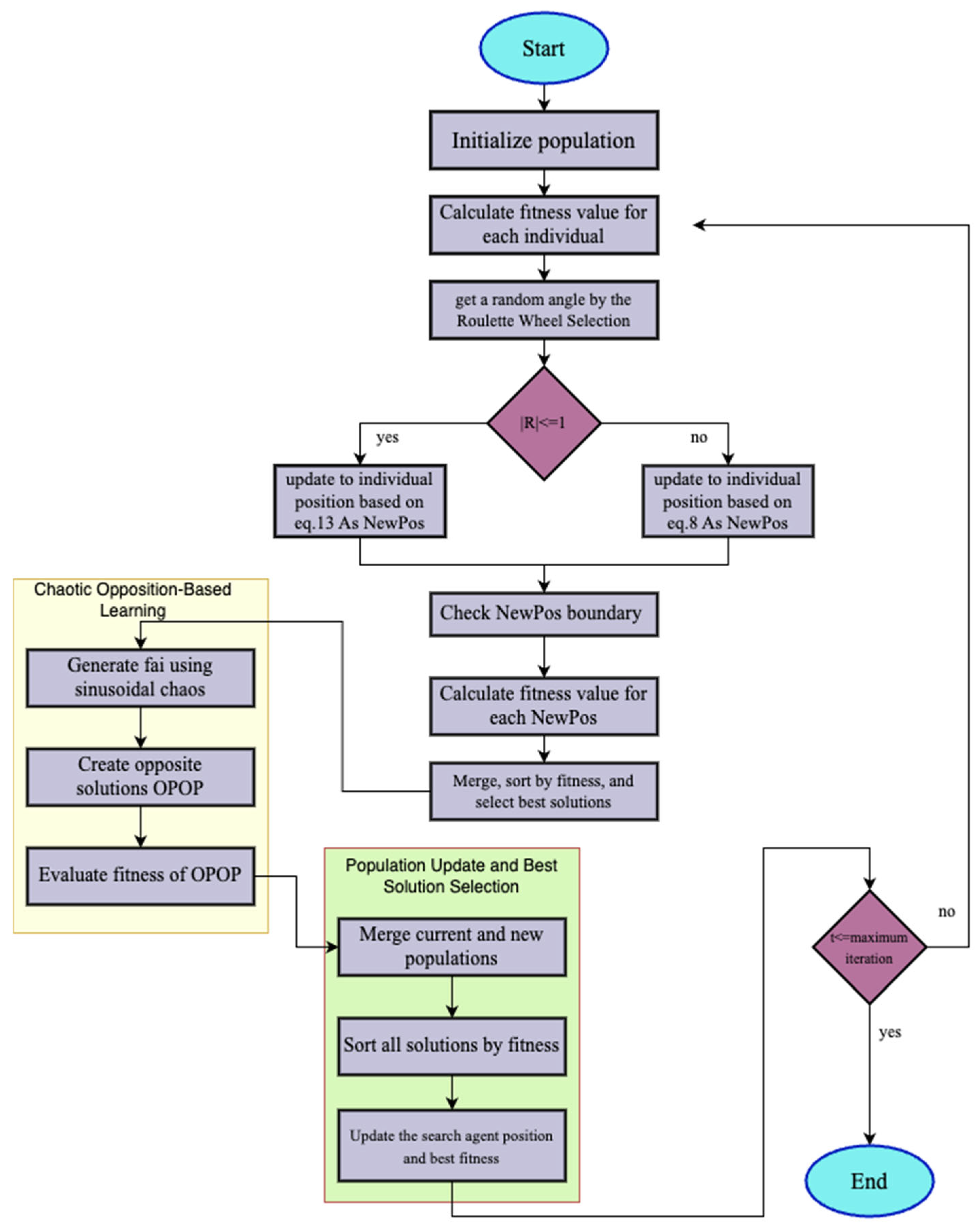
3. Hybrid Metaheuristic Algorithm

Here, the classic SCSO and GWO algorithms are used to propose a new hybrid algorithm that benefits from the advantages of these algorithms to create an efficient algorithm for solving global optimization. In addition, a chaotic opposition-based learning strategy is used in the proposed hybrid optimization algorithm.

3.1. Hybridization SCSO and GWO

The SCSO algorithm uses the R parameter to control the movement of search agents within the search space. This parameter also ensures a balance between exploration and exploitation. Inspired by the unique characteristics of sand cats in nature, the R parameter emphasizes the sensitivity range and decreases from 2 kHz to 0 over time. In contrast, the GWO algorithm uses the A parameter to control the movement of search agents. When the A parameter value is greater or less than 1, it influences the balance between exploration and exploitation. However, this mechanism can lead to drawbacks, such as trapping in local optima, especially in large search spaces. To address this issue, the hybrid algorithm incorporates the R parameter to enhance control over agent movement and improve the balance between exploration and exploitation.

In this context, the COSGO algorithm benefits from the R-value of the SCSO algorithm to switch dynamically between two well-known metaheuristic algorithm strategies. When the R-value is between −1 and 1, the search agents follow the behavior rules of the SCSO algorithm; otherwise, they update their positions based on the GWO algorithm. COSGO also includes a mechanism to validate the fitness of newly updated positions. Updated positions are first checked against the search space boundaries. If they fall outside the allowed limits, correction parameters are applied to move them back within boundaries. Subsequently, a sorting mechanism is employed to merge the new positions with the existing ones, resulting in a combined population of old and new individuals. Likewise, the fitness values of both the existing and new individuals are merged. All individuals are ranked in ascending order based on their fitness values, with the best individual placed at the top. The population is then updated by selecting the top individuals according to the original number of search agents, ensuring that the best solutions are retained.

Grey wolf optimization (GWO) was employed due to its effective global exploration capabilities, simple structure, and minimal parameter requirements, which make it highly adaptable across a variety of optimization problems. On the other hand, the Sand Cat Swarm Optimization (SCSO) algorithm has demonstrated efficient local search behavior and a balanced exploration–exploitation trade-off, making it a suitable candidate for hybridization. The integration of chaotic opposition-based learning further enhances diversity and helps avoid premature convergence. Comparative studies such as [13,14] have also highlighted the complementary strengths of these algorithms, supporting the rationale for their combination in the proposed framework.

3.2. Chaotic Opposition-Based Learning Strategy

One of the recently introduced techniques in optimization is opposition-based learning (OBL) [33]. OBL was first proposed by Tizhoosh to emphasize the evaluation of the opposite position of a search agent within the search space. In this approach, an optimization algorithm evaluates the fitness of both the current position and the opposite position of a search agent. This allows the algorithm to explore the search space more broadly, covering diverse regions and directions. Moreover, in complex optimization problems where multiple local optima exist, search agents can easily become trapped. OBL helps mitigate this issue by increasing the chances of escaping local optima, thus enhancing the global search capability of the algorithm. In Equation (23), which represents the initial population of the optimization algorithm, lb is lower bound, ub is upper bound, and r_i is a random number from a uniform distribution in the range [0, 1]. In equation 24, the opposite position of the current position is calculated:

$$po{s}_{t+1}=Lb+r_i\cdot (Ub-Lb)$$

(23)

$$Opo{s}_{t+1}=Lb+Ub-po{s}_{t+1}$$

(24)

As mentioned earlier, OBL benefits from considering the opposite population based on fixed positions; however, this approach may face limitations. To address this issue, in [34], the authors proposed a modified version of OBL by introducing a random number, which adds a certain level of randomness to the solution and improves diversity. In the chaotic opposition-based learning strategy (COBLS), chaotic behavior is introduced to enhance population diversity and avoid premature convergence. A chaotic array is first generated by iteratively applying the sine map s times. This chaotic array is then used to replace the conventional random array, and opposite solutions are calculated accordingly. As a result, the search process is enriched by exploring different regions of the search space more effectively.

In this study, the sine map was selected as the chaotic map to enhance the diversity of the population during the optimization process. Compared to other chaotic maps such as the Logistic map, the sine map offers smoother and more uniformly distributed sequences, which can help to explore the search space more effectively. Previous studies have shown that the choice of chaotic map can significantly influence the convergence behavior and performance of metaheuristic algorithms [35,36]:

$$Opo{s}_{t+1}=Lb+Ub-F_s ·po{s}_{t+1}$$

(25)

$$F_{i+1}=\mathrm{s}\mathrm{i}\mathrm{n} \left(\pi F_i\right)$$

(26)

In Equation (25), the F_s is a chaotic array that has been mapped using a sine function s times. S is set at 20 in order to prevent the loss of diversity brought on by too few iterations or the increase in running time produced by too many iterations.

3.3. System Model

As aforementioned, this study proposes a new multi-strategy hybrid metaheuristic algorithm to address one of the np-hard problems, multi-level thresholding for color image segmentation. The aim of this problem is to partition a color image into meaningful regions based on pixel intensity values. Initially, it takes an RGB image as input and converts it to greyscale histograms. These histograms are then used to determine the optimal threshold values. This combinatorial optimization problem is modeled, and the goal is to select a set of threshold values that maximizes an image quality criterion. The proposed COSGO algorithm was employed to find these optimal thresholds. To evaluate the COSGO algorithm, a total of 10 real-world images were taken from the BSD500 dataset, which is one of the well-known datasets. The flowchart of the proposed COSGO algorithm is given in Figure 1.

In addition, in the simulation, the main parameters used in the system and COSGO algorithm are explained below:

• T: number of thresholds (3–5 in this study).
• MaxIter: maximum number of iterations (e.g., 100).
• PopulationSize: number of candidate solutions (e.g., 30).
• Objective Functions: Otsu method and Kapur entropy.
• Dataset: BSD500 (10 selected color images).
• Channels: R, G, and B (treated independently for thresholding).
• Evaluation Metric: PSNR, SSIM, and computation time.

It is possible to explain the problem formulation. Let h(i) be an image histogram for intensity level i ∈ [0, 255]. The objective is to determine a threshold vector for a multi-level thresholding problem with T thresholds:

$$T=\left\{t1,t2,\dots ,t_T\right\} with 0<t1<t2<\cdots <t_T<255$$

The goal is to maximize f(T), a fitness function that can be either Otsu’s method or Kapur’s entropy. Thus, the optimization problem is formulated as:

$$\mathit{max}f\left(T\right) subject to t_1<t_2<\cdots <t_T$$

In order to determine the optimal threshold set T that produces the highest segmentation quality based on the chosen objective function, the COSGO algorithm searches the solution space.

4. Results and Analysis

This section evaluates the proposed algorithm using benchmark functions, which are commonly employed to assess metaheuristic algorithms due to their stochastic nature. To demonstrate the effectiveness of the proposed method, it is compared with several metaheuristic algorithms, including GWO [13], SCSO [14], and the WOA [37] and two hybrid metaheuristic algorithms, including AGWO_CS [38] and the PSOGSA [39]. The evaluation includes benchmark tests and statistical analyses. Each algorithm was run independently 30 times using identical control settings, and performance was measured based on the mean and standard deviation. All simulations were conducted on the same system using MATLAB R2020b. The simulation parameters for each metaheuristic algorithm are explained in

Table 1. The simulation parameters.

Algorithm	Parameter	Value	Algorithm	Parameter	Value
GWO	a	[2, 0]	SCSO	Sensitivity range (rG)	[2, 0]
	A	[2, 0]		Phase control range (R)	[−2rG, 2rG]
AGWO_CS	a	$2-\left(cos\left(rand\right)·{\displaystyle \frac{l}{Ma{x}_{iter}}}\right)$	WOA	a	[2, 0]
PSOGSA	$G_0$	1		A	[2, 0]
	C1	0.5		C	2.rand (0, 1)
	C2	1.5		l	[−1, 1]
				b	1

.

4.1. Experimental Analysis Based on CEC2017

For numerical validation, a set of 29 benchmark functions from the CEC2017 test suite was employed, which are widely utilized for assessing the performance of metaheuristic algorithms. These functions are categorized into four groups: the unimodal functions range from F1 to F3, multimodal from F4 to F10, hybrid from F11 to F20, and composite from F21 to F30. The proposed COSGO algorithm was benchmarked using these functions and compared against several existing methods, including GWO, SCSO, the WOA, AGWO-CS, and the PSOGSA.

Table 2. Results for F1-F30 algorithms (CEC17) D10.

Function		COSGO	GWO	SCSO	WOA	AGWO-CS	PSOGSA
F1	Mean	2840	35,700	1.9 × 109	37,800,000	14,600.00	108,000.00
	Worst	8420	54,800	1.92 × 109	1.14 × 109	210,000.00	240,000.00
	Best	126	17,300	1.89 × 109	134	16,600.00	19,500.00
	STD	2380	9430	9,280,000	207,000	38,500.00	45,000.00
F3	Mean	300	1410	2460	877	2520.00	877.00
	Worst	301	4300	27,500	3830	8500.00	3830.00
	Best	300	546	300	302	378.00	302.00
	STD	0.221	960	6000	937	2170.00	937.00
F4	Mean	424	418	421	402	424.00	409.00
	Worst	527	464	529	403	527.00	440.00
	Best	403	407	404	400	403.00	406.00
	STD	27.8	19.8	28.1	0.818	27.80	6.01
F5	Mean	521	520	535	515	521.00	516.00
	Worst	537	542	565	529	537.00	535.00
	Best	510	506	505	508	510.00	504.00
	STD	7.06	10.4	13.4	4.6	7.06	9.11
F6	Mean	600	601	613	613	604.00	601.00
	Worst	600	605	643	640	614.00	605.00
	Best	600	600	602	600	600.00	600.00
	STD	0.0234	1.11	11.4	11.6	3.13	1.08
F7	Mean	719	731	763	724	738.00	734.00
	Worst	729	746	803	749	765.00	756.00
	Best	713	717	730	712	715.00	716.00
	STD	3.52	10	20.5	9.88	12.00	11.10
F8	Mean	812	816	827	834	819.00	817.00
	Worst	824	837	838	857	829.00	835.00
	Best	805	805	814	818	811.00	805.00
	STD	5.41	8.11	7.33	8.04	4.94	7.66
F9	Mean	900	907	997	913	919.00	910.00
	Worst	900	969	1280	970	973.00	984.00
	Best	900	900	903	905	900.00	900.00
	STD	0.0124	14.3	88.8	11.4	24.10	21.70
F10	Mean	1500	1720	1890	1520	1900.00	1480.00
	Worst	2270	2840	2490	2000	2520.00	2500.00
	Best	1000	1180	1240	1250	1420.00	1130.00
	STD	450	412	296	156	308.00	317.00
F11	Mean	1150	1120	1100	1110	1150.00	1130.00
	Worst	1240	1150	1110	1130	1240.00	1310.00
	Best	1120	1100	1100	1100	1120.00	1110.00
	STD	31.3	11.3	2.01	5.82	31.30	44.20
F12	Mean	641,000	948,000	943,000	844,000	641,000.00	844,000.00
	Worst	2,820,000	7,210,000	3,890,000	2,740,000	2,820,000.00	2,740,000.00
	Best	13,200	27,700	46,100	8660	13,200.00	8660.00
	STD	740,000	1,410,000	999,000	901,000	740,000.00	901,000.00
F13	Mean	8300	13,000	11,600	8450	8450.00	12,600.00
	Worst	29,000	26,500	35,100	15,400	15,400.00	29,700.00
	Best	1360	2280	2500	3190	3190.00	3140.00
	STD	7650	7460	8740	2990	2990.00	6760.00
F14	Mean	1450	2900	2100	1470	3060.00	1540.00
	Worst	1480	7240	5230	1560	5560.00	1610.00
	Best	1440	1450	1440	1420	1450.00	1500.00
	STD	11.3	1860	1400	35.2	1740.00	24.00
F15	Mean	1540	4380	2710	1690	5230.00	4120.00
	Worst	1580	10,100	7690	2820	10,600.00	6020.00
	Best	1510	1650	1560	1520	1580.00	1640.00
	STD	16.1	2270	1420	255	2440.00	1150.00
F16	Mean	1770	1820	1800	1780	1770.00	1700.00
	Worst	1990	2240	2000	1960	1990.00	2050.00
	Best	1620	1600	1620	1600	1620.00	1610.00
	STD	118	178	108	111	118.00	115.00
F17	Mean	1760	1760	1760	1790	1760.00	1790.00
	Worst	1870	1890	1820	1880	1870.00	1880.00
	Best	1720	1720	1730	1740	1720.00	1740.00
	STD	34.2	37.1	19.1	34.4	34.20	34.40
F18	Mean	20,800	25,300	18,900	16,100	20,800.00	30,800.00
	Worst	41,200	55,300	50,500	40,900	41,200.00	55,600.00
	Best	3640	4060	2010	2480	3640.00	2930.00
	STD	13,600	13,900	12,500	12,100	13,600.00	16,200.00
F19	Mean	1930	8260	6690	2770	15,400.00	8380.00
	Worst	1970	18,600	14,700	10,100	258,000.00	18,900.00
	Best	1910	1930	1910	1900	1910.00	1920.00
	STD	13.2	6190	5640	1860	46,200.00	6530.00
F20	Mean	2020	2200	2100	2040	2090.00	2060.00
	Worst	2030	2280	2230	2150	2220.00	2150.00
	Best	2000	2180	2040	2000	2030.00	2020.00
	STD	7.51	19.8	55	46	58.40	43.10
F21	Mean	2270	2270	2260	2300	2310.00	2310.00
	Worst	2330	2330	2340	2340	2340.00	2340.00
	Best	2200	2100	2100	2200	2200.00	2200.00
	STD	53.7	63.2	69.6	48.5	30.40	21.70
F22	Mean	2300	2300	2300	2310	2310.00	2310.00
	Worst	2310	2320	2330	2340	2340.00	2330.00
	Best	2200	2220	2250	2300	2300.00	2300.00
	STD	18.7	16	14.1	8.76	8.76	6.33
F23	Mean	2620	2620	2640	2620	2620.00	2620.00
	Worst	2650	2640	2690	2630	2650.00	2650.00
	Best	2610	2600	2620	2610	2610.00	2610.00
	STD	8.73	9.8	14.4	7.75	8.73	11.20
F24	Mean	2750	2730	2750	2740	2750.00	2750.00
	Worst	2800	2780	2820	2780	2800.00	2770.00
	Best	2720	2510	2500	2500	2720.00	2730.00
	STD	14.3	61.8	67	53.5	14.30	13.00
F25	Mean	2930	2940	2940	2930	2930.00	2940.00
	Worst	2950	2950	3020	2950	2950.00	3020.00
	Best	2910	2900	2900	2900	2910.00	2900.00
	STD	13	14.2	22.7	22.8	13.00	22.80
F26	Mean	3040	2930	3010	2940	3040.00	2960.00
	Worst	4060	3190	3470	3830	4060.00	3840.00
	Best	2750	2900	2810	2600	2750.00	2900.00
	STD	289	59.6	128	186	289.00	171.00
F27	Mean	3100	3100	3100	3100	3100.00	3090.00
	Worst	3170	3120	3180	3160	3170.00	3100.00
	Best	3090	3090	3090	3090	3090.00	3090.00
	STD	17.5	5.8	18.6	16.4	17.50	3.02
F28	Mean	3370	3380	3280	3220	3370.00	3370.00
	Worst	3480	3450	3410	3410	3480.00	3410.00
	Best	3170	3180	3160	3100	3170.00	3170.00
	STD	99.7	62.6	109	144	99.70	83.90
F29	Mean	3200	3200	3250	3200	3200.00	3200.00
	Worst	3290	3320	3450	3310	3290.00	3300.00
	Best	3160	3150	3160	3150	3160.00	3140.00
	STD	38.5	50	70.2	44.1	38.50	42.50
F30	Mean	33,200	550,000	464,000	253,000	648,000.00	893,000.00
	Worst	831,000	1,920,000	2,270,000	821,000	6,730,000.00	2,450,000.00
	Best	3820	5430	7120	4520	8600.00	7470.00
	STD	151,000	715,000	658,000	378,000	1,460,000.00	621,000.00

summarizes the experimental outcomes in terms of mean, worst, best, and standard deviation values. In this way, the Friedman ranking presented in

Table 3. Friedman rankings of COSGO and the compared algorithms.

Function	COSGO	GWO	SCSO	WOA	AGWO_CS	PSOGSA
1	1	3	6	5	2	4
3	1	4	5	2.5	6	2.5
4	5	3	4	1	5	2
5	4	3	6	1	4	2
6	1	2.5	5.5	5.5	4	2.5
7	1	3	6	2	5	4
8	1	2	5	6	4	3
9	1	2	6	4	5	3
10	2	4	5	3	6	1
11	5	3	1	2	5	4
12	1.5	6	5	3.5	1.5	3.5
13	1	6	4	2.5	2.5	5
14	1	5	4	2	6	3
15	1	5	3	2	6	4
16	2	6	5	4	2	1
17	2.5	2.5	2.5	5.5	2.5	5.5
18	3	5	2	1	3	6
19	1	4	3	2	6	5
20	1	6	5	2	4	3
21	2.5	2.5	1	4	5.5	5.5
22	2	2	2	5	5	5
23	3	3	6	3	3	3
24	3	1	3	2	3	3
25	2.5	5	5	2.5	2.5	5
26	5.5	1	4	2	5.5	3
27	4	4	4	4	4	1
28	4	6	2	1	4	4
29	3	3	6	3	3	3
30	1	4	3	2	5	6
Total	66.5	106.5	119	85	120	102.5
Average Ranking	2.2931	3.6724	4.1034	2.9310	4.1379	3.5345

was used to compare the performance of COSGO to metaheuristic algorithms. For each benchmark function, the algorithms are ranked based on their performance, with the best-performing algorithm. These rankings were then averaged over all problems to compute the overall Friedman rank for each algorithm. A lower average rank indicates better overall performance. The Friedman test is a non-parametric statistical method that helps determine whether the observed differences in ranks among the algorithms are statistically significant. Based on Table 3, it is observed that the average ranking of the COSGO algorithm is lower than the other algorithms. It means the COSGO algorithm performance is better than the others.

4.2. Experimental Analysis Based on Multi-Level Thresholding

To assess the performance of the proposed COSGO algorithm against other methods, multiple quantitative metrics were used, such as the Peak Signal-to-Noise Ratio (PSNR), the Feature Similarity Index (FSIM), the Structural Similarity Index Measure (SSIM), dice, and the Jaccard index and accuracy, along with the optimal objective function values and their associated variances. In this regard, ten images were selected from the BSD500 dataset [40]. For ease of interpretation and comparative analysis, the best results averaged over 10 independent runs are highlighted in bold in the subsequent tables.

Table 4. The fitness values of the algorithms.

Level	Image		COSGO		GWO		SCSO		WOA		AGWO_CS		PSOGSA
			Otsu	Kapur	Otsu	Kapur	Otsu	Kapur	Otsu	Kapur	Otsu	Kapur	Otsu	Kapur
2	118031	Value	−18,504.54	−5.15	−18,504.54	−5.15	−18,504.54	−5.15	−18,504.51	−5.15	−18,504.32	−5.15	−18,504.54	−5.15
		STD	0.00	0.00	0.00	0.00	0.00	0.00	0.05	0.00	0.15	0.00	0.00	0.00
	118072	Value	−9517.97	−5.04	−9517.97	−5.04	−9517.97	−5.04	−9517.96	−5.04	−9517.91	−5.04	−9517.97	−5.04
		STD	0.00	0.00	0.00	0.00	0.00	0.00	0.02	0.00	0.06	0.00	0.00	0.00
	326025	Value	−6334.31	−4.88	−6334.31	−4.88	−6334.31	−4.88	−6334.31	−4.88	−6334.25	−4.88	−6334.31	−4.88
		STD	0.00	0.00	0.00	0.00	0.00	0.00	0.00	0.00	0.08	0.00	0.00	0.00
	120003	Value	−26,805.11	−5.22	−26,805.11	−5.22	−26,805.11	−5.22	−26,805.08	−5.22	−26,804.92	−5.22	−26,805.11	−5.22
		STD	0.00	0.00	0.00	0.00	0.00	0.00	0.06	0.00	0.05	0.00	0.00	0.00
	253092	Value	−15,027.04	−4.99	−15,027.01	−4.99	−15,027.04	−4.99	−15,027.04	−4.99	−15,026.96	−4.99	−15,027.04	−4.99
		STD	0.00	0.00	0.08	0.00	0.00	0.00	0.01	0.00	0.09	0.00	0.00	0.00
	8068	Value	−12,529.92	−4.65	−12,529.92	−4.65	−12,529.92	−4.65	−12,529.92	−4.65	−12,529.85	−4.65	−12,529.92	−4.65
		STD	0.00	0.00	0.00	0.00	0.00	0.00	0.01	0.00	0.10	0.00	0.00	0.00
	81095	Value	−15,094.56	−5.16	−15,094.56	−5.16	−15,094.56	−5.16	−15,094.56	−5.16	−15,094.53	−5.16	−15,094.56	−5.16
		STD	0.00	0.00	0.00	0.00	0.00	0.00	0.00	0.00	0.06	0.00	0.00	0.00
	92014	Value	−14,961.03	−4.55	−14,961.03	−4.55	−14,961.03	−4.55	−14,961.03	−4.55	−14,960.91	−4.55	−14,961.03	−4.55
		STD	0.00	0.00	0.00	0.00	0.00	0.00	0.01	0.00	0.13	0.00	0.00	0.00
	365072	Value	−17,439.29	−5.48	−17,439.29	−5.48	−17,439.29	−5.48	−17,439.29	−5.48	−17,439.23	−5.48	−17,439.29	−5.48
		STD	0.00	0.00	0.00	0.00	0.00	0.00	0.00	0.00	0.09	0.00	0.00	0.00
	384022	Value	−15,896.95	−5.16	−15,896.95	−5.16	−15,896.95	−5.16	−15,896.93	−5.16	−15,896.90	−5.16	−15,896.95	−5.16
		STD	0.00	0.00	0.00	0.00	0.00	0.00	0.05	0.00	0.03	0.00	0.00	0.00
3	118031	Value	−18,730.87	−5.15	−18,730.74	−5.15	−18,730.87	−5.15	−18,730.84	−5.15	−18,730.08	−5.15	−18,730.87	−5.15
		STD	0.00	0.00	0.29	0.00	0.00	0.00	0.05	0.00	0.33	0.00	0.00	0.00
	118072	Value	−9640.56	−5.04	−9640.56	−5.04	−9640.54	−5.04	−9640.52	−5.04	−9639.99	−5.04	−9640.56	−5.04
		STD	0.00	0.00	0.00	0.00	0.04	0.00	0.05	0.00	0.31	0.00	0.00	0.00
	326025	Value	−6504.93	−4.88	−6504.93	−4.88	−6504.92	−4.88	−6504.85	−4.88	−6504.16	−4.88	−6504.93	−4.88
		STD	0.00	0.00	0.00	0.00	0.01	0.00	0.09	0.00	0.87	0.00	0.00	0.00
	120003	Value	−27,071.72	−5.22	−27,071.70	−5.22	−27,071.71	−5.22	−27,071.54	−5.22	−27,070.76	−5.22	−27,071.72	−5.22
		STD	0.00	0.00	0.04	0.00	0.03	0.00	0.40	0.00	0.94	0.00	0.00	0.00
	253092	Value	−15,184.31	−4.99	−15,183.55	−4.99	−15,184.31	−4.99	−15,184.30	−4.99	−15,183.08	−4.99	−15,184.31	−4.99
		STD	0.00	0.00	1.67	0.00	0.00	0.00	0.01	0.00	0.85	0.00	0.00	0.00
	8068	Value	−12,611.96	−4.65	−12,611.96	−4.65	−12,611.96	−4.65	−12,611.91	−4.65	−12,611.23	−4.65	−12,611.96	−4.65
		STD	0.00	0.00	0.00	0.00	0.00	0.00	0.09	0.00	0.55	0.00	0.00	0.00
	81095	Value	−15,261.54	−5.16	−15,261.38	−5.16	−15,261.53	−5.16	−15,261.44	−5.16	−15,260.17	−5.16	−15,261.54	−5.16
		STD	0.00	0.00	0.35	0.00	0.02	0.00	0.11	0.00	0.66	0.00	0.00	0.00
	92014	Value	−15,071.07	−4.55	−15,070.85	−4.55	−15,071.09	−4.55	−15,071.08	−4.55	−15,070.23	−4.55	−15,071.09	−4.55
		STD	0.04	0.00	0.55	0.00	0.00	0.00	0.02	0.00	0.76	0.00	0.01	0.00
	365072	Value	−17,685.43	−5.48	−17,685.43	−5.48	−17,685.42	−5.48	−17,685.34	−5.48	−17,684.14	−5.48	−17,685.43	−5.48
		STD	0.00	0.00	0.00	0.00	0.03	0.00	0.13	0.00	1.18	0.00	0.00	0.00
	384022	Value	−16,124.65	−5.16	−16,124.65	−5.16	−16,124.65	−5.16	−16,124.62	−5.16	−16,123.64	−5.16	−16,124.65	−5.16
		STD	0.00	0.00	0.00	0.00	0.01	0.00	0.04	0.00	0.77	0.00	0.00	0.00
4	118031	Value	−18,805.074	−5.152	−18,804.707	−5.152	−18,805.081	−5.152	−18,804.720	−5.152	−18,801.351	−5.152	−18,805.082	−5.152
		STD	0.009	0.000	0.845	0.000	0.020	0.000	0.394	0.000	2.147	0.000	0.011	0.000
	118072	Value	−9695.921	−5.036	−9695.365	−5.036	−9695.908	−5.036	−9695.822	−5.036	−9693.808	−5.036	−9695.941	−5.036
		STD	0.019	0.000	1.271	0.000	0.040	0.000	0.164	0.000	1.821	0.000	0.000	0.000
	326025	Value	−6593.882	−4.885	−6593.882	−4.885	−6593.886	−4.885	−6593.854	−4.885	−6592.268	−4.885	−6593.886	−4.885
		STD	0.014	0.000	0.014	0.000	0.005	0.000	0.044	0.000	1.137	0.000	0.005	0.000
	120003	Value	−27,163.825	−5.220	−27,163.808	−5.220	−27,163.801	−5.220	−27,163.555	−5.220	−27,161.155	−5.220	−27,163.828	−5.220
		STD	0.003	0.000	0.038	0.000	0.054	0.000	0.244	0.000	1.277	0.000	0.000	0.000
	253092	Value	−15,254.533	−4.990	−15,254.046	−4.990	−15,254.540	−4.990	−15,254.434	−4.990	−15,252.271	−4.990	−15,254.543	−4.990
		STD	0.015	0.000	1.078	0.000	0.008	0.000	0.105	0.000	1.013	0.000	0.000	0.000
	8068	Value	−12,666.569	−4.645	−12,666.569	−4.645	−12,666.571	−4.645	−12,666.394	−4.645	−12,664.976	−4.645	−12,662.381	−4.645
		STD	0.004	0.000	0.004	0.000	0.000	0.000	0.215	0.000	1.148	0.000	9.369	0.000
	81095	Value	−15,321.807	−5.156	−15,321.806	−5.156	−15,321.817	−5.156	−15,321.695	−5.156	−15,320.714	−5.156	−15,321.807	−5.156
		STD	0.028	0.000	0.031	0.000	0.023	0.000	0.161	0.000	0.590	0.000	0.028	0.000
	92014	Value	−15,132.280	−4.552	−15,132.276	−4.552	−15,132.281	−4.552	−15,132.270	−4.552	−15,129.595	−4.552	−15,132.276	−4.552
		STD	0.005	0.000	0.006	0.000	0.005	0.000	0.031	0.000	1.515	0.000	0.007	0.000
	365072	Value	−17,791.010	−5.483	−17,790.996	−5.483	−17,791.033	−5.483	−17,790.846	−5.483	−17,787.168	−5.483	−17,791.008	−5.483
		STD	0.032	0.000	0.051	0.000	0.000	0.000	0.275	0.000	1.619	0.000	0.041	0.000
	384022	Value	−16,180.251	−5.160	−16,180.238	−5.160	−16,169.119	−5.160	−16,179.835	−5.160	−16,177.785	−5.160	−16,179.035	−5.160
		STD	0.009	0.000	0.009	0.000	24.859	0.000	0.661	0.000	1.126	0.000	2.727	0.000
5	118031	Value	−18,843.8	−5.15164	−1.88 × 104	−5.15 × 100	−18,836	−5.15164	−18,843.5	−5.15164	−18,843.8	−5.15164	−1.88 × 104	−5.15 × 100
		STD	0.024575	0	2.185805	6.28 × 10−16	17.26396	0	0.432428	0	0.024575	0	2.185805	6.28 × 10−16
	118072	Value	−9.73 × 103	−5.04 × 100	−9.72 × 103	−5.04 × 100	−9.72 × 103	−5.04 × 100	−9.73 × 103	−5.04 × 100	−9.73 × 103	−5.04 × 100	−9.72 × 103	−5.04 × 100
		STD	0.015209	8.88 × 10−16	1.713792	4.44 × 10−16	13.31547	4.44 × 10−16	0.437801	8.88 × 10−16	0.015209	8.88 × 10−16	1.713792	4.44 × 10−16
	326025	Value	−6640.82	−4.88486	−6.64 × 103	−4.88 × 100	−6.64 × 103	−4.88 × 100	−6.64 × 103	−4.88 × 100	−6640.82	−4.88486	−6.64 × 103	−4.88 × 100
		STD	0.02325	0	0.000355	6.28 × 10−16	0.007064	7.69 × 10−16	0.321744	7.69 × 10−16	0.02325	0	0.000355	6.28 × 10−16
	120003	Value	−2.72 × 104	−5.22 × 100	−2.72 × 104	−5.22 × 100	−2.72 × 104	−5.22 × 100	−27,219.5	−5.21957	−2.72 × 104	−5.22 × 100	−2.72 × 104	−5.22 × 100
		STD	0.062141	7.69 × 10−16	0.138989	8.88 × 10−16	0.239523	8.88 × 10−16	1.980433	0	0.062141	7.69 × 10−16	0.138989	8.88 × 10−16
	253092	Value	−1.53 × 104	−4.99 × 100	−15,292.5	−4.99043	−15,293.9	−4.99043	−15,285.9	−4.99043	−1.53 × 104	−4.99 × 100	−15,292.5	−4.99043
		STD	0.088749	4.44 × 10−16	3.140839	0	0.001474	0	17.53074	0	0.088749	4.44 × 10−16	3.140839	0
	8068	Value	−1.27 × 104	−4.65 × 100	−1.27 × 104	−4.65 × 100	−1.27 × 104	−4.65 × 100	−1.27 × 104	−4.65 × 100	−1.27 × 104	−4.65 × 100	−1.27 × 104	−4.65 × 100
		STD	0.005499	4.44 × 10−16	2.946929	4.44 × 10−16	0.022274	1.09 × 10−15	0.901476	8.88 × 10−16	0.005499	4.44 × 10−16	2.946929	4.44 × 10−16
	81095	Value	−1.54 × 104	−5.16 × 100	−1.54 × 104	−5.16 × 100	−1.54 × 104	−5.16 × 100	−1.54 × 104	−5.16 × 100	−1.54 × 104	−5.16 × 100	−1.54 × 104	−5.16 × 100
		STD	0.006642	7.69 × 10−16	0.421632	4.44 × 10−16	16.24358	6.28 × 10−16	0.66682	4.44 × 10−16	0.006642	7.69 × 10−16	0.421632	4.44 × 10−16
	92014	Value	−1.52 × 104	−4.55 × 100	−15,159.7	−4.55222	−1.52 × 104	−4.55 × 100	−15,160.5	−4.55222	−1.52 × 104	−4.55 × 100	−15,159.7	−4.55222
		STD	0.057762	6.28 × 10−16	1.830489	0	0.017674	4.44 × 10−16	0.052781	0	0.057762	6.28 × 10−16	1.830489	0
	365072	Value	−1.78 × 104	−5.48 × 100	−17,848.9	−5.48253	−1.78 × 104	−5.48 × 100	−1.78 × 104	−5.48 × 100	−1.78 × 104	−5.48 × 100	−17,848.9	−5.48253
		STD	0.036263	4.44 × 10−16	0.030867	0	0.116513	1.09 × 10−15	0.150933	8.88 × 10−16	0.036263	4.44 × 10−16	0.030867	0
	384022	Value	−1.62 × 104	−5.16 × 100	−16,225.7	−5.16025	−1.62 × 104	−5.16 × 100	−16,226	−5.16025	−1.62 × 104	−5.16 × 100	−16,225.7	−5.16025
		STD	0.020737	6.28 × 10−16	2.203184	0	0.211542	4.44 × 10−16	0.704882	0	0.020737	6.28 × 10−16	2.203184	0

presents the average and standard deviation fitness function values for all compared methods across thresholding levels 2, 3, 4, and 5 evaluated on all images using two objective functions: Otsu’s method and Kapur’s entropy. Moreover, the proposed COSGO algorithm demonstrates lower computational time at threshold level 2 and level 3. Based on the obtained results of the running time of each algorithm, which are presented in

Table 5. The running time of each algorithm.

Level	Image	COSGO		GWO		SCSO		WOA		AGWO_CS		PSOGSA
		Otsu	Kapur	Otsu	Kapur	Otsu	Kapur	Otsu	Kapur	Otsu	Kapur	Otsu	Kapur
2	118031	0.8769	0.9559	0.2855	0.3186	0.2969	0.3218	0.2884	0.3146	0.3003	0.3298	0.2900	0.3198
	118072	0.8331	0.9563	0.2861	0.3181	0.2898	0.3223	0.2802	0.3136	0.2966	0.3290	0.2842	0.3195
	326025	0.8368	0.9590	0.2862	0.3197	0.2938	0.3225	0.2825	0.3143	0.2943	0.3316	0.2940	0.3191
	120003	0.8435	0.9637	0.2842	0.3189	0.2879	0.3268	0.2821	0.3152	0.2973	0.3295	0.2824	0.3220
	253092	0.8432	0.9507	0.2859	0.3173	0.2913	0.3215	0.2791	0.3101	0.2938	0.3275	0.2840	0.3171
	8068	0.8437	0.9573	0.2831	0.3190	0.2913	0.3236	0.2809	0.3133	0.2930	0.3292	0.2878	0.3189
	81095	0.8351	0.9547	0.2794	0.3187	0.2902	0.3253	0.2815	0.3117	0.2932	0.3295	0.2949	0.3202
	92014	0.8507	0.9520	0.2860	0.3181	0.2919	0.3254	0.2846	0.3135	0.2951	0.3307	0.2859	0.3193
	365072	0.8325	0.9484	0.2786	0.3162	0.2830	0.3203	0.2828	0.3104	0.2919	0.3273	0.2839	0.3181
	384022	0.8334	0.9470	0.2813	0.3272	0.2872	0.3237	0.2815	0.3144	0.2912	0.3306	0.2899	0.3201
3	118031	0.8883	0.9767	0.2931	0.3254	0.2945	0.3329	0.2934	0.3228	0.3139	0.3457	0.2949	0.3223
	118072	0.8539	0.9695	0.2835	0.3258	0.2935	0.3288	0.2843	0.3256	0.3030	0.3432	0.2874	0.3237
	326025	0.8739	0.9839	0.2876	0.3290	0.2912	0.3324	0.2929	0.3260	0.3068	0.3430	0.2976	0.3245
	120003	0.8653	0.9769	0.2879	0.3265	0.2934	0.3373	0.2887	0.3277	0.3056	0.3451	0.2912	0.3251
	253092	0.8573	0.9601	0.2892	0.3198	0.2933	0.3295	0.2886	0.3206	0.3025	0.3352	0.2895	0.3199
	8068	0.8559	0.9788	0.2886	0.3257	0.2950	0.3330	0.2853	0.3247	0.3066	0.3376	0.2958	0.3290
	81095	0.8618	0.9609	0.2858	0.3259	0.2942	0.3347	0.2907	0.3215	0.3045	0.3396	0.2978	0.3251
	92014	0.8698	0.9725	0.2877	0.3270	0.2952	0.3323	0.2850	0.3238	0.3080	0.3436	0.2950	0.3256
	365072	0.8560	0.9618	0.2847	0.3252	0.2915	0.3322	0.2835	0.3212	0.3022	0.3418	0.2869	0.3213
	384022	0.8608	0.9753	0.2856	0.3246	0.2891	0.3333	0.2842	0.3265	0.3028	0.3391	0.2866	0.3258
4	118031	0.9017	1.0080	0.2921	0.3369	0.2969	0.3355	0.2897	0.3271	0.3137	0.3503	0.3019	0.3348
	118072	0.8971	0.9984	0.2908	0.3428	0.2975	0.3410	0.2858	0.3339	0.3101	0.3500	0.2942	0.3341
	326025	0.8771	1.0022	0.2892	0.3335	0.2933	0.3361	0.2896	0.3365	0.3105	0.3519	0.2980	0.3373
	120003	0.8722	0.9890	0.2991	0.3349	0.3004	0.3394	0.2889	0.3338	0.3160	0.3533	0.2955	0.3375
	253092	0.8793	0.9681	0.2998	0.3309	0.2947	0.3412	0.2890	0.3299	0.3079	0.3503	0.2948	0.3290
	8068	0.8901	0.9726	0.2894	0.3327	0.2974	0.3363	0.2852	0.3265	0.3094	0.3488	0.3010	0.3295
	81095	0.8797	0.9799	0.2907	0.3320	0.2980	0.3343	0.2864	0.3278	0.3073	0.3491	0.3021	0.3356
	92014	0.8896	1.0001	0.2932	0.3307	0.2961	0.3505	0.2912	0.3269	0.3113	0.3579	0.3006	0.3328
	365072	0.8610	0.9931	0.2892	0.3348	0.2938	0.3334	0.2892	0.3334	0.3063	0.3501	0.2931	0.3297
	384022	0.8790	0.9992	0.3008	0.3340	0.2968	0.3365	0.2919	0.3298	0.3055	0.3489	0.2950	0.3353
5	118031	0.8970	0.9917	0.3113	0.3451	0.3047	0.3399	0.2965	0.3275	0.3205	0.3559	0.3045	0.3325
	118072	0.8763	0.9898	0.3134	0.3415	0.2968	0.3365	0.2899	0.3288	0.3092	0.3631	0.2958	0.3310
	326025	0.8902	0.9990	0.3129	0.3465	0.3018	0.3399	0.2882	0.3254	0.3146	0.3597	0.3013	0.3326
	120003	0.8857	0.9936	0.3203	0.3486	0.3007	0.3337	0.2918	0.3315	0.3131	0.3546	0.3006	0.3329
	253092	0.9002	0.9818	0.3062	0.3390	0.2965	0.3347	0.2892	0.3282	0.3155	0.3731	0.2979	0.3289
	8068	0.8874	0.9833	0.3024	0.3401	0.2985	0.3323	0.2890	0.3261	0.3134	0.3605	0.3014	0.3330
	81095	0.8722	0.9910	0.3097	0.3348	0.2964	0.3393	0.2885	0.3291	0.3174	0.3679	0.3039	0.3286
	92014	0.8786	0.9942	0.3070	0.3421	0.2971	0.3399	0.2921	0.3394	0.3151	0.3699	0.2996	0.3276
	365072	0.8606	0.9963	0.2984	0.3395	0.2974	0.3364	0.2875	0.3285	0.3072	0.3522	0.2987	0.3273
	384022	0.8866	1.0177	0.2969	0.3346	0.2936	0.3376	0.2860	0.3283	0.3098	0.3548	0.2972	0.3271

, the COSGO algorithm achieves superior performance in terms of execution time.

The segmentation results based on Otsu and Kapur entropy are shown in

Table 6. The PSNR and MSE values of the algorithms.

Level	Image		COSGO		GWO		SCSO		WOA		AGWO_CS		PSOGSA
			Otsu	Kapur	Otsu	Kapur	Otsu	Kapur	Otsu	Kapur	Otsu	Kapur	Otsu	Kapur
2	118031	PSNR	19.51	16.14	19.51	16.76	19.51	16.23	19.50	16.47	19.42	15.46	19.51	16.18
		MSE	727.94	1603.79	727.94	1416.16	727.94	1561.26	729.86	1484.20	743.18	1919.64	727.94	1588.24
	118072	PSNR	19.54	16.80	19.54	17.66	19.54	17.91	19.54	16.87	19.54	15.06	19.54	17.08
		MSE	723.02	1498.45	723.02	1225.43	723.02	1223.50	723.09	1420.47	723.36	2130.41	723.02	1317.66
	326025	PSNR	21.54	19.70	21.54	16.26	21.54	15.33	21.55	16.04	21.54	16.87	21.54	15.22
		MSE	455.85	761.11	455.85	2075.13	455.85	2277.03	455.55	1862.70	456.18	1659.86	455.85	3026.49
	120003	PSNR	20.21	14.85	20.21	14.55	20.21	13.83	20.20	15.55	20.16	12.44	20.21	16.58
		MSE	619.69	2412.10	619.69	2619.17	619.69	2693.16	620.89	2017.50	627.36	4020.18	619.69	1658.73
	253092	PSNR	15.16	14.42	15.16	14.35	15.16	14.35	15.17	14.17	15.17	13.81	15.16	14.81
		MSE	1981.66	2378.72	1979.69	2411.36	1981.66	2393.70	1979.08	2519.82	1975.38	2721.10	1981.66	2152.47
	8068	PSNR	16.14	10.55	16.14	10.55	16.14	11.46	16.14	10.95	16.14	10.55	16.14	12.04
		MSE	1582.45	5747.19	1582.45	5737.83	1582.45	4724.23	1582.64	5410.56	1583.09	5919.62	1582.45	4177.89
	81095	PSNR	20.00	15.64	20.00	16.07	20.00	16.52	20.00	16.84	19.99	14.97	20.00	15.98
		MSE	649.97	1775.69	649.97	1667.19	649.97	1506.76	649.97	1375.75	651.71	2083.89	649.97	1668.81
	92014	PSNR	9.74	9.59	9.74	9.45	9.74	9.52	9.75	9.43	9.75	9.51	9.74	9.43
		MSE	6898.32	7156.04	6898.32	7382.34	6898.32	7269.33	6895.70	7433.11	6894.52	7287.66	6898.32	7432.31
	365072	PSNR	20.67	12.86	20.67	12.53	20.67	13.04	20.67	14.42	20.66	13.50	20.67	16.95
		MSE	557.46	3465.46	557.46	3683.50	557.46	3291.42	557.46	2572.63	558.16	3347.27	557.46	1614.96
	384022	PSNR	19.93	16.89	19.93	16.40	19.93	17.29	19.92	17.97	19.94	15.85	19.93	16.72
		MSE	661.26	1426.22	661.26	1589.15	661.26	1283.28	661.92	1091.16	659.15	1795.36	661.26	1527.68
3	118031	PSNR	22.9351	16.1268	22.9395	16.8132	22.9351	17.8432	22.9771	16.4218	23.0017	17.0766	22.9351	16.7904
		MSE	330.8066	1587.5032	330.4663	1388.9745	330.8066	1081.3988	327.6347	1500.8736	325.8938	1308.5358	330.8066	1450.2195
	118072	PSNR	21.8671	19.0321	21.8671	20.4082	21.8688	20.8823	21.8721	18.7467	21.8783	18.3972	21.8671	18.8232
		MSE	423.0325	857.9918	423.0325	609.7335	422.8679	573.7079	422.5413	921.7215	422.3121	1254.7416	423.0325	954.7287
	326025	PSNR	24.0745	19.5266	24.0745	19.2204	24.0684	19.6495	24.0650	18.1740	24.0191	18.6720	24.0745	18.4796
		MSE	254.4667	768.5329	254.4667	947.5201	254.8246	754.1504	255.0223	1163.7450	257.7481	978.2080	254.4667	970.3092
	120003	PSNR	23.5687	17.2643	23.5664	17.9989	23.5678	18.3603	23.5650	16.6042	23.5177	13.9925	23.5687	19.9053
		MSE	285.8943	1519.4354	286.0463	1195.9356	285.9580	1040.8176	286.1398	1836.8011	289.2805	2599.2134	285.8943	697.5528
	253092	PSNR	15.6191	14.2779	15.6303	15.1022	15.6191	15.1786	15.6193	14.7340	15.5954	14.6339	15.6191	14.9065
		MSE	1783.0651	2450.0577	1778.4972	2014.7354	1783.0651	1985.2576	1783.0104	2188.1618	1792.8673	2267.9789	1783.0651	2107.3803
	8068	PSNR	16.4546	11.0887	16.4546	12.5159	16.4546	11.8508	16.4526	11.2104	16.4597	10.1321	16.4546	12.1029
		MSE	1471.0292	5093.5785	1471.0292	3961.2185	1471.0292	4329.9797	1471.6988	4978.9180	1469.3146	6633.4375	1471.0292	4327.0509
	81095	PSNR	23.5034	15.8988	23.4930	15.9230	23.5235	16.9943	23.5246	18.2818	23.5496	16.2688	23.5034	18.4466
		MSE	290.2267	1679.0968	290.9304	1693.7111	288.9014	1403.3690	288.8323	1116.9040	287.1832	1618.6846	290.2267	1002.2381
	92014	PSNR	9.9854	9.8244	9.9835	9.8756	9.9855	9.6024	9.9837	9.6813	9.9798	9.8877	9.9854	9.6678
		MSE	6524.4049	6773.2089	6527.2132	6691.6330	6524.1913	7135.6674	6527.0265	7000.3487	6532.7637	6674.3300	6524.3526	7024.2659
	365072	PSNR	23.2644	13.1461	23.2644	15.3812	23.2635	14.4680	23.2638	12.3608	23.2482	15.9268	23.2644	19.0736
		MSE	306.6449	3344.1274	306.6449	2150.0121	306.7088	2687.2560	306.6893	3777.8059	307.7983	2194.2999	306.6449	1173.5723
	384022	PSNR	24.6464	16.2940	24.6464	17.2054	24.6443	18.0827	24.6481	16.4700	24.6232	17.7313	24.6464	18.0721
		MSE	223.0680	1558.4437	223.0680	1277.8032	223.1773	1046.8039	222.9844	1499.4587	224.2729	1210.3236	223.0680	1060.0297
4	118031	PSNR	24.53	17.50	24.56	18.93	24.52	17.82	24.54	17.66	24.48	15.88	24.53	18.40
		MSE	229.08	1177.38	227.77	922.91	229.69	1135.00	228.78	1131.68	232.16	1716.31	228.92	1005.15
	118072	PSNR	24.03	19.06	24.02	21.97	23.99	20.34	24.08	21.37	23.93	19.97	24.02	19.57
		MSE	256.87	935.98	257.66	438.79	259.48	658.31	254.19	638.95	263.56	807.32	257.63	876.66
	326025	PSNR	25.98	22.17	25.98	19.93	25.97	19.83	25.98	21.05	25.94	17.46	25.97	19.21
		MSE	164.02	422.00	164.02	880.27	164.37	742.25	164.04	542.57	165.60	2176.26	164.37	926.52
	120003	PSNR	25.26	16.71	25.26	20.61	25.27	17.52	25.25	19.97	25.20	13.14	25.27	18.46
		MSE	193.71	1893.83	193.61	621.12	193.38	1472.89	193.96	670.40	196.22	3350.84	193.18	1321.95
	253092	PSNR	15.98	15.10	15.96	15.38	15.98	15.46	15.97	14.58	15.89	14.46	15.98	15.04
		MSE	1642.72	2017.10	1649.54	1898.59	1642.61	1854.57	1643.00	2306.10	1673.70	2356.26	1642.55	2066.07
	8068	PSNR	16.46	10.98	16.46	12.07	16.46	13.60	16.47	11.64	16.45	9.96	16.49	12.68
		MSE	1469.12	5234.30	1469.12	4248.12	1468.47	3167.39	1466.01	4648.60	1472.55	6886.64	1459.92	3715.07
	81095	PSNR	24.88	16.57	24.86	19.58	24.88	17.47	24.87	19.15	24.86	16.86	24.88	17.32
		MSE	211.34	1514.17	212.51	780.56	211.52	1278.55	211.78	868.95	212.49	1527.53	211.34	1352.85
	92014	PSNR	10.10	9.83	10.10	9.97	10.10	10.05	10.10	9.65	10.10	9.88	10.10	9.85
		MSE	6356.41	6772.50	6356.94	6554.16	6356.25	6424.65	6356.11	7058.70	6355.09	6686.68	6357.70	6727.22
	365072	PSNR	25.18	12.72	25.18	17.39	25.19	14.90	25.18	16.82	25.09	13.95	25.18	17.74
		MSE	197.06	3535.42	197.19	1317.40	196.95	2608.09	197.43	1726.96	201.56	2873.21	197.15	1578.84
	384022	PSNR	25.61	16.98	25.64	19.43	25.37	20.50	25.52	17.88	25.52	17.29	25.66	20.30
		MSE	178.72	1321.67	177.47	884.30	189.47	672.84	182.51	1193.42	182.59	1274.93	176.83	699.73
5	118031	PSNR	26.05	18.60	26.05	20.34	26.14	18.51	26.16	21.66	25.96	18.63	26.02	19.27
		MSE	161.68	1008.74	161.58	648.90	158.23	1011.57	157.78	469.07	165.38	1037.91	162.54	865.14
	118072	PSNR	25.69	20.56	25.62	21.42	25.63	20.81	25.61	21.68	24.97	21.34	25.57	23.31
		MSE	175.60	681.95	178.19	495.47	178.10	694.31	178.67	449.19	208.81	504.80	180.20	315.30
	326025	PSNR	27.63	19.80	27.63	22.53	27.63	18.87	27.61	22.49	27.39	20.11	27.64	22.14
		MSE	112.25	1023.23	112.18	395.52	112.23	1243.14	112.68	403.09	118.59	651.54	111.92	460.49
	120003	PSNR	26.94	18.99	26.94	19.30	26.93	14.72	26.92	17.39	26.67	14.10	26.91	21.18
		MSE	131.66	846.31	131.44	998.71	131.75	2343.70	132.24	1702.88	139.94	2545.59	132.34	541.65
	253092	PSNR	16.24	15.11	16.23	15.70	16.23	15.07	16.21	15.46	16.26	14.95	16.20	15.51
		MSE	1544.16	2021.33	1550.36	1770.17	1547.55	2028.60	1554.61	1856.85	1537.96	2106.70	1561.64	1850.45
	8068	PSNR	16.62	11.69	16.62	14.12	16.62	13.98	16.61	12.71	16.63	10.85	16.63	13.34
		MSE	1414.48	4476.09	1414.45	2726.31	1414.55	2954.99	1418.46	3795.22	1413.46	5740.31	1413.74	3287.62
	81095	PSNR	26.48	16.31	26.49	22.07	26.41	19.98	26.43	21.23	25.98	15.40	26.09	18.99
		MSE	146.24	1534.75	145.93	428.28	148.49	779.80	148.11	630.37	164.10	1958.40	161.68	952.29
	92014	PSNR	10.15	9.72	10.14	9.87	10.15	9.81	10.14	9.94	10.15	9.94	10.15	9.82
		MSE	6285.96	6942.66	6289.18	6701.73	6287.07	6793.33	6298.67	6598.72	6288.24	6592.38	6288.95	6772.64
	365072	PSNR	26.74	14.63	26.72	18.40	26.74	16.99	26.71	16.60	26.51	16.14	26.74	19.83
		MSE	137.74	2659.72	138.39	1148.47	137.89	1879.41	138.57	1962.17	145.11	2454.43	137.72	747.78
	384022	PSNR	27.16	18.26	27.16	20.40	27.12	21.67	26.82	16.89	26.85	19.13	27.12	21.90
		MSE	125.14	1058.45	125.01	655.66	126.19	502.82	136.74	1398.76	134.34	1062.81	126.24	605.26

, along with the PSNR, SSIM, and FSIM values. A traditional statistic for assessing image quality is the PSNR. It determines how segmented and original photos differ from one another. The segmented image is more like the original when the PSNR value is higher. In this way, the higher value of the PSNR proves the algorithm efficiently. In addition, the mean square error (MSE) was calculated for each algorithm with two objective functions. The obtained results were also in the same running condition, with 100 iteration numbers and 30 search agent numbers. It was observed that the proposed COSGO algorithm showed better performance in terms of higher PSNR and lower MSE values in comparison to the other algorithms.

The Structural Similarity Index Measure (SSIM) evaluates the perceived quality of an image by incorporating luminance, contrast, and structural information. A higher SSIM value closer to 1 indicates a greater structural similarity between the segmented image and the original image. The Feature Similarity Index Measure (FSIM), which is widely used for image quality assessment, particularly in terms of texture and detail preservation, quantifies the similarity based on low-level image features, such as phase congruency and gradient magnitude.

Table 7. The SSIM and FSIM values of the algorithms.

Level	Image		COSGO		GWO		SCSO		WOA		AGWO_CS		PSOGSA
			Otsu	Kapur	Otsu	Kapur	Otsu	Kapur	Otsu	Kapur	Otsu	Kapur	Otsu	Kapur
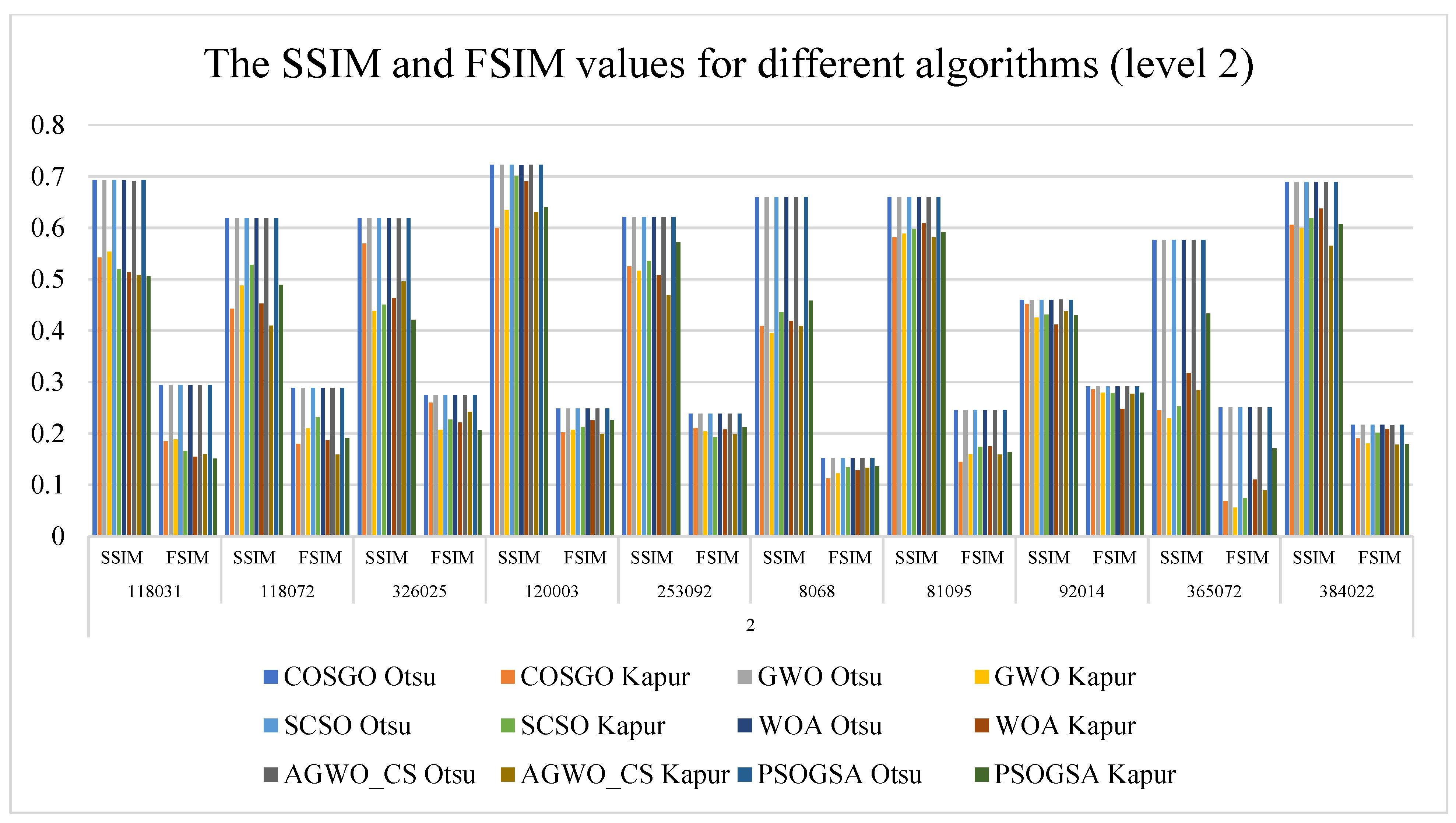
2	118031	SSIM	0.6929	0.5421	0.6929	0.5533	0.6929	0.5196	0.6928	0.5139	0.6914	0.5079	0.6929	0.5061
		FSIM	0.2940	0.1850	0.2940	0.1880	0.2940	0.1657	0.2939	0.1546	0.2934	0.1595	0.2940	0.1507
	118072	SSIM	0.6188	0.4424	0.6188	0.4880	0.6188	0.5280	0.6188	0.4528	0.6188	0.4095	0.6188	0.4891
		FSIM	0.2884	0.1795	0.2884	0.2099	0.2884	0.2310	0.2886	0.1866	0.2889	0.1587	0.2884	0.1906
	326025	SSIM	0.6185	0.5693	0.6185	0.4385	0.6185	0.4504	0.6185	0.4638	0.6179	0.4957	0.6185	0.4215
		FSIM	0.2750	0.2596	0.2750	0.2068	0.2750	0.2267	0.2749	0.2212	0.2744	0.2418	0.2750	0.2058
	120003	SSIM	0.7224	0.5991	0.7224	0.6345	0.7224	0.7003	0.7222	0.6900	0.7223	0.6302	0.7224	0.6400
		FSIM	0.2486	0.2017	0.2486	0.2066	0.2486	0.2126	0.2487	0.2256	0.2487	0.1988	0.2486	0.2258
	253092	SSIM	0.6207	0.5251	0.6204	0.5164	0.6207	0.5360	0.6206	0.5077	0.6200	0.4693	0.6207	0.5718
		FSIM	0.2382	0.2104	0.2381	0.2039	0.2382	0.1926	0.2382	0.2076	0.2381	0.1985	0.2382	0.2117
	8068	SSIM	0.6597	0.4088	0.6597	0.3951	0.6597	0.4357	0.6597	0.4190	0.6597	0.4091	0.6597	0.4586
		FSIM	0.1519	0.1122	0.1519	0.1222	0.1519	0.1340	0.1520	0.1278	0.1520	0.1331	0.1519	0.1357
	81095	SSIM	0.6595	0.5813	0.6595	0.5884	0.6595	0.5971	0.6595	0.6088	0.6594	0.5811	0.6595	0.5911
		FSIM	0.2454	0.1447	0.2454	0.1595	0.2454	0.1739	0.2454	0.1746	0.2455	0.1591	0.2454	0.1629
	92014	SSIM	0.4599	0.4518	0.4599	0.4252	0.4599	0.4311	0.4602	0.4120	0.4605	0.4376	0.4599	0.4295
		FSIM	0.2915	0.2856	0.2915	0.2794	0.2915	0.2787	0.2915	0.2479	0.2912	0.2772	0.2915	0.2794
	365072	SSIM	0.5763	0.2447	0.5763	0.2289	0.5763	0.2529	0.5763	0.3175	0.5762	0.2845	0.5763	0.4335
		FSIM	0.2507	0.0686	0.2507	0.0555	0.2507	0.0742	0.2507	0.1098	0.2504	0.0893	0.2507	0.1712
	384022	SSIM	0.6890	0.6061	0.6890	0.5992	0.6890	0.6185	0.6888	0.6375	0.6887	0.5652	0.6890	0.6073
		FSIM	0.2167	0.1901	0.2167	0.1801	0.2167	0.2012	0.2167	0.2086	0.2159	0.1779	0.2167	0.1790
3	118031	SSIM	0.7799	0.4921	0.7800	0.5559	0.7799	0.6644	0.7807	0.5536	0.7799	0.5898	0.7799	0.5601
		FSIM	0.3657	0.1477	0.3654	0.1896	0.3657	0.2854	0.3661	0.1932	0.3661	0.2298	0.3657	0.2006
	118072	SSIM	0.7114	0.5245	0.7114	0.5536	0.7115	0.5900	0.7116	0.5410	0.7114	0.5227	0.7114	0.5292
		FSIM	0.3764	0.2133	0.3764	0.2387	0.3764	0.2664	0.3765	0.2422	0.3762	0.2282	0.3764	0.2315
	326025	SSIM	0.6949	0.5779	0.6949	0.5488	0.6948	0.5800	0.6943	0.5480	0.6934	0.5941	0.6949	0.5332
		FSIM	0.3420	0.2748	0.3420	0.2564	0.3419	0.2776	0.3417	0.2682	0.3419	0.2947	0.3420	0.2520
	120003	SSIM	0.7804	0.6609	0.7807	0.6761	0.7805	0.6989	0.7805	0.7075	0.7794	0.7071	0.7804	0.6996
		FSIM	0.2816	0.2267	0.2817	0.2318	0.2817	0.2438	0.2817	0.2376	0.2816	0.2257	0.2816	0.2514
	253092	SSIM	0.6424	0.5250	0.6422	0.5604	0.6424	0.5597	0.6425	0.5621	0.6419	0.5574	0.6424	0.5635
		FSIM	0.2914	0.1965	0.2920	0.2379	0.2914	0.2372	0.2915	0.2068	0.2906	0.2369	0.2914	0.2186
	8068	SSIM	0.6826	0.4258	0.6826	0.4713	0.6826	0.4549	0.6829	0.4415	0.6830	0.4060	0.6826	0.4437
		FSIM	0.1769	0.1364	0.1769	0.1620	0.1769	0.1364	0.1771	0.1224	0.1777	0.1157	0.1769	0.1582
	81095	SSIM	0.7343	0.5850	0.7346	0.5823	0.7344	0.6016	0.7340	0.6334	0.7347	0.5932	0.7343	0.6395
		FSIM	0.2989	0.1477	0.2991	0.1550	0.2989	0.1742	0.2988	0.2092	0.2977	0.1732	0.2989	0.2195
	92014	SSIM	0.5434	0.4970	0.5434	0.5062	0.5433	0.4645	0.5431	0.4666	0.5422	0.5351	0.5433	0.4583
		FSIM	0.3791	0.3279	0.3785	0.3139	0.3785	0.3075	0.3782	0.3088	0.3801	0.3602	0.3786	0.2978
	365072	SSIM	0.6767	0.2648	0.6767	0.3720	0.6767	0.3314	0.6765	0.2267	0.6771	0.3965	0.6767	0.5367
		FSIM	0.3437	0.0821	0.3437	0.1403	0.3436	0.1263	0.3437	0.0575	0.3430	0.1620	0.3437	0.2575
	384022	SSIM	0.7331	0.5930	0.7331	0.6193	0.7331	0.6481	0.7331	0.6122	0.7337	0.6202	0.7331	0.6317
		FSIM	0.2655	0.1636	0.2655	0.2153	0.2655	0.2219	0.2656	0.1827	0.2661	0.2270	0.2655	0.2186
4	118031	SSIM	0.8091	0.5763	0.8091	0.6388	0.8087	0.6033	0.8088	0.5841	0.8091	0.5256	0.8090	0.6160
		FSIM	0.4271	0.1933	0.4274	0.2584	0.4275	0.2255	0.4270	0.1985	0.4265	0.1845	0.4274	0.2529
	118072	SSIM	0.7726	0.5478	0.7712	0.6395	0.7719	0.5693	0.7724	0.6018	0.7701	0.6233	0.7720	0.5608
		FSIM	0.4487	0.2572	0.4480	0.3116	0.4483	0.2569	0.4486	0.2829	0.4465	0.3167	0.4485	0.2620
	326025	SSIM	0.7630	0.6302	0.7630	0.5599	0.7631	0.6022	0.7625	0.6105	0.7622	0.5289	0.7631	0.5469
		FSIM	0.4012	0.3053	0.4012	0.2695	0.4014	0.3037	0.4010	0.3044	0.4008	0.2752	0.4014	0.2654
	120003	SSIM	0.7857	0.6343	0.7848	0.7208	0.7846	0.7198	0.7844	0.7311	0.7860	0.6679	0.7849	0.6765
		FSIM	0.3042	0.2303	0.3047	0.2695	0.3046	0.2480	0.3049	0.2621	0.3111	0.2175	0.3046	0.2526
	253092	SSIM	0.6774	0.5709	0.6775	0.6138	0.6774	0.6208	0.6776	0.5475	0.6772	0.5458	0.6772	0.5887
		FSIM	0.3402	0.2303	0.3399	0.2630	0.3401	0.2554	0.3403	0.2174	0.3394	0.2141	0.3400	0.2291
	8068	SSIM	0.6587	0.4305	0.6587	0.4561	0.6586	0.5285	0.6619	0.4454	0.6567	0.3812	0.6648	0.4835
		FSIM	0.3118	0.1277	0.3118	0.1609	0.3118	0.1635	0.3128	0.1282	0.3106	0.1406	0.2889	0.1552
	81095	SSIM	0.7626	0.6011	0.7623	0.6673	0.7625	0.6171	0.7621	0.6556	0.7612	0.6030	0.7626	0.6287
		FSIM	0.3406	0.1691	0.3404	0.2625	0.3407	0.1921	0.3402	0.2357	0.3385	0.1876	0.3406	0.2028
	92014	SSIM	0.6157	0.4900	0.6155	0.5324	0.6159	0.5521	0.6158	0.4787	0.6136	0.5404	0.6149	0.5047
		FSIM	0.4472	0.3242	0.4469	0.3464	0.4475	0.3552	0.4473	0.3164	0.4443	0.3784	0.4466	0.3290
	365072	SSIM	0.7510	0.2413	0.7508	0.4616	0.7509	0.3474	0.7510	0.4534	0.7506	0.3174	0.7509	0.4956
		FSIM	0.4279	0.0688	0.4278	0.1946	0.4277	0.1383	0.4278	0.2064	0.4277	0.1211	0.4278	0.2445
	384022	SSIM	0.7924	0.6092	0.7920	0.6482	0.7797	0.6696	0.7894	0.6338	0.7903	0.6168	0.7856	0.6756
		FSIM	0.3903	0.2026	0.3900	0.2371	0.3649	0.2754	0.3887	0.2434	0.3875	0.2491	0.3713	0.2970
5	118031	SSIM	0.8395	0.6154	0.8387	0.7160	0.8334	0.7094	0.8398	0.6402	0.8395	0.6154	0.8387	0.7160
		FSIM	0.4763	0.2464	0.4753	0.3365	0.4664	0.3278	0.4764	0.2594	0.4763	0.2464	0.4753	0.3365
	118072	SSIM	0.8122	0.6165	0.8120	0.6296	0.8042	0.6322	0.8127	0.6016	0.8122	0.6165	0.8120	0.6296
		FSIM	0.5033	0.3023	0.5029	0.3116	0.4925	0.3316	0.5025	0.3046	0.5033	0.3023	0.5029	0.3116
	326025	SSIM	0.8134	0.5348	0.8128	0.6301	0.8132	0.6167	0.8124	0.5774	0.8134	0.5348	0.8128	0.6301
		FSIM	0.4531	0.2606	0.4523	0.3083	0.4528	0.3086	0.4521	0.2867	0.4531	0.2606	0.4523	0.3083
	120003	SSIM	0.8120	0.6719	0.8133	0.6995	0.8130	0.7228	0.8132	0.7207	0.8120	0.6719	0.8133	0.6995
		FSIM	0.3363	0.2490	0.3372	0.2632	0.3369	0.2588	0.3361	0.2514	0.3363	0.2490	0.3372	0.2632
	253092	SSIM	0.7084	0.6279	0.7070	0.6101	0.7087	0.6317	0.7079	0.6452	0.7084	0.6279	0.7070	0.6101
		FSIM	0.3793	0.2801	0.3786	0.2604	0.3790	0.2708	0.3727	0.2590	0.3793	0.2801	0.3786	0.2604
	8068	SSIM	0.6687	0.4700	0.6738	0.6228	0.6685	0.5219	0.6660	0.4685	0.6687	0.4700	0.6738	0.6228
		FSIM	0.3303	0.1374	0.3288	0.1845	0.3298	0.2212	0.3296	0.1457	0.3303	0.1374	0.3288	0.1845
	81095	SSIM	0.7926	0.5921	0.7923	0.6331	0.7873	0.6778	0.7927	0.6838	0.7926	0.5921	0.7923	0.6331
		FSIM	0.3796	0.1602	0.3802	0.2173	0.3721	0.2640	0.3786	0.2652	0.3796	0.1602	0.3802	0.2173
	92014	SSIM	0.6517	0.5027	0.6460	0.4980	0.6550	0.5219	0.6511	0.5497	0.6517	0.5027	0.6460	0.4980
		FSIM	0.5040	0.3392	0.4993	0.3236	0.5069	0.3398	0.5033	0.3755	0.5040	0.3392	0.4993	0.3236
	365072	SSIM	0.8041	0.3094	0.8040	0.5740	0.8044	0.3850	0.8037	0.3905	0.8041	0.3094	0.8040	0.5740
		FSIM	0.4900	0.1134	0.4903	0.2870	0.4907	0.1630	0.4894	0.1639	0.4900	0.1134	0.4903	0.2870
	384022	SSIM	0.8167	0.6448	0.8178	0.6815	0.8167	0.6675	0.8148	0.6324	0.8167	0.6448	0.8178	0.6815
		FSIM	0.4212	0.2337	0.4247	0.2641	0.4211	0.2740	0.4229	0.2411	0.4212	0.2337	0.4247	0.2641

presents the obtained value for each algorithm with two different objective functions as Otsu and Kapur entropy functions.

In

Table 8. The dice and Jaccard index values of the algorithms.

Level	Image		COSGO		GWO		SCSO		WOA		AGWO_CS		PSOGSA
			Otsu	Kapur	Otsu	Kapur	Otsu	Kapur	Otsu	Kapur	Otsu	Kapur	Otsu	Kapur
2	118031	Dice	0.0000	0.0000	0.0000	0.0000	0.0000	0.0000	0.0000	0.0000	0.0000	0.0000	0.0000	0.0000
		Jaccard	0.0000	0.0000	0.0000	0.0000	0.0000	0.0000	0.0000	0.0000	0.0000	0.0000	0.0000	0.0000
	118072	Dice	0.4398	0.0685	0.4398	0.1109	0.4398	0.3996	0.4398	0.1181	0.4413	0.6776	0.4398	0.4003
		Jaccard	0.2819	0.0394	0.2819	0.0610	0.2819	0.2867	0.2819	0.0708	0.2831	0.5871	0.2819	0.3060
	326025	Dice	0.1742	0.1537	0.1742	0.1175	0.1742	0.4232	0.1737	0.2987	0.1707	0.4385	0.1742	0.0676
		Jaccard	0.0954	0.0857	0.0954	0.0626	0.0954	0.3002	0.0951	0.1918	0.0933	0.3096	0.0954	0.0357
	120003	Dice	0.5013	0.1165	0.5013	0.5108	0.5013	0.8966	0.5013	0.7504	0.5036	0.9373	0.5013	0.4133
		Jaccard	0.3344	0.0679	0.3344	0.4155	0.3344	0.8126	0.3344	0.6331	0.3365	0.8863	0.3344	0.2755
	253092	Dice	0.0000	0.0000	0.0000	0.0000	0.0000	0.0000	0.0000	0.0000	0.0000	0.0000	0.0000	0.0000
		Jaccard	0.0000	0.0000	0.0000	0.0000	0.0000	0.0000	0.0000	0.0000	0.0000	0.0000	0.0000	0.0000
	8068	Dice	0.2835	0.1693	0.2835	0.1878	0.2835	0.2080	0.2835	0.3133	0.2835	0.4783	0.2835	0.2166
		Jaccard	0.1652	0.0928	0.1652	0.1037	0.1652	0.1165	0.1652	0.2326	0.1652	0.3980	0.1652	0.1219
	81095	Dice	0.0000	0.0000	0.0000	0.0000	0.0000	0.0000	0.0000	0.0000	0.0000	0.0000	0.0000	0.0000
		Jaccard	0.0000	0.0000	0.0000	0.0000	0.0000	0.0000	0.0000	0.0000	0.0000	0.0000	0.0000	0.0000
	92014	Dice	0.0000	0.0000	0.0000	0.0000	0.0000	0.0000	0.0000	0.0000	0.0000	0.0000	0.0000	0.0000
		Jaccard	0.0000	0.0000	0.0000	0.0000	0.0000	0.0000	0.0000	0.0000	0.0000	0.0000	0.0000	0.0000
	365072	Dice	0.4339	0.0785	0.4339	0.0783	0.4339	0.0992	0.4339	0.2734	0.4338	0.6731	0.4339	0.2790
		Jaccard	0.2771	0.0429	0.2771	0.0426	0.2771	0.0542	0.2771	0.1755	0.2770	0.6398	0.2771	0.1670
	384022	Dice	0.5636	0.1131	0.5636	0.2598	0.5636	0.2914	0.5641	0.1617	0.5636	0.7277	0.5636	0.2853
		Jaccard	0.3923	0.0617	0.3923	0.2079	0.3923	0.2170	0.3929	0.0892	0.3923	0.6345	0.3923	0.2280
3	118031	Dice	0.0000	0.0000	0.0000	0.0000	0.0000	0.0000	0.0000	0.0000	0.0000	0.0000	0.0000	0.0000
		Jaccard	0.0000	0.0000	0.0000	0.0000	0.0000	0.0000	0.0000	0.0000	0.0000	0.0000	0.0000	0.0000
	118072	Dice	0.3193	0.0049	0.3193	0.0372	0.3193	0.0803	0.3193	0.0568	0.3159	0.4178	0.3193	0.1969
		Jaccard	0.1900	0.0025	0.1900	0.0193	0.1900	0.0448	0.1900	0.0329	0.1877	0.3343	0.1900	0.1485
	326025	Dice	0.1215	0.2055	0.1215	0.1100	0.1212	0.1149	0.1212	0.1964	0.1192	0.3547	0.1215	0.0971
		Jaccard	0.0647	0.1224	0.0647	0.0586	0.0645	0.0631	0.0645	0.1281	0.0634	0.2262	0.0647	0.0516
	120003	Dice	0.4536	0.0578	0.4536	0.1417	0.4536	0.2036	0.4536	0.7026	0.4516	0.8944	0.4536	0.3224
		Jaccard	0.2933	0.0298	0.2933	0.0859	0.2933	0.1182	0.2933	0.5937	0.2917	0.8091	0.2933	0.2086
	253092	Dice	0.0000	0.0000	0.0000	0.0000	0.0000	0.0000	0.0000	0.0000	0.0000	0.0000	0.0000	0.0000
		Jaccard	0.0000	0.0000	0.0000	0.0000	0.0000	0.0000	0.0000	0.0000	0.0000	0.0000	0.0000	0.0000
	8068	Dice	0.2664	0.1334	0.2664	0.2150	0.2664	0.2223	0.2664	0.1884	0.2666	0.4935	0.2664	0.1945
		Jaccard	0.1537	0.0715	0.1537	0.1219	0.1537	0.1260	0.1537	0.1042	0.1538	0.4425	0.1537	0.1085
	81095	Dice	0.0000	0.0000	0.0000	0.0000	0.0000	0.0000	0.0000	0.0000	0.0000	0.0000	0.0000	0.0000
		Jaccard	0.0000	0.0000	0.0000	0.0000	0.0000	0.0000	0.0000	0.0000	0.0000	0.0000	0.0000	0.0000
	92014	Dice	0.0000	0.0000	0.0000	0.0000	0.0000	0.0000	0.0000	0.0000	0.0000	0.0000	0.0000	0.0000
		Jaccard	0.0000	0.0000	0.0000	0.0000	0.0000	0.0000	0.0000	0.0000	0.0000	0.0000	0.0000	0.0000
	365072	Dice	0.3283	0.0372	0.3283	0.1340	0.3283	0.1491	0.3291	0.0313	0.3234	0.1742	0.3283	0.3767
		Jaccard	0.1964	0.0196	0.1964	0.0847	0.1964	0.1014	0.1970	0.0161	0.1929	0.1043	0.1964	0.2438
	384022	Dice	0.2029	0.0299	0.2029	0.0989	0.2029	0.1251	0.2020	0.0458	0.2078	0.6233	0.2029	0.0624
		Jaccard	0.1129	0.0153	0.1129	0.0529	0.1129	0.0675	0.1123	0.0236	0.1160	0.5076	0.1129	0.0325
4	118031	Dice	0.0000	0.0000	0.0000	0.0000	0.0000	0.0000	0.0000	0.0000	0.0000	0.0000	0.0000	0.0000
		Jaccard	0.0000	0.0000	0.0000	0.0000	0.0000	0.0000	0.0000	0.0000	0.0000	0.0000	0.0000	0.0000
	118072	Dice	0.2203	0.0565	0.2188	0.0818	0.2218	0.0179	0.2172	0.0117	0.2232	0.3537	0.2203	0.1650
		Jaccard	0.1238	0.0327	0.1228	0.0458	0.1247	0.0091	0.1219	0.0059	0.1256	0.2466	0.1238	0.1196
	326025	Dice	0.1058	0.0491	0.1058	0.0841	0.1055	0.1440	0.1055	0.0816	0.1061	0.4591	0.1055	0.0835
		Jaccard	0.0558	0.0253	0.0558	0.0444	0.0557	0.0834	0.0557	0.0429	0.0561	0.3564	0.0557	0.0444
	120003	Dice	0.3272	0.1262	0.3315	0.2263	0.3300	0.6132	0.3302	0.2667	0.3638	0.9171	0.3300	0.2370
		Jaccard	0.1956	0.0691	0.1987	0.1389	0.1976	0.5011	0.1978	0.1635	0.2228	0.8496	0.1976	0.1397
	253092	Dice	0.0000	0.0000	0.0000	0.0000	0.0000	0.0000	0.0000	0.0000	0.0000	0.0000	0.0000	0.0000
		Jaccard	0.0000	0.0000	0.0000	0.0000	0.0000	0.0000	0.0000	0.0000	0.0000	0.0000	0.0000	0.0000
	8068	Dice	0.2645	0.1306	0.2645	0.1901	0.2643	0.2053	0.2650	0.1762	0.2632	0.6294	0.2549	0.1967
		Jaccard	0.1524	0.0699	0.1524	0.1053	0.1523	0.1159	0.1527	0.0975	0.1516	0.5654	0.1462	0.1097
	81095	Dice	0.0000	0.0000	0.0000	0.0000	0.0000	0.0000	0.0000	0.0000	0.0000	0.0000	0.0000	0.0000
		Jaccard	0.0000	0.0000	0.0000	0.0000	0.0000	0.0000	0.0000	0.0000	0.0000	0.0000	0.0000	0.0000
	92014	Dice	0.0000	0.0000	0.0000	0.0000	0.0000	0.0000	0.0000	0.0000	0.0000	0.0000	0.0000	0.0000
		Jaccard	0.0000	0.0000	0.0000	0.0000	0.0000	0.0000	0.0000	0.0000	0.0000	0.0000	0.0000	0.0000
	365072	Dice	0.2651	0.0250	0.2669	0.2223	0.2669	0.0529	0.2642	0.1118	0.2574	0.4217	0.2660	0.1919
		Jaccard	0.1528	0.0129	0.1540	0.1331	0.1540	0.0281	0.1522	0.0628	0.1478	0.4042	0.1534	0.1292
	384022	Dice	0.1930	0.0125	0.1902	0.1161	0.1957	0.1256	0.1921	0.1970	0.1927	0.6454	0.1738	0.1601
		Jaccard	0.1068	0.0063	0.1051	0.0637	0.1085	0.0722	0.1062	0.1615	0.1067	0.5135	0.0957	0.0940
5	118031	Dice	0.0000	0.0000	0.0000	0.0000	0.0000	0.0000	0.0000	0.0000	0.0000	0.0000	0.0000	0.0000
		Jaccard	0.0000	0.0000	0.0000	0.0000	0.0000	0.0000	0.0000	0.0000	0.0000	0.0000	0.0000	0.0000
	118072	Dice	0.1618	0.0338	0.1633	0.0311	0.1633	0.0377	0.1663	0.0108	0.1901	0.1550	0.1649	0.0082
		Jaccard	0.0880	0.0184	0.0889	0.0165	0.0889	0.0198	0.0907	0.0055	0.1053	0.0865	0.0898	0.0042
	326025	Dice	0.0875	0.0366	0.0874	0.0720	0.0877	0.1240	0.0869	0.0304	0.0909	0.1805	0.0879	0.0787
		Jaccard	0.0457	0.0187	0.0457	0.0388	0.0458	0.0728	0.0454	0.0156	0.0476	0.1042	0.0460	0.0410
	120003	Dice	0.2915	0.0998	0.2931	0.3265	0.2929	0.7665	0.2875	0.2988	0.2943	0.8929	0.2971	0.2040
		Jaccard	0.1706	0.0537	0.1717	0.2437	0.1716	0.6782	0.1679	0.2279	0.1730	0.8066	0.1745	0.1236
	253092	Dice	0.0000	0.0000	0.0000	0.0000	0.0000	0.0000	0.0000	0.0000	0.0000	0.0000	0.0000	0.0000
		Jaccard	0.0000	0.0000	0.0000	0.0000	0.0000	0.0000	0.0000	0.0000	0.0000	0.0000	0.0000	0.0000
	8068	Dice	0.2119	0.1307	0.2106	0.2127	0.2113	0.2149	0.2143	0.2150	0.2045	0.4184	0.2119	0.2064
		Jaccard	0.1185	0.0706	0.1177	0.1207	0.1181	0.1215	0.1200	0.1211	0.1140	0.3532	0.1185	0.1159
	81095	Dice	0.0000	0.0000	0.0000	0.0000	0.0000	0.0000	0.0000	0.0000	0.0000	0.0000	0.0000	0.0000
		Jaccard	0.0000	0.0000	0.0000	0.0000	0.0000	0.0000	0.0000	0.0000	0.0000	0.0000	0.0000	0.0000
	92014	Dice	0.0000	0.0000	0.0000	0.0000	0.0000	0.0000	0.0000	0.0000	0.0000	0.0000	0.0000	0.0000
		Jaccard	0.0000	0.0000	0.0000	0.0000	0.0000	0.0000	0.0000	0.0000	0.0000	0.0000	0.0000	0.0000
	365072	Dice	0.2315	0.0418	0.2287	0.1382	0.2324	0.0502	0.2342	0.0373	0.2501	0.3051	0.2315	0.2013
		Jaccard	0.1309	0.0217	0.1292	0.0843	0.1315	0.0262	0.1327	0.0196	0.1431	0.2488	0.1309	0.1191
	384022	Dice	0.0923	0.0440	0.0913	0.1413	0.0910	0.1359	0.1112	0.0142	0.0963	0.4080	0.0916	0.1170
		Jaccard	0.0484	0.0228	0.0478	0.0772	0.0477	0.0748	0.0593	0.0071	0.0506	0.3274	0.0480	0.0637

, the dice coefficient and Jaccard index are shown. The dice coefficient and Jaccard index (intersection over union) are widely used metrics for evaluating image segmentation performance by measuring the similarity between the predicted segmentation and the ground truth. In contrast, the Jaccard index measures the ratio of the intersection to the union of the same sets. Both metrics range from 0 to 1, with higher values indicating greater similarity, and they are especially important in assessing the spatial accuracy of segmentation methods.

Table 9. The accuracy values of the algorithms.

Level	Image	COSGO		GWO		SCSO		WOA		AGWO_CS		PSOGSA
		Otsu	Kapur	Otsu	Kapur	Otsu	Kapur	Otsu	Kapur	Otsu	Kapur	Otsu	Kapur
2	118031	0.9079	0.8720	0.9079	0.9299	0.9079	0.9558	0.9078	0.9468	0.9075	0.5480	0.9079	0.9297
	118072	0.2819	0.0394	0.2819	0.0610	0.2819	0.2867	0.2819	0.0708	0.2831	0.5871	0.2819	0.3060
	326025	0.0954	0.0857	0.0954	0.0626	0.0954	0.3002	0.0951	0.1918	0.0933	0.3096	0.0954	0.0357
	120003	0.3344	0.0679	0.3344	0.4155	0.3344	0.8126	0.3344	0.6331	0.3365	0.8863	0.3344	0.2755
	253092	0.8717	0.8214	0.8722	0.7572	0.8717	0.8516	0.8717	0.6697	0.8727	0.5685	0.8717	0.9111
	8068	0.1652	0.0928	0.1652	0.1037	0.1652	0.1165	0.1652	0.2326	0.1652	0.3980	0.1652	0.1219
	81095	0.7998	0.9898	0.7998	0.9911	0.7998	0.9342	0.7998	0.9858	0.7988	0.4300	0.7998	0.9897
	92014	0.8781	0.8340	0.8781	0.7775	0.8781	0.8981	0.8781	0.7017	0.8781	0.7675	0.8781	0.7659
	365072	0.2771	0.0429	0.2771	0.0426	0.2771	0.0542	0.2771	0.1755	0.2770	0.6398	0.2771	0.1670
	384022	0.3923	0.0617	0.3923	0.2079	0.3923	0.2170	0.3929	0.0892	0.3923	0.6345	0.3923	0.2280
3	118031	0.9173	0.9430	0.9176	0.9146	0.9173	0.8150	0.9168	0.9244	0.9168	0.9202	0.9173	0.9382
	118072	0.1900	0.0025	0.1900	0.0193	0.1900	0.0448	0.1900	0.0329	0.1877	0.3343	0.1900	0.1485
	326025	0.0647	0.1224	0.0647	0.0586	0.0645	0.0631	0.0645	0.1281	0.0634	0.2262	0.0647	0.0516
	120003	0.2933	0.0298	0.2933	0.0859	0.2933	0.1182	0.2933	0.5937	0.2917	0.8091	0.2933	0.2086
	253092	0.9062	0.9282	0.9033	0.9118	0.9062	0.9134	0.9062	0.9293	0.9057	0.7059	0.9062	0.9261
	8068	0.1537	0.0715	0.1537	0.1219	0.1537	0.1260	0.1537	0.1042	0.1538	0.4425	0.1537	0.1085
	81095	0.8412	0.9959	0.8412	0.7968	0.8420	0.7980	0.8428	0.9389	0.8481	0.7754	0.8412	0.9752
	92014	0.8860	0.8846	0.8857	0.8871	0.8863	0.7606	0.8863	0.8934	0.8863	0.8558	0.8861	0.8921
	365072	0.1964	0.0196	0.1964	0.0847	0.1964	0.1014	0.1970	0.0161	0.1929	0.1043	0.1964	0.2438
	384022	0.1129	0.0153	0.1129	0.0529	0.1129	0.0675	0.1123	0.0236	0.1160	0.5076	0.1129	0.0325
4	118031	0.9212	0.9545	0.9211	0.9068	0.9214	0.9288	0.9214	0.9372	0.9207	0.7522	0.9212	0.9349
	118072	0.1238	0.0327	0.1228	0.0458	0.1247	0.0091	0.1219	0.0059	0.1256	0.2466	0.1238	0.1196
	326025	0.0558	0.0253	0.0558	0.0444	0.0557	0.0834	0.0557	0.0429	0.0561	0.3564	0.0557	0.0444
	120003	0.1956	0.0691	0.1987	0.1389	0.1976	0.5011	0.1978	0.1635	0.2228	0.8496	0.1976	0.1397
	253092	0.9199	0.9246	0.9194	0.9340	0.9199	0.9254	0.9194	0.8374	0.9204	0.7524	0.9202	0.9118
	8068	0.1524	0.0699	0.1524	0.1053	0.1523	0.1159	0.1527	0.0975	0.1516	0.5654	0.1462	0.1097
	81095	0.8619	0.9968	0.8631	0.9542	0.8625	0.9973	0.8632	0.9716	0.8618	0.5212	0.8619	0.8155
	92014	0.8945	0.9152	0.8943	0.8838	0.8945	0.8903	0.8945	0.8433	0.8955	0.8454	0.8948	0.8886
	365072	0.1528	0.0129	0.1540	0.1331	0.1540	0.0281	0.1522	0.0628	0.1478	0.4042	0.1534	0.1292
	384022	0.1068	0.0063	0.1051	0.0637	0.1085	0.0722	0.1062	0.1615	0.1067	0.5135	0.0957	0.0940
5	118031	0.9237	0.9744	0.9262	0.9121	0.9239	0.9438	0.9234	0.9098	0.9247	0.9265	0.9240	0.9150
	118072	0.0880	0.0184	0.0889	0.0165	0.0889	0.0198	0.0907	0.0055	0.1053	0.0865	0.0898	0.0042
	326025	0.0457	0.0187	0.0457	0.0388	0.0458	0.0728	0.0454	0.0156	0.0476	0.1042	0.0460	0.0410
	120003	0.1706	0.0537	0.1717	0.2437	0.1716	0.6782	0.1679	0.2279	0.1730	0.8066	0.1745	0.1236
	253092	0.9298	0.9589	0.9298	0.9390	0.9294	0.7943	0.9279	0.9153	0.9348	0.7211	0.9397	0.9135
	8068	0.1185	0.0706	0.1177	0.1207	0.1181	0.1215	0.1200	0.1211	0.1140	0.3532	0.1185	0.1159
	81095	0.9047	0.9978	0.9053	0.9824	0.9034	0.9726	0.9021	0.9366	0.8826	0.2147	0.8948	0.9511
	92014	0.9000	0.9309	0.9007	0.9138	0.9003	0.9137	0.8996	0.9123	0.9029	0.8596	0.9014	0.9049
	365072	0.1309	0.0217	0.1292	0.0843	0.1315	0.0262	0.1327	0.0196	0.1431	0.2488	0.1309	0.1191
	384022	0.0484	0.0228	0.0478	0.0772	0.0477	0.0748	0.0593	0.0071	0.0506	0.3274	0.0480	0.0637

presents the quantitative evaluation of the segmentation accuracy achieved by each algorithm across the test image dataset. The evaluation is based on two widely recognized overlap-based similarity metrics: the dice coefficient and the Jaccard index. These metrics assess how closely the segmented regions produced by the algorithms align with the ground truth masks. Higher values in both metrics indicate superior segmentation performance, reflecting better boundary adherence and region consistency. The table highlights the comparative strengths of each method and provides a comprehensive understanding of their effectiveness in accurately delineating the target regions.

As shown in Figure 2, Figure 3, Figure 4 and Figure 5, the comparisons of SSIM and FSIM values across 10 test images demonstrate significant variations among different algorithms at threshold levels 2–5.

4.3. Performance Analysis

Based on the results, it should be noted that the COSGO algorithm performed significantly in finding the threshold value in images. In this problem, the image levels were studied on levels 2, 3, 4, and 5, respectively. The findings obtained for the algorithm in concern were near to one, which shows good improvement of the algorithm and a considerable performance of the algorithm, according to Table 6 and Table 7, which have been analyzed on the PSNR, SSIM, and FSIM criteria. An increase in the number of threshold levels generally results in more vivid and detailed segmented images. While images segmented using the COSGO algorithm are often visually distinguishable, the method exhibits certain weaknesses in specific regions. In addition, Figure 6 shows the segmented images with different metaheuristic algorithms.

4.4. Objective Function Analysis

In this section, the results obtained for the Otsu and Kapur entropy objective functions are analyzed. Based on Figure 7, Figure 8 and Figure 9, it can be noted that the COSGO algorithm performed better. In Figure 7, which is based on the PSNR results, the Otsu function obtained superior results over the COSGO algorithm and WOA. In the case of the Kapur function, the GWO and SCSO algorithms obtained better results, respectively. Based on the level of the images, the COSGO algorithm with the Otsu function at level 2, the SCSO algorithm with the Otsu function at level 3, the COSGO algorithm with the Otsu function at level 4, and the COSGO algorithm with the Otsu function at level 5 obtained promising results in the PSNR.

In Figure 8, the Structural Similarity Index Measure (SSIM) values were analyzed for different metaheuristic algorithms in combination with two distinct objective functions: Otsu and Kapur entropy. The results reveal that the proposed COSGO algorithm, when used with the Otsu objective function, generally exhibits strong performance in terms of structural similarity. Notably, at the multi-level thresholding level of 5, COSGO demonstrates superior performance with both Otsu and Kapur entropy compared to the other algorithms. This indicates that the COSGO algorithm is more capable of preserving structural information, such as luminance, contrast, and texture consistency, particularly at higher threshold levels. The effectiveness of COSGO under these conditions highlights its potential for more accurate and visually coherent image segmentation.

In Figure 9, the Feature Similarity Index Measure (FSIM) values obtained from various algorithms are presented and analyzed. The results indicate that the proposed COSGO algorithm demonstrates superior performance compared to other competing methods. Particularly, when integrated with the Otsu objective function, COSGO achieves the highest FSIM values across multiple test images. This suggests that COSGO is more effective in preserving low-level visual features, such as texture and edge information, during the segmentation process. The enhanced FSIM scores further confirm that the proposed approach maintains a high degree of similarity between the segmented and original images, thus contributing to improved perceptual quality and segmentation accuracy.

4.5. Theoretical Insights into the COSGO Algorithm

The COBL method improves the suggested hybrid GWO-SCSO algorithm, which provides unique theoretical contributions beyond the simple combination of two metaheuristics. The hybrid structure achieves a more balanced search process by combining the local exploitation strength of SCSO with the global exploration capabilities of GWO. The algorithm can converge more quickly while being resilient against local optima due to this combination. Additionally, the population diversity is enhanced by the chaotic opposition-based learning (COBL) method, which results in improved initialization and more consistent convergence behavior across runs. Our approach combines a complementary dynamics hierarchical leadership-based search in GWO with adaptive motion in SCSO, which improves the optimization performance in hybrid metaheuristic algorithms that frequently mix similar search behaviors. The COSGO hybridization process collectively offers advantages in both convergence speed and stability, which is established by our experimental findings.

5. Conclusions

In this study, the COSGO metaheuristic algorithm is proposed as a hybrid multi-strategy metaheuristic algorithm. This algorithm benefits from the advantages of the grey wolf optimization and sand cat swarm optimization algorithms to create an efficient metaheuristic algorithm to solve global optimization problems. Also, chaotic opposition-based learning was used to enhance the search agents’ search ability and obtain balanced exploration and exploitation phases. The COSGO algorithm displays better performance in comparison with the GWO and SCSO algorithm, the WOA, and two hybrid metaheuristic algorithms, AGWO-CS and the PSOGSA, in the CEC 2017 benchmark functions. Based on the obtained results in the Freidman ranking test, the COSGO algorithm’s 1.862068966 average ranking shows its competitive efficiency in the benchmark functions. In addition, one of the well-known np-hard problems—multi-level thresholding color image segmentation—was studied with the proposed COSGO algorithm. Two objective functions named Otsu and Kapur were used to find the optimum values. This technique was evaluated with four performance criteria—the PSNR, MSE, SSIM, FSIM, dice coefficient, Jaccard index, and segmentation accuracy—to investigate the COSGO algorithm’s performance in comparison with other metaheuristic algorithms. It was observed that the COSGO algorithm shows good performance with the Otsu method in multi-level thresholding color image segmentation.

References

- Dong, Y.; Li, M.; Zhou, M. Multi-Threshold Image Segmentation Based on the Improved Dragonfly Algorithm. Mathematics 2024, 12, 854. [Google Scholar] [CrossRef]
- Akay, R.; Saleh, R.A.; Farea, S.M.; Kanaan, M. Multilevel thresholding segmentation of color plant disease images using metaheuristic optimization algorithms. Neural Comput. Appl. 2022, 34, 1161–1179. [Google Scholar] [CrossRef]
- Oliva, D.; Abd Elaziz, M.; Hinojosa, S. Metaheuristic Algorithms for Image Segmentation: Theory and Applications; Springer International Publishing: Berlin/Heidelberg, Germany, 2019; pp. 59–69. [Google Scholar]
- Abualigah, L.; Almotairi, K.H.; Elaziz, M.A. Multilevel thresholding image segmentation using meta-heuristic optimization algorithms: Comparative analysis, open challenges and new trends. Appl. Intell. 2023, 53, 11654–11704. [Google Scholar] [CrossRef]
- Hu, P.; Han, Y.; Zhang, Z. Multi-Level Thresholding Color Image Segmentation Using Modified Gray Wolf Optimizer. Biomimetics 2024, 9, 700. [Google Scholar] [CrossRef] [PubMed]
- Zhang, C.; Pei, Y.H.; Wang, X.X.; Hou, H.Y.; Fu, L.H. Symmetric cross-entropy multi-threshold color image segmentation based on improved pelican optimization algorithm. PLoS ONE 2023, 18, e0287573. [Google Scholar] [CrossRef]
- Wolpert, D.H.; Macready, W.G. No free lunch theorems for optimization. IEEE Trans. Evol. Comput. 1997, 1, 67–82. [Google Scholar] [CrossRef]
- Yang, X.S. Nature-Inspired Metaheuristic Algorithms; Luniver Press: Bristol, UK, 2010. [Google Scholar]
- Holland, J.H. Genetic algorithms. Sci. Am. 1992, 267, 66–73. [Google Scholar] [CrossRef]
- Storn, R.; Price, K. Differential evolution–a simple and efficient heuristic for global optimization over continuous spaces. J. Glob. Optim. 1997, 11, 341–359. [Google Scholar] [CrossRef]
- Kennedy, J.; Eberhart, R. Particle swarm optimization. In Proceedings of the ICNN’95-International Conference on Neural Networks, Perth, WA, Australia, 27 November–1 December 1995; Volume 4, pp. 1942–1948. [Google Scholar]
- Dorigo, M.; Birattari, M.; Stutzle, T. Ant colony optimization. IEEE Comput. Intell. Mag. 2007, 1, 28–39. [Google Scholar] [CrossRef]
- Mirjalili, S.; Mirjalili, S.M.; Lewis, A. Grey wolf optimizer. Adv. Eng. Softw. 2014, 69, 46–61. [Google Scholar] [CrossRef]
- Seyyedabbasi, A.; Kiani, F. Sand Cat swarm optimization: A nature-inspired algorithm to solve global optimization problems. Eng. Comput. 2023, 39, 2627–2651. [Google Scholar] [CrossRef]
- Rashedi E, Nezamabadi-Pour H, Saryazdi S GSA: A gravitational search algorithm. Inf. Sci. 2009, 179, 2232–2248. [CrossRef]
- Erol, O.K.; Eksin, I. A new optimization method: Big bang–big crunch. Adv. Eng. Softw. 2006, 37, 106–111. [Google Scholar] [CrossRef]
- Kaveh A, Talatahari S A novel heuristic optimization method: Charged system search. Acta Mech. 2010, 213, 267–289. [CrossRef]
- Ma, G.; Yue, X. An improved whale optimization algorithm based on multilevel threshold image segmentation using the Otsu method. Eng. Appl. Artif. Intell. 2022, 113, 104960. [Google Scholar] [CrossRef]
- Houssein, E.H.; Helmy, B.E.D.; Oliva, D.; Elngar, A.A.; Shaban, H. A novel black widow optimization algorithm for multilevel thresholding image segmentation. Expert Syst. Appl. 2021, 167, 114159. [Google Scholar] [CrossRef]
- Singh, S.; Mittal, N.; Singh, H. A multilevel thresholding algorithm using LebTLBO for image segmentation. Neural Comput. Appl. 2020, 32, 16681–16706. [Google Scholar] [CrossRef]
- Chakraborty, F.; Roy, P.K. An efficient multilevel thresholding image segmentation through improved elephant herding optimization. Evol. Intell. 2025, 18, 17. [Google Scholar] [CrossRef]
- Gao, S.; Iu, H.H.C.; Erkan, U.; Simsek, C.; Toktas, A.; Cao, Y.; Wu, R.; Mou, J.; Li, Q.; Wang, C. A 3D memristive cubic map with dual discrete memristors: Design, implementation, and application in image encryption. IEEE Trans. Circuits Syst. Video Technol. 2025. Early Access. [Google Scholar] [CrossRef]
- Gao, S.; Zhang, Z.; Iu, H.H.C.; Ding, S.; Mou, J.; Erkan, U.; Toktas, A.; Li, Q.; Wang, C.; Cao, Y. A Parallel Color Image Encryption Algorithm Based on a 2D Logistic-Rulkov Neuron Map. IEEE Internet Things J. 2025, 12, 18115–18124. [Google Scholar] [CrossRef]
- Deng, W.; Wang, J.; Guo, A.; Zhao, H. Quantum differential evolutionary algorithm with quantum-adaptive mutation strategy and population state evaluation framework for high-dimensional problems. Inf. Sci. 2024, 676, 120787. [Google Scholar] [CrossRef]
- Song, Y.; Song, C. Adaptive evolutionary multitask optimization based on anomaly detection transfer of multiple similar sources. Expert Syst. Appl. 2025, 283, 127599. [Google Scholar] [CrossRef]
- Deng, W.; Feng, J.; Zhao, H. Autonomous path planning via sand cat swarm optimization with multi-strategy mechanism for unmanned aerial vehicles in dynamic environment. IEEE Internet Things J. 2025. Early Access. [Google Scholar] [CrossRef]
- Liu, Y.; Wang, C.; Lu, M.; Yang, J.; Gui, J.; Zhang, S. From simple to complex scenes: Learning robust feature representations for accurate human parsing. IEEE Trans. Pattern Anal. Mach. Intell. 2024, 46, 5449–5462. [Google Scholar] [CrossRef]
- Serbet, F.; Kaya, T. New comparative approach to multi-level thresholding: Chaotically initialized adaptive meta-heuristic optimization methods. Neural Comput. Appl. 2025, 37, 8371–8396. [Google Scholar] [CrossRef]
- Hamza, A.; Grimes, M.; Boukabou, A.; Lekouaghet, B.; Oliva, D.; Dib, S.; Himeur, Y. A chaotic variant of the Golden Jackal Optimizer and its application for medical image segmentation. Appl. Intell. 2025, 55, 295. [Google Scholar] [CrossRef]
- Li, C.; Liu, H. A transit search algorithm with chaotic map and local escape operator for multi-level threshold segmentation of spleen CT images. Appl. Math. Model. 2025, 141, 115930. [Google Scholar] [CrossRef]
- Ting, T.O.; Yang, X.S.; Cheng, S.; Huang, K. Hybrid Metaheuristic Algorithms: Past, Present, and Future. In Recent Advances in Swarm Intelligence and Evolutionary Computation; Springer: Berlin/Heidelberg, Germany, 2015; pp. 71–83. [Google Scholar]
- Amirsadri, S.; Mousavirad, S.J.; Ebrahimpour-Komleh, H. A Levy flight-based grey wolf optimizer combined with back-propagation algorithm for neural network training. Neural Comput. Appl. 2018, 30, 3707–3720. [Google Scholar] [CrossRef]
- Tizhoosh, H.R. Opposition-based learning: A new scheme for machine intelligence. In Proceedings of the International Conference on Computational Intelligence for Modelling, Control and Automation and International Conference on Intelligent Agents, Web Technologies and Internet Commerce (CIMCA-IAWTIC’06), Vienna, Austria, 28–30 November 2005; Volume 1, pp. 695–701. [Google Scholar]
- Long, W.; Jiao, J.; Liang, X.; Cai, S.; Xu, M. A random opposition-based learning grey wolf optimizer. IEEE Access 2019, 7, 113810–113825. [Google Scholar] [CrossRef]
- Rani, G.S.; Jayan, S.; Alatas, B. Analysis of chaotic maps for global optimization and a hybrid chaotic pattern search algorithm for optimizing the reliability of a bank. IEEE Access 2023, 11, 24497–24510. [Google Scholar] [CrossRef]
- Lu, H.; Wang, X.; Fei, Z.; Qiu, M. The effects of using chaotic map on improving the performance of multiobjective evolutionary algorithms. Math. Probl. Eng. 2014, 2014, 924652. [Google Scholar] [CrossRef]
- Mirjalili, S.; Lewis, A. The whale optimization algorithm. Adv. Eng. Softw. 2016, 95, 51–67. [Google Scholar] [CrossRef]
- Sharma, S.; Kapoor, R.; Dhiman, S. A novel hybrid metaheuristic based on augmented grey wolf optimizer and cuckoo search for global optimization. In Proceedings of the 2021 2nd International Conference on Secure Cyber Computing and Communications (ICSCCC), Jalandhar, India, 21–23 May 2021; pp. 376–381. [Google Scholar]
- Mirjalili, S.; Hashim, S.Z.M. A new hybrid PSOGSA algorithm for function optimization. In Proceedings of the 2010 International Conference on Computer and Information Application, Tianjin, China, 3–5 December 2010; pp. 374–377. [Google Scholar]
- Martin, D.; Fowlkes, C.; Tal, D.; Malik, J. A database of human segmented natural images and its application to evaluating segmentation algorithms and measuring ecological statistics. In Proceedings of the Proceedings Eighth IEEE International Conference on Computer Vision. ICCV 2001, Vancouver, BC, Canada, 7–14 July 2001; Volume 2, pp. 416–423. [Google Scholar]