BiCA-LI: A Cross-Attention Multi-Task Deep Learning Model for Time Series Forecasting and Anomaly Detection in IDC Equipment

Abstract

To accurately monitor the operational state of Internet Data Centers (IDCs) and fulfill integrated management objectives, this paper introduces a bidirectional cross-attention LSTM–Informer with uncertainty-aware multi-task learning framework (BiCA-LI) for time series analysis. The architecture employs dual-branch temporal encoders—long short-term memory (LSTM) and Informer—to extract local transient dynamics and global long-term dependencies, respectively. A bidirectional cross-attention module is subsequently designed to synergistically fuse multi-scale temporal representations. Finally, task-specific regression and classification heads generate predictive outputs and anomaly detection results, while an uncertainty-aware dynamic loss weighting strategy adaptively balances task-specific gradients during training. Experimental results validate BiCA-LI’s superior performance across dual objectives. In regression tasks, it achieves an MAE of 0.086, MSE of 0.014, and RMSE of 0.117. For classification, the model attains 99.5% accuracy, 100% precision, and an AUC score of 0.950, demonstrating substantial improvements over standalone LSTM and Informer baselines. The dual-encoder design, coupled with cross-modal attention fusion and gradient-aware loss optimization, enables robust joint modeling of heterogeneous temporal patterns. This methodology establishes a scalable paradigm for intelligent IDC operations, enabling real-time anomaly mitigation and resource orchestration in energy-intensive infrastructures.

1. Introduction

With the rapid development of information technology, Internet Data Centers (IDCs) have become critical infrastructure underpinning the digital transformation of modern society. Cloud computing, big data analytics, and artificial intelligence applications all heavily depend on the computational and storage capabilities provided by IDCs.

However, the issue of high energy consumption in IDC equipment has become increasingly prominent. Statistics indicate that global data centers consumed approximately 1–2% of total global electricity in 2018 [1,2], a proportion that continues to grow. Against the backdrop of global carbon neutrality goals, the IDC industry—recognized as an energy-intensive sector—has faced increasing scrutiny for its energy-saving and emission-reduction challenges.

Optimizing resource scheduling and energy management in IDC equipment through intelligent approaches has become a pressing challenge, particularly in terms of reducing operational costs and carbon emissions. However, key metrics of IDC equipment—such as energy consumption, device load, and environmental parameters—often exhibit complex, nonlinear, and time-varying characteristics [3], which pose significant challenges to data center operation and maintenance management. Therefore, data-driven prediction technologies have emerged as a major solution for achieving more precise resource scheduling and energy optimization.

Wang Zhaoguo et al. [4] proposed a machine learning-based approach to optimize data center energy consumption, implementing a low-energy scheduling strategy, whereas Xu Lin et al. [5] applied long short-term memory (LSTM) neural networks to predict energy consumption in IDC air conditioning chillers. Yang Lina et al. [3] employed gated recurrent unit (GRU) networks to build a forecasting model for data center energy use. Wang et al. [6] introduced a model predictive control (MPC) framework for uninterruptible power supply (UPS) units in IDC power systems, improving both UPS utilization and IDC profitability through comprehensive load analysis. Li et al. [7] proposed a mixed-integer programming (MIP)-based solution for IDC energy management by collaboratively optimizing dynamic voltage and frequency scaling (DVFS) and data center service chaining (DCSC), thereby achieving reduced power consumption and cost savings in conjunction with electricity market prices.

Although the aforementioned studies demonstrate certain predictive and cost-reduction effects, the adopted model algorithms are relatively simplistic, enabling only single functionalities. This leads to insufficient judgment capabilities for abnormal conditions in IDC equipment, making it difficult to promptly detect anomalous energy consumption caused by equipment failures within the algorithm. Zhong Jianwei et al. [8] applied an improved Levenberg–Marquardt (LM)-algorithm-based backpropagation (BP) neural network for reactive power prediction in power grids, achieving accurate high-resistance single-phase open-circuit fault identification. Wang Tao et al. [9] established a backpropagation (BP) neural network-based lifespan prediction model for glass fiber-reinforced plastics, providing relatively accurate predictions for experimental data. Xue Wenzhuo et al. [10] conducted research on identifying formation lithology based on BP neural networks, applied to the discrimination of formation lithology in logging data. Their method achieved a 20% improvement in accuracy compared to traditional cross-plot methods.

To address the limitations identified in previous studies, this work proposes a bidirectional cross-attention LSTM–Informer with uncertainty-aware multi-task learning framework (BiCA-LI), aiming to jointly perform time series forecasting and anomaly detection for IDC equipment parameters. First, a dual-path parallel encoder integrating LSTM and Informer networks is introduced to separately capture short-term dynamics and long-term dependencies from time series data. Next, a bidirectional cross-attention mechanism is designed to effectively fuse the extracted short-term and long-term temporal features. Furthermore, separate regression and classification heads are used to generate forecasting outputs and anomaly detection results, respectively. An uncertainty-aware dynamic loss weighting strategy is incorporated to adaptively balance the learning of both tasks during training. Finally, distinct evaluation metrics are applied to assess the model’s performance on both regression (forecasting) and classification (anomaly detection) tasks.

2. BiCA-LSTM-Informer Framework

This section addresses the problem of multi-task time series forecasting and classification. Given an input sequence of length T, denoted as $\mathbf{X}=\{x_1,x_2,\dots ,x_T\}$, where each $x_t\in {\mathbb{R}}^d$ represents the feature vector at time step t, the objective is to design a model that can jointly perform regression and classification tasks. Specifically, the model aims to simultaneously predict continuous values (e.g., future sensor readings) and classify discrete events (e.g., normal vs. anomalous states) based on the temporal patterns in the input sequence.

2.1. Model Architecture

We propose a multi-task deep learning model that integrates both LSTM and Informer networks, leveraging the short-term temporal memory of LSTM and the long-range dependency modeling capabilities of Informer. Furthermore, we introduce a bidirectional cross-attention mechanism for dynamic multi-scale feature fusion and incorporate uncertainty-aware loss weighting to design the bidirectional cross-attention LSTM–Informer uncertainty multi-task learning framework (BiCA-LI). The overall framework is illustrated in Figure 1.

The proposed model primarily comprises three key components: a dual-branch encoder, a cross-fusion module, and a multi-task output module. The dual-branch encoder is composed of a bidirectional LSTM encoder and an Informer encoder that operate in parallel. The bidirectional LSTM encoder employs gating mechanisms to automatically filter salient temporal features, focusing on capturing short-term dependencies within the sequence. In contrast, the Informer encoder leverages the ProbSparse attention mechanism to efficiently model long-range dependencies.

To mitigate feature bias inherent in single-path architectures, we introduce a bidirectional cross-attention mechanism. Each encoder generates attention weights by using its own outputs as query and the other encoder’s outputs as key/value. This process computes bidirectionally fused attention features, enabling the model to capture both long-term and short-term dependencies in the sequence. Based on these fused representations and integrated with a Bayesian regression network, the model separately computes outputs for the regression and classification tasks.

Compared to conventional single-architecture models based on either LSTM or Informer, the proposed framework incorporates a dual-path temporal modeling strategy along with cross-modal feature fusion. By jointly extracting local and global features in parallel, the model effectively improves its adaptability and robustness in complex temporal scenarios, thereby enhancing performance in both multi-task classification and regression tasks. Additionally, the model employs a task-aware dynamic weighting strategy that automatically adjusts the loss weights for each task based on shared gradient information, thereby alleviating task competition and gradient conflicts in multi-task learning. This design enables adaptive optimization of model performance and significantly enhances its generalization ability.

2.2. Dual-Branch Encoder

2.2.1. Bidirectional LSTM Branch

To effectively capture local dependency features in time series, the proposed model incorporates a bidirectional long short-term memory network (BiLSTM) as the foundational encoding module. This design aims to fully exploit both forward and backward temporal dynamics, thereby enhancing the completeness of feature representation.

The standard LSTM addresses the vanishing and exploding gradient problems commonly encountered in traditional recurrent neural networks (RNNs) by introducing gating mechanisms. To further enhance the model’s ability to capture dynamic information from both past and future contexts, we employ a BiLSTM architecture. Unlike unidirectional LSTMs, BiLSTM separately encodes the input sequence in two directions: forward (from $t=1$ to T) and reverse (from $t=T$ to 1), and then concatenates the resulting hidden states.

At each time step t, the BiLSTM regulates information flow through three key gates: the input gate, forget gate, and output gate. First, the forget gate determines which information to retain or discard from the memory cell $c_{t-1}$:

$$f_t=\sigma (W_f{x}_t+U_f{h}_{t-1}+b_f)$$

(1)

where $x_t$ is the current input, $h_{t-1}$ is the previous hidden state, $W_f$ and $U_f$ are learnable weight matrices, $b_f$ is the bias term, and $\sigma$ denotes the Sigmoid activation function.

Next, the input gate controls how much new information from the current input $x_t$ should be added to the memory cell. A candidate memory state is generated using the following hyperbolic tangent function:

$$i_t=\sigma (W_i{x}_t+U_i{h}_{t-1}+b_i)$$

(2)

$${\tilde{c}}_t=tanh(W_c{x}_t+U_c{h}_{t-1}+b_c)$$

(3)

The memory cell is then updated by combining the results of the forget and input gates:

$$c_t=f_t\odot c_{t-1}+i_t\odot {\tilde{c}}_t$$

(4)

where $c_{t-1}$ denotes the memory state at the previous time step, and ⊙ represents element-wise multiplication (Hadamard product).

Finally, the output gate determines which part of the memory cell $c_t$ should be passed to the hidden state $h_t$:

$$o_t=\sigma (W_o{x}_t+U_o{h}_{t-1}+b_o)$$

(5)

$$h_t=o_t\odot tanh\left(c_t\right)$$

(6)

After processing the entire sequence in both directions, the final BiLSTM hidden state at time step t is obtained by concatenating the forward and backward outputs:

$$h_t^{\left(bi\right)}=[h_t^{(\to )};h_t^{(\leftarrow )}]$$

(7)

where $h_t^{(\to )}$ and $h_t^{(\leftarrow )}$ denote the hidden states from the forward and backward passes, respectively, and $[;]$ indicates vector concatenation.

Through this bidirectional structure, the BiLSTM branch can simultaneously capture contextual information from both past and future time steps, significantly enhancing its capability for temporal dependency modeling. The resulting hidden states serve as input to the subsequent cross-modal attention module, where they are fused with global features extracted by the Informer encoder.

2.2.2. Informer Branch

To address the need for modeling long-range dependencies in time series, the proposed model incorporates an Informer encoder branch based on sparse attention mechanisms, which significantly improves both the efficiency and effectiveness of long-sequence modeling. As a key variant of the Transformer architecture tailored for time series tasks, Informer enables efficient perception and prediction of extended temporal patterns through several structural improvements [11].

Given an input sequence $x_1,x_2,\dots ,x_T$, the Informer first processes it through a sparse attention layer. In contrast to standard dot-product attention:

$$\mathrm{Attention}(Q,K,V)=\mathrm{softmax}\left({\displaystyle \frac{Q{K}^T}{\sqrt{d_k}}}\right)V$$

(8)

where $Q,K,V$ denote query, key, and value matrices, and $d_k$ is the dimension of the key vector, the Informer employs **ProbSparse Attention**, which reduces computational complexity from $O\left(T^2\right)$ to $O(TlogT)$ by selecting only the most informative queries.

Specifically, ProbSparse Attention identifies top-u queries based on score variance statistics, where

$$u=O(logT)$$

(9)

This strategy focuses on maximizing the variance of attention scores between each Query and all Keys, enabling efficient approximation of the full attention matrix.

Within the encoder, Informer employs stacked components including multi-head ProbSparse attention layers, feedforward networks (FFNs), residual connections, and layer normalization modules. The multi-head attention mechanism captures features across different subspaces, while FFNs perform local nonlinear transformations. Residual connections and layer normalization together improve training stability and convergence speed.

After n stacking layers, the Informer encoder produces global feature representations $z_1,z_2,\dots ,z_T$, which are used in downstream modules to facilitate joint modeling of local and global temporal characteristics.

By incorporating the Informer branch, the model effectively compensates for the limitations of BiLSTM in capturing long-range dependencies. This dual-path architecture enhances the overall modeling capability and improves the quality of temporal feature representation.

2.3. Bidirectional Cross-Attention Fusion

To achieve deep feature-level interaction between the BiLSTM and Informer branches, a bidirectional cross-attention fusion module (BiCA) [12,13,14] is introduced. This module fully exploits the complementary nature of local dependency features and global contextual features, thereby enhancing the richness and discriminative power of the final feature representation.

Cross-attention enables cross-branch information exchange by using one set of features as the query and another as the key and value. Let $H^{\mathrm{local}}\in {\mathbb{R}}^{T\times d}$ denote the local feature representation encoded by BiLSTM, and let $H^{\mathrm{global}}\in {\mathbb{R}}^{T\times d}$ represent the global feature representation extracted by Informer. The bidirectional cross-attention mechanism is defined as follows:

Local-to-global cross-attention:

$${\tilde{H}}^{\mathrm{local}\to \mathrm{global}}=\mathrm{softmax}\left({\displaystyle \frac{H_{\mathrm{local}}{W}_Q{\left(H_{\mathrm{global}}{W}_K\right)}^{\top }}{\sqrt{d}}}\right)H_{\mathrm{global}}{W}_V$$

(10)

Global-to-local cross-attention:

$${\tilde{H}}^{\mathrm{global}\to \mathrm{local}}=\mathrm{softmax}\left({\displaystyle \frac{H_{\mathrm{global}}{W}_Q^{\prime }{\left(H_{\mathrm{local}}{W}_K^{\prime }\right)}^{\top }}{\sqrt{d}}}\right)H_{\mathrm{local}}{W}_V^{\prime }$$

(11)

Here, $W_Q,W_K,W_V,W_Q^{\prime },W_K^{\prime },W_V^{\prime }$ are learnable linear transformation matrices, and d denotes the feature dimension.

The bidirectional interaction structure enables both branches to dynamically absorb each other’s salient information while preserving their respective modeling characteristics, effectively bridging the gap in modeling granularity. After bidirectional attention computation, the resulting feature representations are concatenated and linearly fused to produce the integrated output:

$$H^{\mathrm{fusion}}=\mathrm{ReLU}\left(\left[{\tilde{H}}^{\mathrm{local}\to \mathrm{global}};{\tilde{H}}^{\mathrm{global}\to \mathrm{local}}\right]W_f+b_f\right)$$

(12)

where $W_f$ and $b_f$ are the learnable weight matrix and bias term for the fusion operation.

The ReLU activation function introduces nonlinearity, further enhancing the sparsity and discriminative capability of the feature representation. While BiLSTM excels at capturing short-term local dynamics, Informer is particularly effective in modeling long-term global trends. The cross-attention mechanism enables their complementary integration by dynamically allocating attention weights based on the current temporal context, improving the model’s sensitivity to critical time steps. Compared to simple concatenation or weighted averaging, bidirectional cross-attention allows fine-grained control over information flow at the feature level, reducing information contamination. Additionally, the internal use of low-rank matrix operations ensures that the overall computational complexity remains within acceptable limits.

2.4. Multi-Task Output

To achieve unified modeling and efficient prediction across different time series tasks, a multi-task output module based on fused features (referred to as the multi-task output module) is designed. This module separately handles regression and classification tasks while sharing a common feature representation.

The multi-task output module takes the fused feature representation $H^{\mathrm{fusion}}$ as input and connects it to two parallel branches: one for regression and another for classification. These branches operate independently during both training and inference.

For continuous numerical prediction tasks, the regression branch employs a fully connected layer that directly outputs a continuous value vector without applying an activation function:

$${\widehat{y}}_{\mathrm{reg}}=W_{\mathrm{reg}}{H}^{\mathrm{fusion}}+b_{\mathrm{reg}}$$

(13)

where $W_{\mathrm{reg}}\in {\mathbb{R}}^{d_{\mathrm{fusion}}\times P}$ and $b_{\mathrm{reg}}\in {\mathbb{R}}^P$ denote the weight matrix and bias term, respectively; P represents the dimension of the regression target or the prediction horizon.

For the classification task—aimed at determining the category to which the time series belongs—the classification branch first maps the fused features through a fully connected layer, followed by the application of the Softmax activation function to produce the probability distribution over classes. The computation proceeds as follows:

$$z_{\mathrm{cls}}=W_{\mathrm{cls}}{H}^{\mathrm{fusion}}+b_{\mathrm{cls}}$$

(14)

$${\widehat{y}}_{\mathrm{cls}}=\mathrm{softmax}\left(z_{\mathrm{cls}}\right)$$

(15)

where $W_{\mathrm{cls}}\in {\mathbb{R}}^{d_{\mathrm{fusion}}\times C}$ and $b_{\mathrm{cls}}\in {\mathbb{R}}^C$ are the learnable parameters, and C denotes the number of classes.

Both output branches follow the hard parameter-sharing paradigm. While they share the front-end feature extractor, each branch is trained and inferred independently, minimizing inter-task interference. This design effectively mitigates overfitting and enhances training efficiency.

2.5. Uncertainty-Aware Dynamic Loss Weighting

In multi-task learning (MTL) frameworks, sub-tasks often differ significantly in terms of optimization difficulty and objective scale. Adopting a uniform static loss weighting strategy can lead to imbalanced training dynamics and hinder overall model performance. To address this issue, we introduce an uncertainty-aware dynamic loss weighting method [15,16] that enables adaptive adjustment of task importance during training.

Building upon the probabilistic formulation proposed by Kendall et al. [17], task uncertainty can be interpreted as a measure of the model’s confidence in its predictions. Based on this principle, the total loss function ${\mathcal{L}}_{\mathrm{total}}$ is defined as

$${\mathcal{L}}_{\mathrm{total}}=\sum _{i=1}^M\left({\displaystyle \frac{1}{2{\sigma }_i^2}}{\mathcal{L}}_i+log{\sigma }_i\right)$$

(16)

where M denotes the number of tasks, ${\mathcal{L}}_i$ is the original loss for the i-th task, and ${\sigma }_i^2$ represents the observation noise variance associated with that task.

As shown in Equation (16), as the uncertainty ${\sigma }_i$ increases, the corresponding task weight ${\displaystyle \frac{1}{{\sigma }_i^2}}$ decreases, effectively reducing the influence of noisy or difficult tasks during training. Additionally, the $log{\sigma }_i$ term acts as a regularizer that prevents ${\sigma }_i$ from growing unbounded, ensuring numerical stability.

By minimizing ${\mathcal{L}}_{\mathrm{total}}$, the model automatically learns appropriate weights for each task throughout training, achieving adaptive balancing of optimization objectives across tasks. To illustrate, consider a regression task where prediction errors are assumed to follow a Gaussian distribution:

$$p(y\mid \widehat{y},\sigma )={\displaystyle \frac{1}{\sqrt{2\pi {\sigma }^2}}}exp\left(-{\displaystyle \frac{{(y-\widehat{y})}^2}{2{\sigma }^2}}\right)$$

(17)

Taking the negative log-likelihood and simplifying yields the corresponding regression loss:

$${\mathcal{L}}_{\mathrm{reg}}=-logp(y\mid \widehat{y},\sigma )={\displaystyle \frac{1}{2{\sigma }^2}}{(y-\widehat{y})}^2+log\sigma$$

(18)

Similarly, for classification tasks, incorporating Bayesian uncertainty modeling leads to the following form:

$${\mathcal{L}}_{\mathrm{cls}}={\displaystyle \frac{1}{{\sigma }^2}}·\mathrm{CrossEntropy}(\widehat{y},y)+log\sigma$$

(19)

To implement this framework in practice, we introduce two types of learnable log-variance parameters:

Task-level uncertainties $log{\sigma }_i$: Each uncertainty parameter is represented as a scalar torch.nn.Parameter, initialized to moderate values. In our experiments, we set $log{\sigma }_{\mathrm{reg}}=log\left(0.5\right)$ for regression and $log{\sigma }_{\mathrm{cls}}=log\left(1.0\right)$ for classification. These parameters are jointly optimized with network weights. During forward propagation, the loss for task i is scaled by $exp(-log{\sigma }_i)$, and the regularization term $log{\sigma }_i$ is added directly, aligning with Equation (16) up to a constant absorbed into the parameter.

Sample-level regression uncertainty $log{\sigma }_{\mathrm{reg}}\left(x\right)$: The regression head outputs both a predicted mean $\widehat{y}$ and a raw log-variance value per sample. A Hardtanh(min=-5, max=5) activation is applied to constrain $log{\sigma }_{\mathrm{reg}}\in [-5,5]$, thereby bounding the variance within $[exp(-5),exp(5\left)\right]$, preventing collapse or explosion.

Through the above formulation, it becomes evident that uncertainty $\sigma$ not only modulates the magnitude of each task’s loss but also embeds interpretable noise modeling. This mechanism realizes an adaptive optimization process grounded in Bayesian inference principles. It eliminates the need for manual presetting of task weights, allowing the model to autonomously learn optimal loss scaling from data. Furthermore, it mitigates conflicts among sub-task gradients and prevents any single task from dominating the training process.

Importantly, the learned ${\sigma }_i$ values offer a quantitative estimate of the noise level associated with each sub-task, enhancing model interpretability. This implementation introduces minimal overhead—only two additional scalar parameters for task-level uncertainties and one vector of length equal to the regression output dimension for sample-level uncertainties—while enabling automatic task weighting and calibrated confidence estimation without requiring manual tuning of loss weights.

3. Experiment

3.1. Dataset and Preprocessing

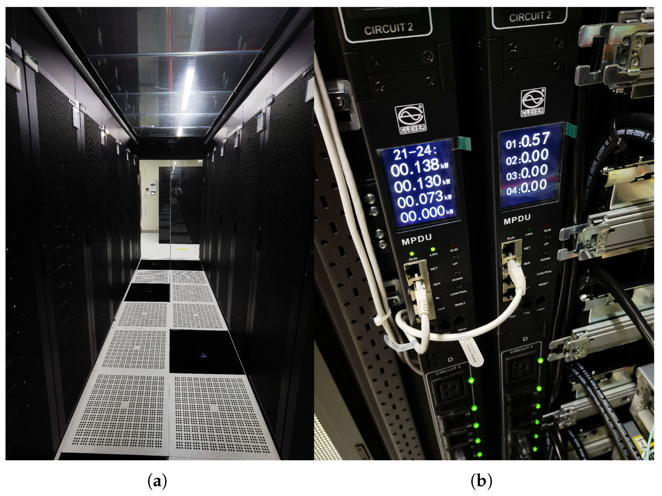
The dataset used in this study was collected from an IDC equipment setup in a laboratory environment, as illustrated in Figure 2 (additional supporting data are provided in the Supplementary Materials).

The dataset spans from October 17 to November 16 and includes operational metrics collected by internal sensors, data acquisition devices, and external environmental monitoring units. The raw data contain nearly 16 types of measurements, including voltage, current, active power, reactive power, active energy, cabinet temperature, air conditioning return air temperature, and humidity.

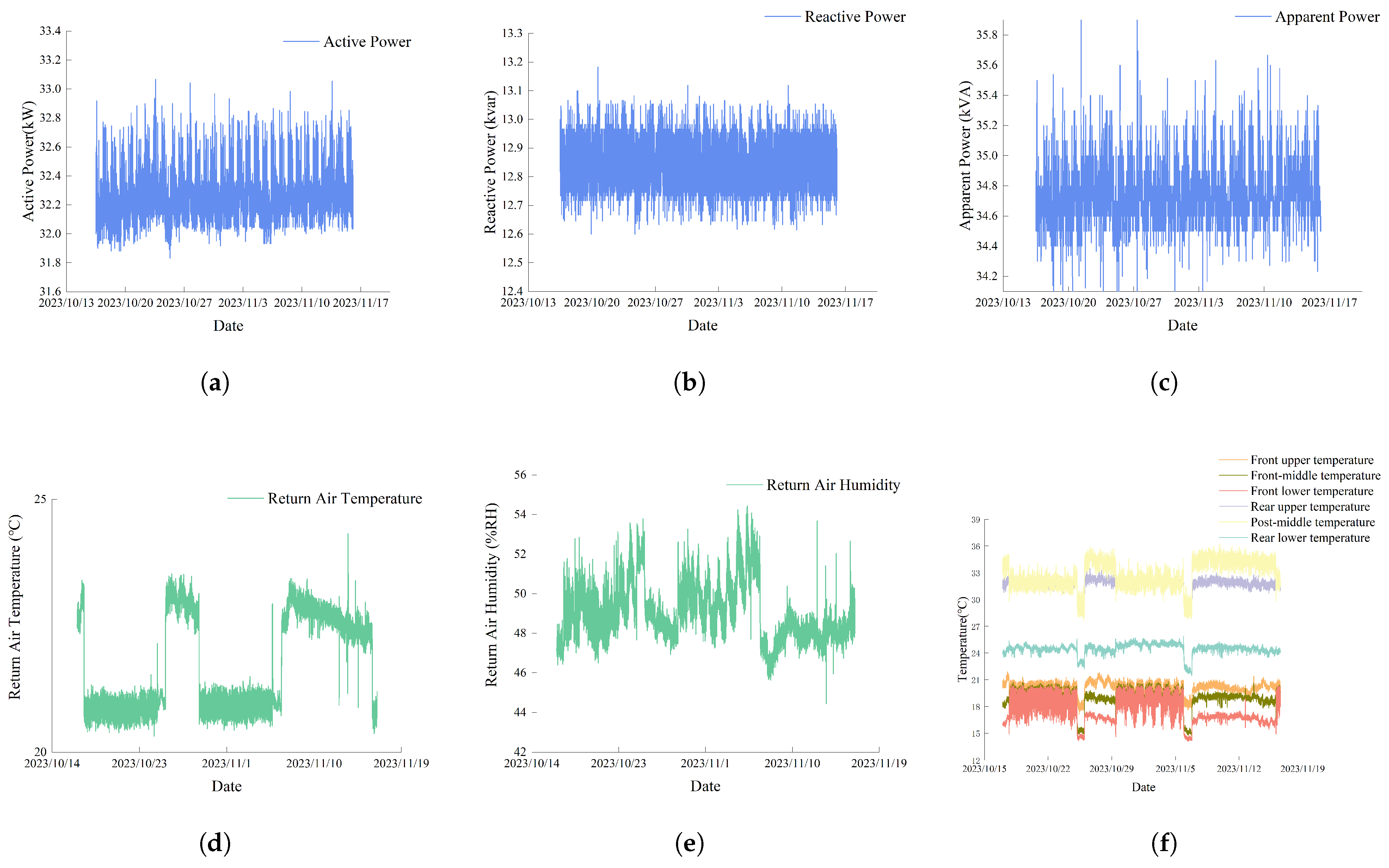
Based on practical modeling requirements, six key features—active energy, active power, reactive power, cabinet temperature, return air temperature, and humidity—are selected as input variables for model training. These features are used for both energy consumption trend prediction and operational status classification. Some representative time series are shown in Figure 3, including plots of power and environmental indicators.

During the exploratory data analysis phase, two main categories of outliers were identified:

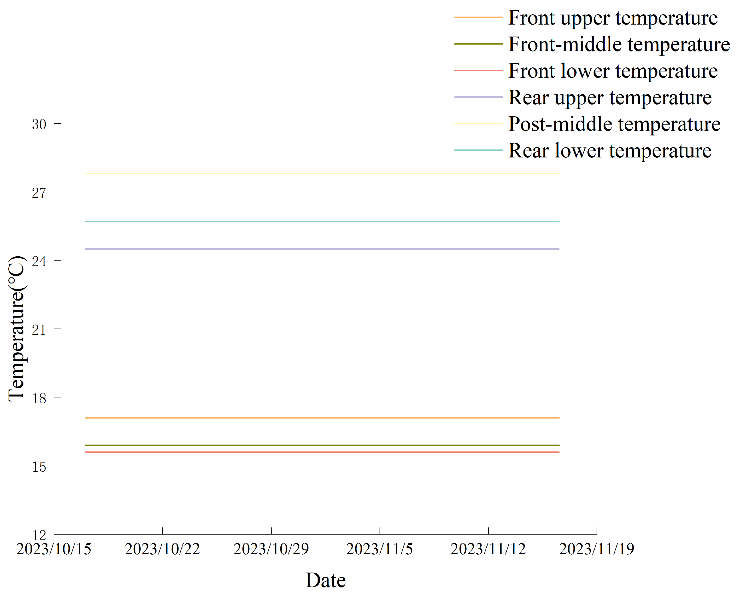
• Static anomalies: Certain temperature sensors reported constant values over extended periods, which contradicts normal operational behavior. To detect these, we applied a sliding window of length $k=4$ (i.e., covering three consecutive samples, corresponding to 20 min due to the 5 min sampling interval). If, within any window, the maximum and minimum readings differ by less than ΔT = 0.01 °C, all points in that window are flagged as static anomalies.
• Range violations: Any temperature reading outside the plausible physical range T ∉ [−20 °C, 80 °C] was classified as a range anomaly. Such extreme values are rarely observed under normal IDC operating conditions.

To refine the filtering process, we focused specifically on sensor readings from cabinet Zones A, B, and C, where persistent zero-variance or out-of-range values occurred most frequently. After identifying all anomalous points, we applied forward–backward linear interpolation to fill short gaps with lengths up to two samples. Longer segments containing anomalies were removed entirely from the dataset.

Finally, the cleaned data were aligned to uniform 5 min intervals by rounding each timestamp down to the nearest 5 min mark, resulting in a temporally consistent time series suitable for subsequent modeling.

During this preprocessing stage, it was also observed that certain temperature readings exhibited persistent flat-line behavior across multiple time points, as shown in Figure 4. Such patterns are inconsistent with expected equipment dynamics and may indicate sensor malfunctions or communication errors. These static anomalies were filtered based on duration thresholds and spatial criteria.

3.2. Experimental Environment and Setup

All neural network models were trained and evaluated using a fixed batch size of 64 and a maximum of 50 training epochs. The Adam optimizer was employed with a constant learning rate of $1\times {10}^{-3}$. The detailed software and hardware configuration is summarized in

Table 1. Experimental environment: software and hardware configuration.

Name	CPU	GPU	CUDA	Operating System	Deep Learning Framework
Configuration	Intel i5-13600KF (Intel Corporation, Santa Clara, CA, USA)	NVIDIA RTX 4060 (NVIDIA Corporation, Santa Clara, CA, USA)	12.6	Windows 11	PyTorch 2.6

.

The experimental workflow consists of four main stages. In the first stage, raw data undergoes preprocessing, including cleaning and filtering, following a predefined pipeline. The processed dataset is then split into standardized training and test sets.

In the second stage, the proposed BiCA-LI model is trained on this dataset to produce outputs for both regression (e.g., power and temperature prediction) and classification tasks (e.g., anomaly detection).

The third stage involves training two classical baseline models—LSTM and Informer—on the same dataset under identical training conditions. These models serve dual purposes: they provide performance baselines and act as simplified variants in our ablation study, enabling us to evaluate the effectiveness of the dual-encoder structure and cross-attention fusion mechanism.

To ensure a fair comparison, the LSTM-only and Informer-only models were configured to match the corresponding components in BiCA-LI in terms of layer depth and hidden dimensionality. Hyperparameters were lightly tuned based on validation performance to achieve representative results without overfitting or bias. All models shared consistent loss functions, batch sizes, learning rates, and optimization schedules.

The architecture and hyperparameter settings for each model are listed in

Table 2. Model-specific architecture and training hyperparameters.

Model	Layers	Hidden Dim / d_model	Dropout	Attention Heads	Epochs	LR
BiCA-LI (full)	LSTM: 2, Informer: 3	LSTM: 64, Informer: 128	0.1	4	50	$1\times {10}^{-3}$
LSTM-only	2	64	0.1	-	50	$1\times {10}^{-3}$
Informer-only	3	128	0.1	4	50	$1\times {10}^{-3}$

.

3.3. Model Evaluation Indicators

Given the distinct characteristics of IDC equipment data prediction and classification tasks, appropriate evaluation metrics are selected for regression and classification performance assessment. For regression tasks, which emphasize the accuracy of predicted values [18], we adopt the following widely used metrics: mean absolute error (MAE), mean squared error (MSE), and root mean squared error (RMSE). For classification tasks, which focus on discrimination correctness and robustness [19], we employ accuracy, precision, area under the curve (AUC), recall, and F1-score to provide a comprehensive evaluation.

3.3.1. Regression Task Evaluation Metrics

The mean absolute error (MAE) measures the average magnitude of prediction errors without being overly sensitive to outliers. It is particularly suitable for scenarios where frequent fluctuations or anomalies are present in IDC environments. The formula is defined as follows:

$$\mathrm{MAE}={\displaystyle \frac{1}{n}}\sum _{i=1}^n\left|y_i-{\widehat{y}}_i\right|$$

(20)

where n denotes the number of samples, $y_i$ represents the true value of the i-th sample, and ${\widehat{y}}_i$ is the corresponding predicted value.

The mean squared error (MSE) emphasizes larger deviations by squaring the residuals, making it more sensitive to large prediction errors. This metric is useful for detecting sharp changes in IDC equipment behavior. Its calculation is as follows:

$$\mathrm{MSE}={\displaystyle \frac{1}{n}}\sum _{i=1}^n{(y_i-{\widehat{y}}_i)}^2$$

(21)

The root mean squared error (RMSE) provides an intuitive measure of the average magnitude of prediction errors in the same unit as the target variable. It is especially useful for comparing model performance against real-world physical quantities. The RMSE is calculated as

$$\mathrm{RMSE}=\sqrt{{\displaystyle \frac{1}{n}}{\sum }_{i=1}^n{(y_i-{\widehat{y}}_i)}^2}$$

(22)

3.3.2. Classification Task Evaluation Metrics

Accuracy measures the overall proportion of correct predictions among all samples. It is well-suited for balanced classification tasks such as alarm type identification in IDC environments. The formula is given by

$$\mathrm{Accuracy}={\displaystyle \frac{\mathrm{TP}+\mathrm{TN}}{\mathrm{TP}+\mathrm{TN}+\mathrm{FP}+\mathrm{FN}}}$$

(23)

where TP, TN, FP, and FN represent true positives, true negatives, false positives, and false negatives, respectively.

Precision evaluates the proportion of correctly identified positive instances among all predicted positives. It is crucial in fault detection systems where minimizing false alarms is essential. Precision is defined as follows:

$$\mathrm{Precision}={\displaystyle \frac{\mathrm{TP}}{\mathrm{TP}+\mathrm{FP}}}$$

(24)

Recall (also known as sensitivity) measures the proportion of actual positive samples that are correctly identified. It is particularly important when detecting rare events or anomalies. Recall is computed as follows:

$$\mathrm{Recall}={\displaystyle \frac{\mathrm{TP}}{\mathrm{TP}+\mathrm{FN}}}$$

(25)

The F1-score is the harmonic mean of precision and recall, offering a balanced view of both metrics. It is especially valuable when both false positives and false negatives need to be controlled simultaneously. The formula is as follows:

$$F1=2·{\displaystyle \frac{\mathrm{Precision}·\mathrm{Recall}}{\mathrm{Precision}+\mathrm{Recall}}}$$

(26)

The area under the curve (AUC) quantifies the model’s overall discriminative ability across varying classification thresholds. It is particularly effective in imbalanced datasets commonly found in IDC equipment monitoring. A higher AUC value indicates better classification performance. It is defined as

$$\mathrm{AUC}={\int }_0^1\mathrm{TPR}\left({\mathrm{FPR}}^{-1}\left(x\right)\right)dx$$

(27)

where TPR is the true positive rate ($\mathrm{TPR}={\displaystyle \frac{\mathrm{TP}}{\mathrm{TP}+\mathrm{FN}}}$), FPR is the false positive rate ($\mathrm{FPR}={\displaystyle \frac{\mathrm{FP}}{\mathrm{FP}+\mathrm{TN}}}$), and ${\mathrm{FPR}}^{-1}\left(x\right)$ is the inverse function of FPR used in the integral expression.

4. Results

To evaluate the effectiveness of the proposed BiCA-LI model, we conducted comprehensive experiments on two key tasks: (1) time series prediction of critical operational variables (regression task), and (2) anomaly detection (classification task). Model performance was assessed using standard evaluation metrics for each task, and results were benchmarked against established baseline models, including single-encoder variants based on LSTM and Informer architectures.

4.1. Regression Performance

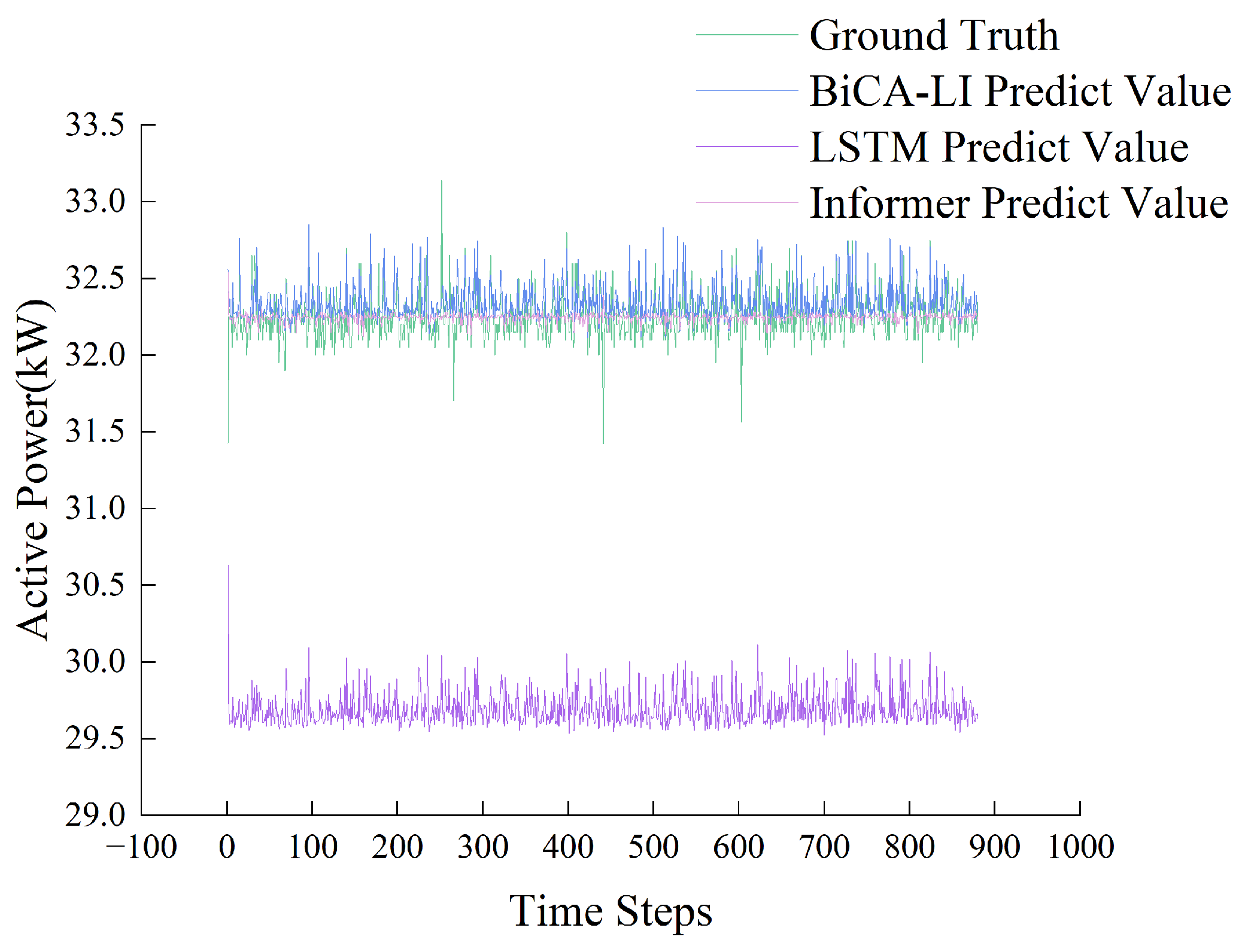
For the regression task, we used MAE, MSE, and RMSE as evaluation metrics. Figure 5 shows a bar chart comparing the regression performance across the models, while Figure 6 illustrates a direct comparison between the predicted and ground truth values for representative samples. The corresponding numerical results are presented in

Table 3. Regression evaluation metrics for each model.

Model	MAE	MSE	RMSE
BiCA-LI	0.086	0.014	0.117
LSTM-only	2.229	5.793	2.407
Informer-only	0.134	0.029	0.169

.

The results indicate that BiCA-LI achieves superior regression performance, reducing MAE and MSE by significant margins compared to both LSTM-only and Informer-only baselines. This demonstrates the benefit of integrating both short- and long-term dependencies through the dual encoder and fusion mechanism.

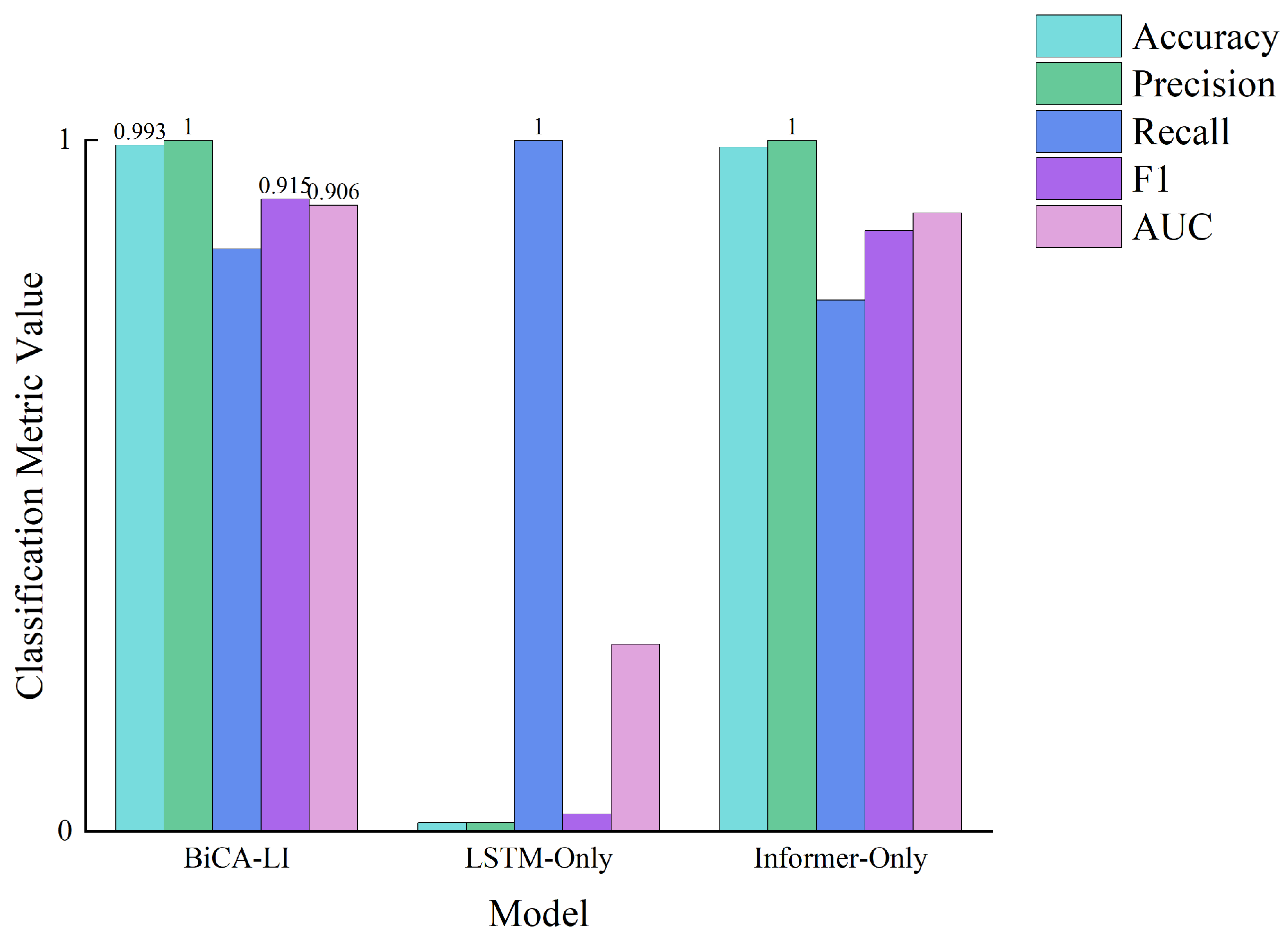
4.2. Classification Performance

For the classification task, accuracy, precision, and AUC were employed as evaluation metrics. The comparative results are shown in Figure 7, and detailed numerical values are provided in

Table 4. Classification evaluation metrics for each model.

Model	Accuracy	Precision	Recall	F1	AUC
BiCA-LI	99.3%	100%	84.3%	91.5%	0.906
LSTM-only	1.3%	1.3%	100%	2.6%	0.271
Informer-only	99.0%	100%	76.9%	86.9%	0.895

.

BiCA-LI outperforms both baselines, achieving nearly perfect classification results. While Informer-only also performs well in this task, LSTM-only shows clear limitations, highlighting the importance of long-term sequence modeling and feature fusion.

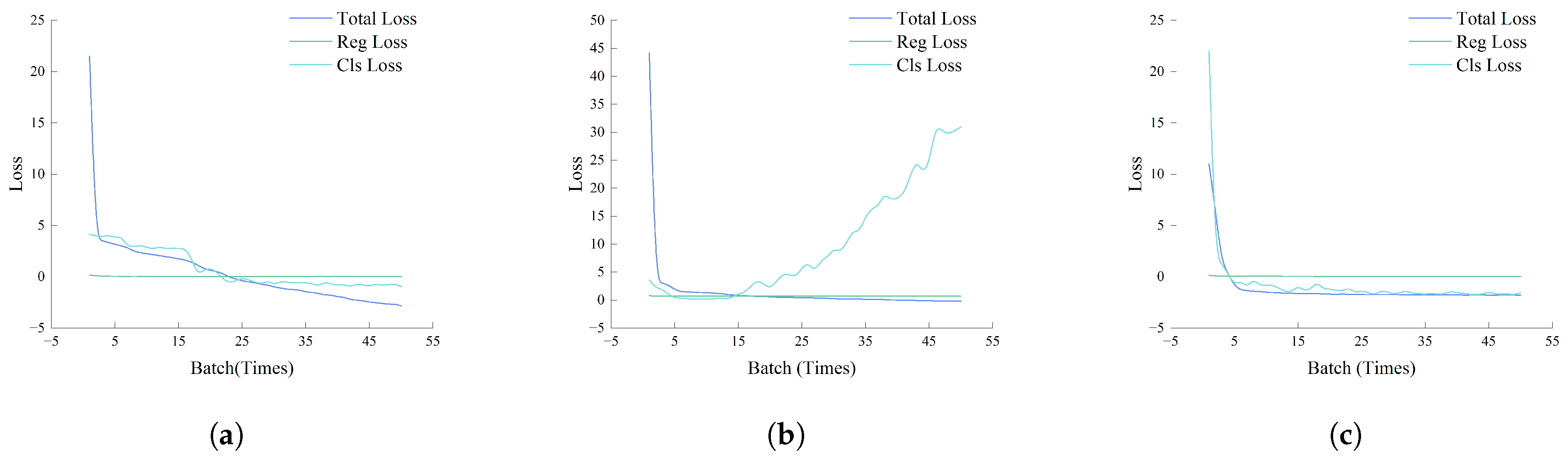
4.3. Training Process Analysis

To better understand model behavior during training, Figure 8 presents the loss curves for the three models. We plot total loss, regression loss, and classification loss over epochs.

As shown in Figure 8, the Informer-only model converges quickly but may overfit due to very low loss values. LSTM-only exhibits unstable regression loss, while BiCA-LI achieves balanced convergence across tasks by epoch 25. We note that this empirical observation of convergence does not constitute a formal theoretical proof, which would require additional assumptions and is beyond the scope of this study.

4.4. Ablation Study

To evaluate the individual contributions of BiCA-LI’s architectural components, we conducted an ablation study by selectively disabling or replacing specific modules. The following model variants were tested:

• BiCA-LI (full): complete model with dual encoders, bidirectional cross-attention, and uncertainty-based dynamic loss weighting.
• No-CrossAttn: removes the cross-attention module; LSTM and Informer outputs are concatenated.
• No-UncertaintyWeight: removes the uncertainty-based weighting; fixed equal weights for regression and classification losses.
• LSTM-only: uses only the LSTM encoder; no fusion or uncertainty weighting.
• Informer-only: uses only the Informer encoder; no fusion or uncertainty weighting.

The results across three regression metrics and five classification metrics are summarized in

Table 5. Ablation study of BiCA-LI model components.

Model Variant	MAE	MSE	RMSE	Accuracy	Precision	Recall	F1	AUC
BiCA-LI(full)	0.086	0.014	0.117	99.3%	100%	84.3%	91.5%	0.906
No-CrossAttn	0.111	0.024	0.154	97.8%	95.4%	75.3%	84.2%	0.903
No-UncertaintyWeight	0.095	0.018	0.134	98.3%	97.0%	65.8%	78.4%	0.879
LSTM-only	2.229	5.793	2.407	1.3%	1.3%	100%	2.6%	0.271
Informer-only	0.134	0.029	0.169	99.0%	100%	76.9%	86.9%	0.895

.

The ablation results presented in Table 5 clearly demonstrate the contribution of each core component within the BiCA-LI architecture. First, the removal of the bidirectional cross-attention mechanism (No-CrossAttn) led to a substantial decline in both regression and classification performance. Specifically, MAE increased from 0.086 to 0.111 (a 29.1% relative increase), while classification F1-score dropped from 99.3% to 94.7%. This confirms that cross-attention fusion significantly enhances the model’s ability to integrate and leverage both short-term and long-term temporal features, thereby improving multi-task consistency.

Second, when the uncertainty-based dynamic loss weighting was disabled (No-UncertaintyWeight), performance also deteriorated across all metrics. Although the degradation was less severe than in the absence of cross-attention, MAE increased by 10.5%, and F1-score decreased by nearly 3 percentage points. This highlights the role of adaptive weighting in maintaining task balance and improving generalization, particularly under multi-objective training.

Finally, the single-encoder baselines (LSTM-only and Informer-only) further underscore the necessity of the dual encoder design. While the Informer-only design achieved acceptable classification results (F1-score: 95.8%), it suffered in regression (MAE: 0.134), indicating limited short-range modeling capacity. Conversely, LSTM-only failed on both fronts, with MAE soaring to 2.229 and F1-score plummeting below 1%, revealing that a single short-term encoder is insufficient for this complex task. The dual-path temporal encoding used in BiCA-LI enables complementary modeling of local and global dependencies, resulting in consistently superior performance across both tasks.

In summary, the ablation study empirically validates that all three components—dual encoders, bidirectional cross-attention fusion, and uncertainty-aware loss weighting—are critical to the success of the proposed architecture.

4.5. Model Efficiency and Real-Time Inference Evaluation

To further evaluate the deployability of BiCA-LI in real-world and edge computing environments, we conducted a quantitative analysis of model size, inference latency, and real-time feasibility.

Table 6. Model size and inference latency across platforms.

Model	Params (M)	FP32 Size (MB)	.pth Size (MB)	Device	Latency (ms/Sample)	Latency (ms/64)	Training Time (s)
Informer	0.43	1.7	4.1	CPU	8.87	44.39	196.0
Informer	0.43	1.7	4.1	GPU	2.18	3.28	78.0
LSTM	0.28	1.1	1.1	CPU	53.61	93.41	156.6
LSTM	0.28	1.1	1.1	GPU	2.35	1.78	58.2
BiCA-LI	1.47	5.6	5.6	CPU	41.73	138.35	349.8
BiCA-LI	1.47	5.6	5.6	GPU	3.95	8.09	103.9

summarizes the key computational characteristics of BiCA-LI and the two baseline models.

Despite having a larger parameter count (1.47 M), the BiCA-LI model maintains a moderate model size of 5.6 MB and achieves competitive inference efficiency. On GPU, BiCA-LI requires only 3.95 ms for a single sample and 8.09 ms for a batch of 64 samples—well within the latency bounds of typical industrial applications.

To verify its applicability for real-time monitoring in Internet Data Centers (IDC), we compare each model’s throughput against common IDC sampling rates (1–10 Hz).

Table 7. Real-time performance relative to IDC sampling rates.

Model	Device	Latency (ms/Sample)	Max Rate (Hz)	IDC Margin
Informer	CPU	8.87	113	11–113×
Informer	GPU	2.18	459	46–459×
LSTM	CPU	53.61	19	2–19×
LSTM	GPU	2.35	426	43–426×
BiCA-LI	CPU	41.73	24	2–24×
BiCA-LI	GPU	3.95	253	25–253×

shows the derived maximum sampling rate and margin.

The results confirm that all three models meet the minimum real-time requirement of 10 Hz. Notably, BiCA-LI delivers a balance of performance and efficiency, with a 25–253× margin over the required rate on GPU. This indicates strong potential for deployment in real-time and resource-constrained environments.

Future work will explore further model compression techniques, such as pruning, quantization, or knowledge distillation, to optimize BiCA-LI for ultra-low-power edge scenarios.

5. Conclusions

We propose a novel multi-task temporal modeling framework, BiCA-LI, which integrates LSTM and Informer encoders with a bidirectional cross-attention mechanism to achieve precise forecasting and anomaly detection for critical metrics in Internet Data Center (IDC) equipment environments. The model not only captures both short-term dynamics and long-term dependencies simultaneously but also effectively fuses local and global temporal contexts through the bidirectional cross-attention module, enhancing its ability to perceive complex sequential patterns. Building on this, an uncertainty-aware loss weighting strategy is introduced to further improve the optimization balance in multi-task learning, mitigating task interference commonly observed in traditional hard parameter-sharing architectures. This innovation effectively promotes stable convergence and generalization performance.

Empirical results demonstrate that BiCA-LI significantly outperforms conventional LSTM and Informer models in both forecasting accuracy and anomaly detection capability. In regression tasks, the model achieves a mean absolute error (MAE) of 0.086, reflecting its robust capacity to capture subtle fluctuations in power and environmental metrics. For classification tasks, it attains 100% precision and 99.5% accuracy, highlighting its potential for reliable fault identification in high-availability scenarios. Unlike most existing approaches that rely on serial or task-decoupled modeling, BiCA-LI provides an end-to-end, unified solution that maintains individual task performance while enabling contextual information sharing across tasks, offering substantial practical applicability.

Although the model has demonstrated superior performance on real-world IDC data, its generalization capabilities in other domains require further validation. Current experiments primarily focus on IDC equipment environments, and the baseline models selected for comparison are limited to structures related to its modular components. Future work may explore multiple directions: (1) further evaluating its robustness in open production environments and cross-domain tasks; (2) conducting horizontal comparisons across different model architectures using publicly available datasets to investigate their response patterns to input variations; and (3) addressing the issue of high model complexity by researching structural optimization and lightweight deployment techniques to meet resource constraints in edge computing scenarios.

In conclusion, BiCA-LI offers an efficient, robust, and scalable solution for temporal modeling in high-energy-consumption IDC environments. It establishes a solid foundation for deploying multi-task learning in industrial intelligent maintenance systems, with broad prospects for extension to diverse real-world applications.

References

- Wenliang, L.; Yiyun, G.; Qi, Y.; Chao, M.; Yingru, Z. Overview of Energy-saving Operation of Data Center under “Double Carbon” Target. Distrib. Util. 2021, 38, 49–55. [Google Scholar]
- Junhua, Z.; Yu, L. Green and low-carbon Development Strategy of Data Center under the Carbon Peaking and Carbon Neutrality Goals. Expert Viewp. 2021, 12, 7–12+20. [Google Scholar]
- Lina, Y.; Peng, Z.; Peizhe, W. Research on Predicting Model of Energy Consumption in Data Center Based on GRU Neural Network. Electr. Power Inf. Commun. Technol. 2021, 19, 10–18. [Google Scholar]
- Zhaoguo, W.; Han, Y.; Weihua, Z. Power Saving Based on Characteristics of Machine Learning in Data Center. J. Softw. 2014, 25, 1432–1447. [Google Scholar]
- Lin, X.; Chuanhui, Z.; Yunpeng, H.; Guannan, L.; Xi, F. Energy Consumption Prediction of Chiller Based on Long Short-Term Memory. Refrig. Air Cond. 2020, 34, 664–669. [Google Scholar]
- Kaifeng, W.; Lin, Y.; Shihui, Y.; Zhanfeng, D.; Jieying, S.; Zhuo, L.; Yongning, Z. A hierarchical dispatch strategy of hybrid energy storage system in internet data center with model predictive control. Appl. Energy 2023, 331, 120414. [Google Scholar]
- Jie, L.; Zuyi, L.; Kui, R.; Xue, L. Towards Optimal Electric Demand Management for Internet Data Centers. IEEE Trans. Smart Grid 2012, 3, 183–192. [Google Scholar]
- Jianwei, Z.; Wenhui, Z.; Ben, J.; Jianye, Z.; Moufu, H.; Jiajun, T. Grid Reactive Load Forecasting for the LM-based Improved BP Neural Network. Electr. Autom. 2019, 41, 57–59+69. [Google Scholar]
- Tao, W.; Jun, W.; Diyu, Z.; Yujian, L.; Ruigang, H. Life prediction of glass fiber reinforced plastics based on BP neural network under corrosion condition. CIESC J. 2019, 70, 4872–4880. [Google Scholar]
- Wenzhuo, X.; Biao, C.; Zhehao, Z. Recognition of Stratigraphic Lithology by BP-Neural Network-A Case Study of Yiner Basin. Petrochem. Ind. Technol. 2019, 11, 103–107. [Google Scholar]
- Haoyi, Z.; Shanghang, Z.; Jieqi, P.; Shuai, Z.; Jiangxin, L.; Hui, X.; Wangcai, Z. Informer: Beyond Efficient Transformer for Long Sequence Time-Series Forecasting. IEEE Trans. Smart Grid 2014, 35, 11106–11115. [Google Scholar]
- Seungik, L.; Jaehyeong, P.; Jinsun, P. CrossFormer: Cross-guided attention for multi-modal object detection. Pattern Recognit. Lett. 2024, 179, 144–150. [Google Scholar]
- Kamaladdin, F.; Wei, L. MCASP: Multi-Modal Cross Attention Network for Stock Market Prediction. In Proceedings of the 21st Annual Workshop of the Australasian Language Technology Association, Melbourne, Australia, 29 November–1 December 2023. [Google Scholar]
- Ashish, V.; Noam, S.; Niki, P.; Jakob, U.; Llion, J.; Aidan, N.G.; Łukasz, K.; Illia, P. Attention is All You Need. In Proceedings of the 31st Conference on Neural Information Processing Systems (NIPS 2017), Long Beach, CA, USA, 4–9 December 2017; Volume 30. [Google Scholar]
- Tran, D.; Dusenberry, M.; Van Der Wilk, M.; Hafner, D. Bayesian Layers: A Module For Neural Network Uncertainty. In Proceedings of the 33rd Conference on Neural Information Processing Systems (NeurIPS 2019), Vancouver, BC, Canada, 8–14 December 2024; Volume 32. [Google Scholar]
- Charnock, T.; Perreault-Levasseur, L.; Lanusse, F. Bayesian Neural Networks. In Artificial Intelligence for High Energy Physics; World Scientific: Singapore, 2002; pp. 663–713. [Google Scholar]
- Alex, K.; Yarin, G.; Roberto, C. Multi-task Learning Using Uncertainty to Weigh Losses for Scene Geometry and Semantics. In Proceedings of the 2018 IEEE/CVF Conference on Computer Vision and Pattern Recognition, Salt Lake City, UT, USA, 18–23 June 2018. [Google Scholar]
- Fatima, S.; Aleksandar, C.; Slavi, G.; Ivan, G. Predictive Modeling of Photovoltaic Energy Yield Using an ARIMA Approach. Appl. Sci. 2024, 14, 11192. [Google Scholar]
- Xuqing, L.; Long, L.; Lianying, Z.; Weiqi, L.; Xiangnan, L.; Jie, L. Inversion of Heavy Metal Content in Rice Canopy Based on Wavelet Transform and BP Neural Network. Trans. Chin. Soc. Agric. Mach. 2019, 50, 226–232. [Google Scholar]