Abstract
Traditional permanent-magnet synchronous motor (PMSM) models assume constant inductance parameters in the dq frame, attributing torque ripple solely to local non-sinusoidal disturbances while neglecting nonlinear effects like iron saturation, flux linkage spatial harmonics, and inter-axis mutual coupling. These simplifications limit such models to predicting average torque but fail to capture harmonic components. To overcome these limitations, this study develops a nonlinear PMSM model using differential inductance theory and constructs a physics-informed neural network (PINN) surrogate trained on finite-element data. The proposed hybrid framework demonstrates high-fidelity torque prediction, validated against finite-element simulations, and provides insights into harmonic generation mechanisms under saturation and spatial field distortions.
1. Introduction
Permanent magnet synchronous motors (PMSMs) offer advantages over traditional asynchronous motors, such as high efficiency, high power density, fast response, and low noise. These features enable electric vehicles (EVs) to achieve better acceleration performance, longer driving range, and improved control accuracy, making PMSMs widely used in EV drivetrain systems [1]. Additionally, PMSMs can function as energy storage components in lithium-ion battery AC heating systems [2,3].
The construction of traditional PMSM models relies on parameters including stator equivalent resistance , dq-axis equivalent inductances , , and permanent magnet flux linkage . By adopting the synchronous rotating coordinate system, the control complexity of alternating quantities in the motor is effectively simplified; meanwhile, the double-reaction theory addresses inductance fluctuations caused by uneven air gaps in salient-pole motors, forming a simplified constant-parameter PMSM model with concise formulations. However, to facilitate model development, this approach simplifies and linearizes the real physical model of PMSMs under four key assumptions:
- Magnetic saturation effects in the core magnetic circuit are neglected.
- The magnetic potential in the air-gap field and the back-EMF generated by permanent magnets contain no harmonics.
- The rotor has no damper windings, and permanent magnets exhibit no damping effects.
- Hysteresis and eddy current losses in the motor, as well as magnetic circuit nonlinearity, are not considered.
These assumptions deviate from the motor’s actual operating conditions, especially in vehicle drivetrain systems where stator and rotor cores often operate in a high magnetic saturation state to achieve high power density [4]. Under load, the air-gap magnetic field of the motor rarely maintains an ideal sinusoidal distribution [5]. Therefore, to accurately simulate the voltage–current excitation response characteristics at specific operating points, it is necessary to comprehensively consider physical phenomena affecting parameter characteristics, such as magnetic saturation [6,7], cross-coupling effects [8,9], rotor magnetic field harmonics, and loss-induced temperature rise.
The relative permeability of motor ferromagnetic materials exhibits a nonlinear relationship with magnetic field strength : when is low, the relative permeability of the core is high; once exceeds a critical value, the relative permeability decreases rapidly, making core reluctance effects non-negligible. As the degree of magnetic saturation increases, nonlinear reluctance differences at different spatial positions in the motor significantly exacerbate the non-sinusoidal distribution of the air-gap field, causing obvious changes in the dq-axis inductance parameters under different stator current excitations , [10,11]. Furthermore, core magnetic saturation induces cross-coupling phenomena, generating mutual inductances , between orthogonal dq-axis windings, and the magnitude of these mutual inductances can approach that of the dq-axis self-inductances under deep saturation [5,12].
Many scholars have studied the nonlinear relationships of physical quantities in PMSMs. Weidenholzer et al. [13] abandon the explicit calculation of absolute inductances in PMSM modeling and instead directly construct a stator flux linkage model. This method comprehensively considers magnetic saturation, cross-coupling, and rotor magnetic field harmonic effects, defining the stator flux linkage as a three-dimensional function of dq-axis currents and rotor angle. Flux linkage MAP tables are generated through finite element analysis (FEA) combined with radial basis function (RBF) interpolation, and a nonlinear model is then constructed using look-up table modules. This modeling approach replaces complex functional operations with discretization processing, significantly reducing computational load and improving real-time performance. Rahman et al. [14] proposed an advanced modeling method for interior synchronous motors, developing a dynamic motor model that considers magnetic saturation effects and the rotational-angle dependence of electrical, magnetic, and mechanical quantities, which can be integrated into multidisciplinary system simulations. Based on RBF interpolation technology, this model is constructed using a set of magnetic field finite element method (FEM) solution data. The proposed motor model can simulate arbitrary time-stepping operating conditions, such as field-weakening control research, sensorless motor control algorithm analysis, or short-circuit characteristic simulation, without the need for real-time magnetic field FEA during operation.
High-precision PMSM models depend not only on the accuracy of parameters such as flux linkage and inductance but also require the establishment of new motor mathematical models to achieve more accurate torque prediction. Nakao and Akatsu [15] developed a Global Linearization Model (GLM), assuming linearization within the PMSM’s operating range and considering the effects of non-sinusoidal distortion in inductances and flux linkage, as well as magnetic energy fluctuations under open-circuit conditions, on torque. However, the linearity assumption fails in the saturation region, limiting the model’s application scope. Lee et al. [16] used the frozen permeability method (FPM) to establish a torque model and analyzed the torque of PMSMs under steady-state current excitation. However, since the model still uses apparent inductances, the torque model only includes derivatives of flux linkage and magnetic energy, unable to account for torque ripple under non-steady-state excitation. Rezaee-Alam, F. [17] proposed a new algorithm combining the virtual work principle and the FPM, enabling appropriate on-load torque ripple calculation in both linear and nonlinear scenarios. Wang et al. [18] proposed a nonlinear PMSM model based on differential inductance, establishing differential equations for flux linkage, magnetic energy, and torque with current and electrical angle as independent variables. By using FEA to obtain parameters such as motor differential inductance, flux linkage, and magnetic energy, and calculating torque through the introduction of saturated flux linkage differences, this approach achieves accurate prediction of torque ripple. However, the prediction accuracy of this method depends on the fine grid division of FEA operating points, and the local linearization assumption under non-steady-state excitation can introduce errors, reducing prediction accuracy.
In recent years, approaches synergistically integrating physics-informed knowledge with data have gained significant traction for control and modeling in power electronics and motor drives. This trend highlights the potential of physics-informed neural networks (PINNs) to overcome challenges in electromagnetic modeling, such as the precise calculation of torque in permanent magnet synchronous motors (PMSMs). Conventional methods like FEA, while accurate, suffer from the absence of explicit functional relationships and significant computational expense.
PINNs emerge as a promising solution, grounded in the universal approximation theorem. Their core methodology involves embedding the governing physical equations and boundary conditions directly into the neural network’s loss function. This ensures the back-propagation process inherently respects the underlying physics, enabling the network to iteratively approximate the system’s true physical structure through training [19,20,21]. Crucially, PINNs bypass the need for complex discretization schemes and numerical algorithms typical of traditional PDE solvers. Instead, they leverage automatic differentiation (AD) techniques during backpropagation to accurately characterize differential operators. This AD approach offers robustness against noisy data, a distinct advantage over numerical differentiation methods like finite differences. Furthermore, the inherently meshless nature of PINNs eliminates the tedious process of mesh generation, effectively transforming the complexity of the physical problem into a focused network optimization task. The efficacy of this approach is demonstrated in relevant applications, particularly for PMSM modeling. Xia et al. [22] successfully applied PINNs for parameter identification in PMSMs. Their work constructed a high-fidelity motor model capable of capturing critical nonlinear effects like magnetic saturation and cross-coupling. This was achieved by utilizing polynomial fitting to characterize dq-axis flux–current relationships while embedding the fundamental motor voltage equations into the PINN’s loss function. This physics-constrained framework enabled robust parameter optimization, subsequently validated through both simulation and experiment. The principle of embedding physical knowledge into learning frameworks is also evident in other power electronics domains, as seen in Zeng et al.’s [23] work on optimizing DAB converters using a physics-informed deep transfer reinforcement learning method.
However, as demonstrated by Cuomo, S. et al. [24], soft constraints indirectly impose boundary conditions or physical laws through penalty terms in the loss function. They cannot guarantee strict satisfaction of boundary conditions, their weighting relies on subjective tuning (prone to imbalance between competing constraints during optimization), are susceptible to local minima in high-dimensional or nonlinear problems, lack strict theoretical convergence guarantees, and exhibit insufficient robustness to noisy data and complex geometric scenarios.
This paper is organized as follows: Section 2 derives the mathematical model of a PMSM in both ABC and dq0 reference frames based on differential inductance and conducts angular frequency-domain analysis. Section 3 presents the methodology for constructing physical constraints specific to PMSMs and details the corresponding PINN architecture. Section 4 establishes a PINN surrogate model using a finite element model of a 4-pole 48-slot interior PMSM, validating the accuracy of its torque calculations through comparative analysis with alternative approaches.
2. The Nonlinear PMSM Electromagnetic Model Based on Differential Inductance
To address the limitations inherent in conventional linear models—particularly the assumptions of constant inductance, negligible magnetic saturation, and sinusoidal flux linkage distributions—this study develops a nonlinear modeling framework grounded in differential inductance theory. In saturated electromagnetic systems, the differential inductance physically represents the local sensitivity of the flux linkage–current relationship under nonlinear operating conditions. For polyphase systems, this concept generalizes to the Jacobian matrix of the flux linkage vector with respect to the current vector, expressed as:
Since the differential relations required for the torque model are provided only by differential inductance, the inductances appearing below are differential without explanation.
2.1. PMSM Equations in the ABC Frame
When the electrical angle is constant, the inductance, magnetic energy, and flux linkage of the motor are all functions of current only. Following the definition of differential inductance, the armature flux linkage in the ABC frame can be expressed as:
In (2), and denote the differential inductance matrix and current vector in the ABC frame, respectively. When there is no current excitation, the flux linkage is provided only by the permanent magnet, so the initial condition for the integration of the above equation is . When incorporating the permanent magnet flux linkage , the total flux linkage of the motor in the ABC stationary reference frame can be expressed as:
Consider the conservation of energy in the motor system in the steady state. Excluding iron losses and high-frequency eddy current effects, the electrical energy input to the motor system is fully converted into mechanical energy and magnetic energy :
Among them:
where is the mechanical angle (, is the number of pole pairs). In this system, all physical quantities in steady-state conditions are related only to the excitation and the electrical angle , both and can be considered independent state variables. It follows that the system energies may be expressed as total differential forms with respect to variations in and :
Substituting (6)–(8) into (4) and collapsing gives:
Since the above equation holds for any and while and are independent variables, the coefficients before and must be constant to zero. Therefore, the torque equation can be obtained from the term:
The magnetic energy equation can be obtained by making the coefficient of the term of (9) equal to zero:
Under no-load conditions, the motor’s armature contributes no magnetic field energy, with the system’s entire magnetic field energy originating exclusively from the permanent magnets. When the motor is loaded, variations in magnetic field energy arise solely from current excitation. Consequently, the aforementioned energy relationship can be expressed in integral form, where the initial condition represents the permanent magnets’ magnetic field energy:
For further analysis, define the magnetic co-energy:
Thus, the torque Equation (9) can be simplified as:
can be decomposed as follows:
Following the definitions and formulations of all motor physical quantities, the subsequent analysis delves into the motor’s mathematical model from a field-theoretic perspective. Since the differential inductance is the Jacobi matrix of the flux linkage , and also is a symmetric array, it follows that has zero curl in ABC frame:
defines a curl-free field, then there must exist a potential function for the field such that:
This can be proved according to (2) (15):
The preceding analysis demonstrates that the magnetic co-energy serves as a scalar potential function for the curl-free component of the flux linkage field under specified initial conditions. Since the permanent magnet flux linkage and initial rotor position are independent of stator current excitation and uniquely determine the integration constants, the total co-energy can be decoupled into a linear current-dependent term and a permanent magnet contribution. Consequently, Equation (18) is reformulated as follows:
2.2. PMSM Equations in the dq0 Frame
Under magnetic saturation and dq-axis cross-coupling effects, the mathematical model in the dq0 reference frame transforms AC quantities into DC quantities. However, decoupling of the inductance matrix becomes unattainable under these conditions. Define the dq0-frame variables as follows:
where is the coordinate transformation matrix from ABC to dq0:
Its inverse matrix is given by:
Substituting (20) into (2) yields the equation for the flux linkage equation in dq0 frame:
After transformation, is an asymmetric matrix. Let:
() is the metric tensor, ensuring that the length of vectors remains invariant under coordinate transformations. After the transformation, is still a real symmetric array. Thus, (23) can be rewritten as:
Substituting (20) into (13) yields the magnetic energy equation in dq0 frame:
Combining (10), (25) and (26), the torque equation in the dq0 frame can be derived:
The field equation becomes:
2.3. PMSM Angular Frequency Domain Analysis
The torque Equation (27) contains partial derivative terms and . When the current excitation is a periodic signal on , all the flux linkages, inductances, magnetic energies, and magnetic co-energies are likewise periodic signals on , i.e., in the solution domain , , , , all satisfy the periodic boundary conditions:
Thus, a Fourier series expansion can be performed for the above physical quantities:
where and denote the cosine term Fourier coefficients and sinusoidal term Fourier coefficients, respectively, with the subscript (ind, f, e, coe) represents inductance, armature flux linkage, armature magnetic energy, and armature magnetic co-energy corresponding to the Fourier coefficients, and the superscript denoting the order of the Fourier coefficients. In the dq0 model. Since and are independent variables, based on the uniqueness of the Fourier series and the linear nature of differentiation, combining with (30), the following relationship can be obtained:
The above two sets of relational equations show that the differential relationship between the Fourier coefficients of each physical quantity of the PMSM satisfies the same differential relationship with the original physical quantities, which establishes the mathematical model of the PMSM in the angular frequency domain. According to the above two sets of relations, the partial derivative term about in the equation can be solved conveniently, which creates the foundation for the angular frequency domain analysis of torque ripple.
3. Nonlinear Electromagnetic Modeling of PMSM
The nonlinear PMSM electromagnetic model based on differential inductance is applicable not only to steady-state excitation (SE) conditions where is a constant value, but also to unsteady-state excitation (USE) conditions. (27) shows that accurate prediction of PMSM torque requires characterizing the distributions of inductance, flux linkage, and magnetic energy as functions of electrical angle; for each specified current operating point, these distributions can be evaluated via finite element analysis (FEA). However, in real motor drive applications, is not a constant quantity, and the PMSM generally operates at USE conditions. Since and are generated only by the permanent magnets, and are consistent for any current operating point, it is only necessary to solve for the armature flux linkage and armature magnetic energy for the USE conditions at the non-FEA operating point. Depending on the solution method, there are the Global Linearization Model (GLM) and the optimal linear approximation model (OLAM).
3.1. The Global Linearization Model (GLM)
The inductance in the GLM does not vary with current excitation, then and can be calculated by the following equation:
This model aligns with the classical linear framework that accounts for spatially non-sinusoidal distributions of flux linkage, exhibiting consistent expressions for flux linkage and magnetic energy. Figure 1 depicts the variation in flux linkage and magnetic energy with in the GLM algorithm [15].
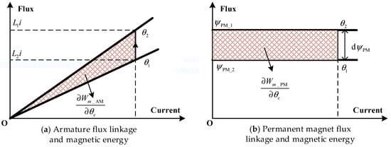
Figure 1.
Relationship between flux linkage, magnetic energy and electrical angle in the GLM. The shaded area represents the variation in magnetic energy induced by changes in electrical angle.
Consequently, GLM is applicable for analyzing torque ripple arising from spatial parameter variations. However, the model does not incorporate the dependence of inductance on excitation levels, leading to increased inaccuracies in saturation regions and limiting its effectiveness in high-precision torque ripple analyses.
3.2. The Optimal Linear Approximation Model (OLAM)
OLAM regards the harmonics in the periodic excitation current as small-signal components , and the flux linkage increment can be obtained by using the tangent-plane function and the differential inductance can be calculated in the approximate linear region by using the differential inductance in the light of the characteristics of the linear electromagnetic structure [25]. Figure 2 shows the locally linearized flux linkage surface. The differential magnetic energy can be calculated in the approximate linear region, and then the localized linearized flux linkage and magnetic energy model containing the differential part can be built at each non-FEA working operating point. According to the flux linkage Equation (25) and magnetic energy Equation (26) the and in the model can be computed by the following equation [14]:
where , the superscript FEA stands for the value of each physical quantity taking the value at the FEA operating point near the USE operating point. When , the model becomes an exact representation of the nonlinear mathematical model, which not only includes spatially non-sinusoidal distributions of the inductance and the flux linkage, but at the same time embodies the saturation characteristics of the magnetic circuit in terms of the differential inductance. However, when the current excitation deviates from the known operating point, increases, the local linearization is no longer valid and the model error increases. In essence, the traditional interpolation method realizes function fitting by selecting the basis function, and the differential properties of the resulting fitted function are only related to the basis function, so it is difficult to realize the fitting of complex field features. Limited by the FEA points, the above method is difficult to realize the approximation of higher-order derivatives and partial derivatives, and it is not possible to further increase the constraints to improve the numerical computation accuracy, which also brings difficulties for the subsequent adoption of the optimization method of gradient descent.
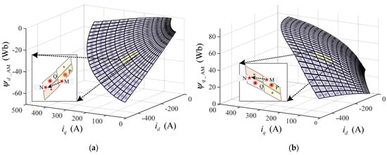
Figure 2.
Armature dq flux linkage surface in the OLAM method. (a) d-axis armature flux linkage; (b) q-axis armature flux linkage. Points P and Q denote FEA-sampled current points, while points M and N denote calculated excitation current points. The nonlinear relationship between flux linkage and current is treated as a differentiable manifold, and tangent planes provide an optimal first-order approximation of this surface.
3.3. The PINN Surrogate Model Based on Physical Priors of PMSM
Since the differential inductance of the PMSM is unknown, the FEA dataset needs to be used to provide the output constraints. In this paper, the flux linkage is chosen as the output of the network. The flux linkage is a quadratic function on the scalar which is dimensionally reduced by Fourier series decomposition to and a series of ternary functions, and the Fourier coefficients are independent of each other, so PINNs can be built separately, which can realize the parallel training and computation while reducing the number of inputs and guaranteeing the characteristics of the frequency domain. Let , corresponding to the PINN input-output functions are, respectively, , , then the network predicted values , , respectively:
Consider the structure of any network , each consisting of an input, a fully connected layer and a physical layer. The inputs of the network are:
The forward propagation expression for the fully connected layer is:
where the superscript denotes the th layer, is the number of hidden layers, , , , are the outputs, activation values, weight matrices, and bias vectors of the th layer, and is the activation function. The fully connected layer is connected to the physical layer. The role of the physical layer is to embed the will physical features of the object into the network by means of hard constraints or loss functions. Take the cosine term Fourier coefficients as an example. The following constraints exist for the PMSM system:
- Constraint 1: has zero curl:
- Constraint 2: and initial conditions are zero:
Hard constraints can be constructed based on the above physical information. Assuming that the number of neurons in the first hidden layer of the fully connected layer is 6, construct:
is a real symmetric matrix consisting of the 6 activation values of the th hidden layer. Let:
is the predicted value of the sum of . (41) makes a quadratic function of . When is equal to , both the function value and the gradient value of are zero. Further, it is possible to make:
Such that satisfies the initial condition of zero (Condition 1) and as the gradient of the scalar, also satisfies the curl to zero (Condition 2). The above equation can be realized in a computer by Pytorch automatic differentiation [26].
Since flux linkages are chosen as training samples, a loss function can be defined:
where is the number of samples and the superscript denotes the predicted or sample value corresponding to the th sample of the th order Fourier coefficient. The loss function is optimized by error back propagation when , , and . In addition, the predicted values of the Fourier coefficients of the inductance can be further derived by automatic differentiation:
The structure of is shown in Figure 3. Different from the classical PINN which adds the physical equation loss term directly into the loss function, the above network structure firstly satisfies the periodic boundary conditions between the network output and input by Fourier series decomposition; then the network automatically satisfies the initial conditions and field equations of each physical quantity by constructing the hard constraints of the curl and the hard constraints of the initial conditions, which embeds the differential features of the motor in the network, to The problem of inconsistent convergence direction of physical and data loss terms is avoided. Finally, the loss function is established using FEA sample data to realize the optimization of network parameters, which reflects the idea of PINN physical information and data fusion driven.
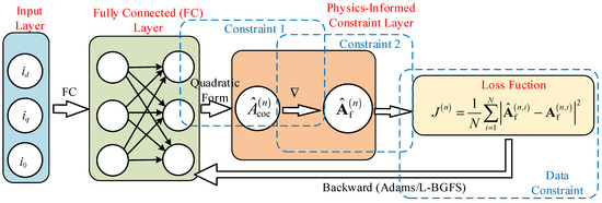
Figure 3.
Network architecture of the PINN-based nonlinear model for a permanent-magnet synchronous motor.
4. Examples of PINN Surrogate Modeling
In order to improve the calculation accuracy, this paper uses Ansys Maxwell 2D transient field solver to complete the FEA calculation and extract the sample data, and then builds and trains the PINN based on the Pytorch platform (https://pytorch.org/) to obtain the PMSM Surrogate model. The model realizes the prediction of PMSM torque and other parameters under SE and USE conditions. The workflow is shown in Figure 4.
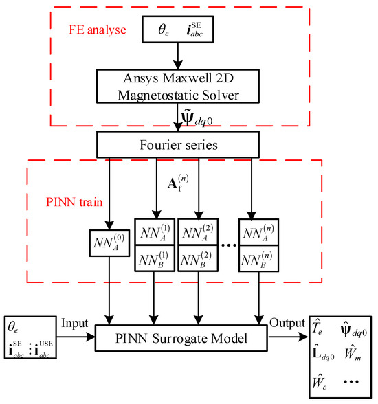
Figure 4.
The workflow of PINN modeling.
4.1. FEA Parameter Extraction
In this paper, the motor is simulated using Maxwell 16.0. The 1/8 finite element model of the motor is shown in Figure 5: The key parameters of the PMSM are listed in Table 1.
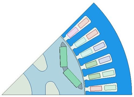
Figure 5.
The finite element model of a 1/8 segment of an interior PMSM.

Table 1.
Key parameters and materials of the PMSM.
4.2. PINN Training
Build and train a neural network based on the Pytorch platform. The DeepXDE library [27] is used by the PINN to compute the Jacobian matrix. According to the analysis in Section 2, for any flux linkage sample Fourier coefficients, a single PINN can be built so that the physical relationship between network inputs and outputs satisfies the physical relationship. The network hyperparameters are designed according to the structure of
Table 2.
Hyperparameters of PINN.
4.3. Analysis of PINN Modeling Results
Figure 6 shows the loss function curves of the Fourier coefficients of the flux linkage for the sine and cosine terms, respectively. The results show that for the 0th-, 6th-, 18th-, and 24th-order Fourier coefficients of , the PINN can converge effectively within 4000 epochs. As the higher order of the Fourier coefficients, the more complex the chain-current relationship is, the lower-order coefficients are fitted best, among which the 0th-order coefficients reflect the DC component and average torque of the armature flux linkage , and the minimum mean square error reaches at all current operating points. The surfaces with 18th- and 24th-order coefficients are very complex, but PINN can still achieve satisfactory results, and the minimum mean square error can reach for all of them.
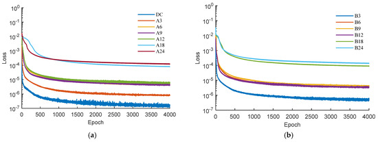
Figure 6.
Training loss curves of the PINN. (a) Cosine term loss; (b) Sine term loss. DC, A6, B6, … denote the loss contributions associated with the , , …, respectively.
The fitting performance of the PINN model for flux linkage is exemplified by the Fourier cosine coefficients, as illustrated in Figure 7, where the continuous surfaces represent PINN-generated results and solid red dots denote FEA sample points. The results demonstrate that the PINN framework achieves high-fidelity reconstruction of flux linkage harmonics across all orders while simultaneously satisfying both numerical agreement with FEA benchmarks and rigorous physical constraints—including curl-free field conditions and specified initial/boundary requirements.
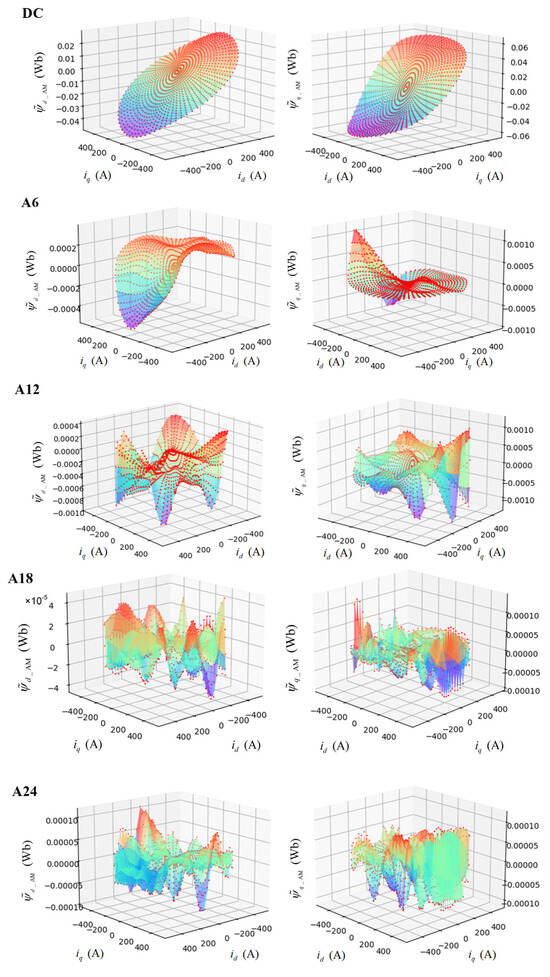
Figure 7.
Fitting Fourier coefficients of armature flux linkage by PINN.
The PINN provides a continuously differentiable model for the PMSM, enabling systematic analysis of their electromagnetic field characteristics. As shown in Figure 8, the Fourier coefficient distribution of the armature magnetic co-energy is visualized alongside the flux linkage vector coefficients (indicated by red arrows). Notably, the flux linkage Fourier coefficient vectors remain perpendicular to the armature co-energy contour lines at all positions, numerically confirming the gradient relationship defined in (42). With increasing harmonic orders, both the armature co-energy and flux linkage distributions exhibit heightened spatial complexity, particularly in saturation-governed weak magnetic regions where localized field variations intensify. These nonlinear saturation effects manifest as sharp transitions in physical quantities and non-orthogonal harmonic interactions, demonstrating the intrinsic nonlinear behavior of PMSM under high saturation conditions.
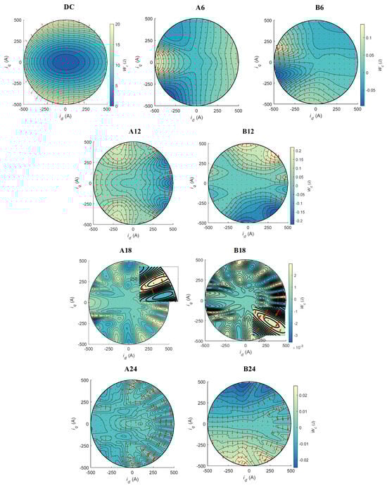
Figure 8.
Distribution of the Fourier coefficients of armature flux linkage and magnetic co-energy over the dq-axis current plane. The boundary denotes the current-limit circle. At every point, the armature flux linkage vector (red arrows in the figure) is perpendicular to the co-energy contour lines.
4.4. PMSM Torque Calculation Based on PINN Modeling
In order to verify the validity of the PMSM nonlinear mathematical model and the PINN Surrogate model, the torque calculations are performed under SE conditions and USE conditions, respectively, and compared with the FEA data and the OLAM results in order to verify the superiority of the PINN model. Theoretically, the farther the selected calculation operating point deviates from the FEA operating point, the larger the error between the parameter surfaces of the OLAM and the PINN model and the actual parameters are. In this paper, the typical field weakening operating point (, ) and the operating point (, ) are computed and verified, where is the current amplitude and is the angle of the current vector ahead of the axis. Where the first operating point is located at the FEA sampling point, and the second operating point is far away from the FEA sampling point. To visually measure the accuracy of the model, this paper defines the Euclidean distance score (EDS):
where is the FEA torque sequence, is the comparison torque sequence, and is the length of the sequence. the smaller the EDS, the closer the comparison data are to the FEA data. Torque calculation under SE conditions.
4.4.1. Torque Calculation Under SE Conditions
The results of torque harmonics and EDS calculations for SE conditions are shown in Table 3.
Table 3.
Analysis of torque calculation results by FEA, GLM, OLAM and PINN.
When the calculated operating point coincides with the FEA sampling point (, ), the torque and flux linkage results in Figure 9 confirm that the physical quantities used by OLAM are strictly identical to the FEA outputs, demonstrating the accuracy of the nonlinear modeling approach presented herein. This study further shows that both OLAM and PINN can accurately predict torque, with PINN achieving a 62% reduction in torque EDS compared to OLAM. Although the GLA model employs accurate flux linkage data, its torque formulation omits differential inductance; as a result, while it correctly captures average torque, it suffers significant errors in torque ripple estimation, yielding an EDS of 16.71.

Figure 9.
Torque and armature flux linkage under the SE condition computed by the FEA, PINN, OLAM, and GLM methods: (a) torque waveform; (b) torque FFT; (c) d-axis flux linkage; (d) q-axis flux linkage (, ).
When the operating point deviates from the FEA sampling point (, ), it is evident that, due to severe magnetic saturation in the weak-field region, the GLM exhibits the largest errors, and the torque and armature flux linkage results in Figure 10 indicate that OLAM—which constructs a locally linearized model based on flux linkage, magnetic co-energy, and differential inductance at the nearest FEA sampling point—loses accuracy in the weak-field region due to the motor’s complex nonlinear behavior. Although OLAM can approximate torque with a mean error of 5.4 ‰ and an EDS of approximately 5.8, its flux linkage error is notably larger. In contrast, at non-FEA sampling points, the PINN model still delivers high-precision torque and flux linkage predictions, with torque mean error and EDS reduced to only 8% and 16% of OLAM’s values, respectively, demonstrating excellent generalization capability.
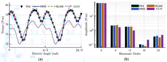
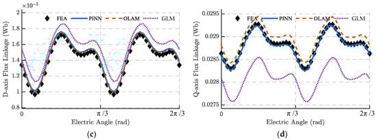
Figure 10.
Torque and armature flux linkage under the SE condition computed by the FEA, PINN, OLAM, and GLM methods: (a) torque waveform; (b) torque FFT; (c) d-axis flux linkage; (d) q-axis flux linkage (, ).
4.4.2. Torque Calculation Under USE Conditions
During the actual operation of the PMSM, due to a series of nonlinear factors such as inverter dead zone effect, the three-phase currents cannot be completely sinusoidal and contains harmonic components. To verify the validity of the PMSM nonlinear mathematical model and the PINN model in solving the torque under USE conditions, the harmonic currents are injected based on the second operating point. Table 4 shows the magnitude and phase of the injected harmonics of each order, and
Table 4.
Injected current harmonics.
Figure 11 shows the three-phase current excitation and waveforms of and after harmonic injection.
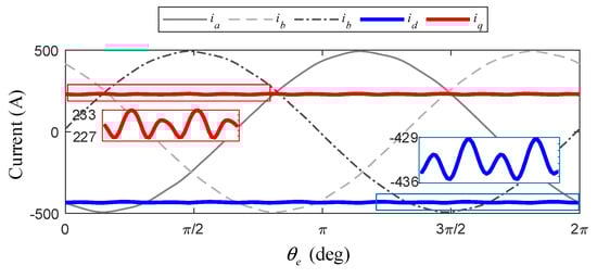
Figure 11.
Current waveform under USE condition.
Figure 12 presents a comparison of the torque and flux linkage results obtained by the GLM, PINN, and OLAM methods against those from FEA. Among the three, GLM exhibits the largest deviation, with an EDS reaching 27.02. The PINN model predicts torque more accurately than OLAM—its outputs align closely with non-FEA sampling points, as anticipated from the SE condition analysis. Specifically, OLAM yields a maximum torque error of 1.28 and an EDS of 6.8, whereas PINN reduces these to 0.37 and 1.52, corresponding to just 22% and 29% of the OLAM values, respectively. Apart from the 18th-order harmonic, PINN also outperforms OLAM in estimating both average torque and the amplitude of each harmonic order, as shown in Figure 12.
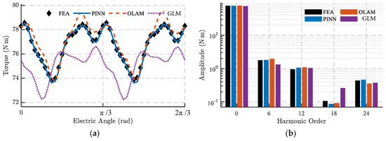
Figure 12.
Torque and armature flux linkage under the USE condition computed by the FEA, PINN, OLAM, and GLM methods: (a) torque waveform; (b) torque FFT.
5. Conclusions
This paper derives a nonlinear model of the PMSM based on differential inductance in both the ABC and dq0 frames. By treating current excitation and electrical angle as independent variables, the model establishes analytical expressions for inductance, magnetic flux linkage, magnetic energy, and torque, though iron losses and high-frequency eddy current effects remain unmodeled limitations.
To address the limitations of classical torque models and local linearization approaches, this paper develops a Fourier coefficient PINN for flux linkage based on FEA data and periodic boundary conditions of PMSM physical quantities. This network not only fits numerical relationships of given sample points but also ensures specific differential relationships and boundary conditions between inputs and outputs, enabling gradient descent-based active optimization. Benefiting from the independence of Fourier coefficients, the network allows parallel training/computation and facilitates angular frequency domain analysis of the PMSM.
To verify the accuracy of the differential inductance-based nonlinear model, this paper compares PINN and FEA torque prediction results under both SE and USE conditions with local linearization schemes. Results demonstrate that the proposed nonlinear torque model achieves precise torque and torque ripple calculation. With the same number of FEA sampling points, the PINN model shows higher accuracy in torque prediction for non-FEA sampled operating points and under USE conditions.
Author Contributions
Methodology, X.W.; modeling, S.W. All authors have read and agreed to the published version of the manuscript.
Funding
This work was supported by the National Key Research and Development Program of China (Grant No. 2024YFB2504900, Subproject No. 2024YFB2504903). The project “Intrinsic Wide-Temperature-Range High-Specific-Energy Power Battery Technology” is administered by the Ministry of Science and Technology of China.
Institutional Review Board Statement
Not applicable.
Informed Consent Statement
Not applicable.
Data Availability Statement
The raw data supporting the conclusions of this article will be made available by the authors on request.
Conflicts of Interest
The authors declare no conflicts of interest.
References
- Loganayaki, A.; Kumar, R.B. Permanent Magnet Synchronous Motor for Electric Vehicle Applications. In Proceedings of the 2019 5th International Conference on Advanced Computing & Communication Systems (ICACCS), Coimbatore, India, 15–16 March 2019; pp. 1064–1069. [Google Scholar] [CrossRef]
- Li, Y.; Gao, X.; Qin, Y.; Du, J.; Guo, D.; Feng, X.; Lu, L.; Han, X.; Ouyang, M. Drive Circuitry of an Electric Vehicle Enabling Rapid Heating of the Battery Pack at Low Temperatures. iScience 2021, 24, 101921. [Google Scholar] [CrossRef] [PubMed]
- Zhu, C.; Han, J.; Zhang, H.; Lu, F.; Liu, K.; Zhang, X. Modeling and Control of an Integrated Self-Heater for Automotive Batteries Based on Traction Motor Drive Reconfiguration. IEEE J. Emerg. Sel. Top. Power Electron. 2023, 11, 384–395. [Google Scholar] [CrossRef]
- Welchko, B.A.; Jahns, T.M.; Hiti, S. IPM Synchronous Machine Drive Response to a Single-Phase Open Circuit Fault. IEEE Trans. Power Electron. 2002, 17, 764–771. [Google Scholar] [CrossRef]
- Zhong, Z.; Jiang, S.; Zhou, Y.; Zheng, S. Magnetic Co-energy Based Modelling of PMSM for HEV/EV Application. Prog. Electromagn. Res. M 2016, 50, 11–22. [Google Scholar] [CrossRef]
- Feng, G.; Lai, C.; Kar, N.C. A Novel Current Injection-Based Online Parameter Estimation Method for PMSMs Considering Magnetic Saturation. IEEE Trans. Magn. 2016, 52, 8100404. [Google Scholar] [CrossRef]
- Liang, W.; Fei, W.; Luk, P.C.K. An Improved Sideband Current Harmonic Model of Interior PMSM Drive by Considering Magnetic Saturation and Cross-Coupling Effects. IEEE Trans. Ind. Electron. 2016, 63, 4097–4104. [Google Scholar] [CrossRef]
- Dietz, A.; Caruso, M.; Di Tommaso, A.O.; Miceli, R.; Nevoloso, C. Enhanced Mathematical Modelling of Interior Permanent Magnet Synchronous Machine Considering Saturation, Cross-Coupling and Spatial Harmonics Effects. In Proceedings of the 2020 Fifteenth International Conference on Ecological Vehicles and Renewable Energies (EVER), Monte-Carlo, Monaco, 10–12 September 2020; pp. 1–9. [Google Scholar]
- Li, H.; Zhang, J.; Luo, Y.; Wang, H.; Cui, X.; Dou, X. Finite Element Analysis of PMSM Steady State Parameters Considering Cross-Saturation Effect. Proc. CSEE 2012, 32, 104–110. [Google Scholar]
- Richter, J. Modellbildung, Parameteridentifikation und Regelung hoch Ausgenutzter Synchronmaschinen; Karlsruher Institut für Technologie (KIT): Karlsruhe, Germany, 2016. [Google Scholar]
- Meyer, M. Wirkungsgradoptimierte Regelung hoch Ausgenutzter Permanentmagnet-Synchronmaschinen im Antriebsstrang von Automobilen; Universität Stuttgart: Stuttgart, Germany, 2010. [Google Scholar]
- Shah, S.H.; Wang, Y.-C.; Shi, D.; Shen, J.-X. Investigation of Torque and Reduction of Torque Ripples through Assisted-Poles in Low-Speed, High-Torque Density Spoke-Type PMSMs. Machines 2024, 12, 327. [Google Scholar] [CrossRef]
- Weidenholzer, G.; Silber, S.; Jungmayr, G.; Bramerdorfer, G.; Grabner, H.; Amrhein, W. A Flux-Based PMSM Motor Model Using RBF Interpolation for Time-Stepping Simulations. In Proceedings of the 2013 International Electric Machines & Drives Conference, Chicago, IL, USA, 12–15 May 2013; pp. 1418–1423. [Google Scholar]
- Rahman, K.M.; Hiti, S. Identification of Machine Parameters of a Synchronous Motor. IEEE Trans. Ind. Appl. 2005, 41, 557–565. [Google Scholar] [CrossRef]
- Nakao, N.; Akatsu, K. Suppressing Pulsating Torques: Torque Ripple Control for Synchronous Motors. IEEE Ind. Appl. Mag. 2014, 20, 33–44. [Google Scholar] [CrossRef]
- Lee, G.-H.; Kim, S.-I.; Hong, J.-P.; Bahn, J.-H. Torque Ripple Reduction of Interior Permanent Magnet Synchronous Motor Using Harmonic Injected Current. IEEE Trans. Magn. 2008, 44, 1582–1585. [Google Scholar] [CrossRef]
- Rezaee-Alam, F. On-Load Cogging Torque Calculation in Surface-Mounted Permanent Magnet Motors Using Hybrid Analytical Model. IEEE Trans. Magn. 2024, 60, 8200110. [Google Scholar] [CrossRef]
- Wang, X.; Yi, P.; Zhou, Z.; Sun, Z.; Ruan, W. Improvements in the Permanent Magnet Synchronous Motor Torque Model Using Differential Inductance. IET Electr. Power Appl. 2020, 14, 109–118. [Google Scholar] [CrossRef]
- Karniadakis, G.E.; Kevrekidis, I.G.; Lu, L.; Perdikaris, P.; Wang, S.; Yang, L. Physics-Informed Machine Learning. Nat. Rev. Phys. 2021, 3, 422–440. [Google Scholar] [CrossRef]
- Hu, H.; Qi, L.; Chao, X. Physics-Informed Neural Networks (PINN) for Computational Solid Mechanics: Numerical Frameworks and Applications. Thin-Walled Struct. 2024, 205, 112495. [Google Scholar] [CrossRef]
- Li, X.; Deng, J.; Wu, J.; Zhang, S.; Li, W.; Wang, Y.-G. Physical Informed Neural Networks with Soft and Hard Boundary Constraints for Solving Advection-Diffusion Equations Using Fourier Expansions. Comput. Math. Appl. 2024, 159, 60–75. [Google Scholar] [CrossRef]
- Xia, C.; Du, B.; Huang, W.; Cui, S. Parameter Identification of Permanent Magnet Synchronous Motor Based on Physics-Informed Neural Network. In Proceedings of the 2024 5th International Conference on Power Engineering (ICPE), Shanghai, China, 13 December 2024; pp. 207–212. [Google Scholar]
- Zeng, Y.; Xiao, Z.; Liu, Q.; Liang, G.; Rodriguez, E.; Zou, G.; Zhang, X.; Pou, J. Physics-Informed Deep Transfer Reinforcement Learning Method for the Input-Series Output-Parallel Dual Active Bridge-Based Auxiliary Power Modules in Electrical Aircraft. IEEE Trans. Transp. Electrif. 2025, 11, 6629–6639. [Google Scholar] [CrossRef]
- Cuomo, S.; Di Cola, V.S.; Giampaolo, F.; Rozza, G.; Raissi, M.; Piccialli, F. Scientific Machine Learning Through Physics–Informed Neural Networks: Where We Are and What’s Next. J. Sci. Comput. 2022, 92, 88. [Google Scholar] [CrossRef]
- Wang, X.; Wang, H.; Liu, Y.; Li, Y.; Wang, P. Multi-Objective Control Harmonic Current Solution for Permanent Magnet Synchronous Motor. In Proceedings of the 2022 IEEE Transportation Electrification Conference and Expo, Asia-Pacific (ITEC Asia-Pacific), Haining, China, 28 October 2022; pp. 1–6. [Google Scholar]
- Hendriks, J.; Jidling, C.; Wills, A.; Schön, T. Linearly Constrained Neural Networks. arXiv 2021, arXiv:2002.01600. [Google Scholar]
- Lu, L.; Meng, X.; Mao, Z.; Karniadakis, G.E. DeepXDE: A Deep Learning Library for Solving Differential Equations. SIAM Rev. 2021, 63, 208–228. [Google Scholar] [CrossRef]
Disclaimer/Publisher’s Note: The statements, opinions and data contained in all publications are solely those of the individual author(s) and contributor(s) and not of MDPI and/or the editor(s). MDPI and/or the editor(s) disclaim responsibility for any injury to people or property resulting from any ideas, methods, instructions or products referred to in the content. |
© 2025 by the authors. Licensee MDPI, Basel, Switzerland. This article is an open access article distributed under the terms and conditions of the Creative Commons Attribution (CC BY) license (https://creativecommons.org/licenses/by/4.0/).