Differentiated GNSS Baseband Jamming Suppression Method Based on Classification Decision Information

Featured Application

The algorithm proposed in this paper has been used in the National Key Research and Development Plan project to achieve the application of GNSS receiver landing and third-party testing; the next planned step is to release an open source version to access the wide-area spatial and temporal network service platform in the form of SDK.

Abstract

In complex urban electromagnetic environments, wireless positioning signals are subject to various types of interference, including narrowband, chirp, and pulse jamming. Traditional generic suppression methods struggle to achieve global optimization tailored to specific interference mechanisms. This paper proposes a classification-driven differentiated jamming suppression (CDDJ) method, which adaptively selects the optimal mitigation strategy by pre-identifying interference types and integrating classification confidence levels. First, the theoretical bounds of the output carrier-to-noise ratio ($C/N_{0_{out}}$) under typical interference scenarios are derived, characterizing the performance distribution of anti-jamming efficiency ($\mathsf{\Gamma }$). Then, a mapping relationship between interference categories and their corresponding suppression strategies is established, along with decision criteria for strategy switching based on signal quality evaluation metrics. Finally, an OpenMax-Lite rejection layer is designed to handle low-confidence inputs, identify unknown jamming using the Weibull distribution, and implement a broadband conservative suppression policy. Simulation results demonstrate that the proposed method exhibits significant advantages across different interference types. Under high JSR conditions, the signal recovery rate improves by over 10% and 8% compared to that of the WPT and KLT methods, respectively. In terms of SINR performance, the proposed approach outperforms the AFF, TDPB, and FDPB methods by 1.5 dB, 1.1 dB, and 5.3 dB, respectively, thereby enhancing the reliability of wireless positioning in complex environments.

1. Introduction

In complex urban electromagnetic environments, the dense deployment of electronic devices poses multiple interference threats to wireless positioning signals [1]. Given the considerable distance between navigation satellites and the Earth, directly jamming the satellites themselves is extremely difficult. Consequently, ground-based navigation receivers become the most vulnerable component in the entire system link [2]. Since navigation signals utilize publicly known frequencies and structures and are subject to stringent power constraints, they undergo significant attenuation during atmospheric propagation. The long transmission distance further weakens the signal, resulting in extremely low power levels at the receiver, which makes it relatively easy to disrupt. Taking the BeiDou Navigation Satellite System (BDS) as an example, the signal power in the B1 band at the receiver is typically around −160 dBW. In more challenging environments, such as indoor spaces or urban canyons, the received signal strength may drop as low as −180 dBW [3]. Previous studies have shown that a suppression-type global navigation satellite system (GNSS) jammer with only 1 watt of power can cause significant interference to navigation signals within a radius of approximately 25 km [4]. Therefore, enhancing the interference resilience of satellite navigation receivers in complex electromagnetic environments is critical for improving their anti-jamming performance and ensuring the availability of navigation services.

The core of interference diagnosis lies in the real-time perception and accurate classification of interference events, serving as a decision-making foundation for anti-jamming strategies. Based on the observability of signal features, external interference can be categorized into map-observable and non-observable types. The former exhibits identifiable patterns in feature domains such as the time–frequency spectrum and the power spectrum, and typically includes suppression jamming (e.g., narrowband blocking), time–frequency domain spoofing (e.g., pseudocode delay/frequency shift modulation), and non-line-of-sight multipath interference. The latter encompasses highly covert mimicking spoofing and unmedicable signal disruptions, which lack distinguishable representations in conventional feature spaces.

GNSS malicious interference generally includes suppression-type and deception-type interference. Regarding suppression interference, traditional interference suppression techniques primarily include spatial domain filtering, temporal domain filtering, and transform domain filtering. In recent years, researchers have applied spatial adaptive processing (SAP) technology to the field of GNSS receiver anti-interference. The core idea of this technology is to optimize the antenna pattern by adaptively adjusting the weighting coefficients of the array antenna, thereby filtering out interference signals in the spatial domain while maintaining high gain for the target signal. Classic spatial adaptive filtering methods primarily include the maximum signal-to-interference ratio (MSIR), minimum mean square error (MMSE), and minimum variance (MV) methods [5]. Among these, the minimum variance method is further subdivided into two categories: minimum variance distortionless response (MVDR) and power inversion (PI). Additionally, by introducing time-domain delay lines to extend spatial processing, the space-time adaptive processing (STAP) method is constructed, which further increases system degrees of freedom and enhances interference resistance [6]. However, the STAP method typically requires a large array size, increasing the antenna size of the receiver as well as manufacturing and maintenance costs, making it unsuitable for portable or device-size-constrained applications.

Time-domain anti-jamming techniques suppress interference by exploiting the temporal characteristics distinguishing the positioning signal from jamming signals. These techniques are mainly categorized into two types. Pulse blanking performs well in sparse interference scenarios by setting an amplitude threshold to zero out signals exceeding the limit, offering low hardware implementation costs [7]. Adaptive filtering schemes, which include infinite impulse response (IIR) and finite impulse response (FIR) structures, leverage the recursive nature of IIR filters to achieve lower computational complexity and superior statistical properties. However, due to the temporal overlap between positioning and interference signals, this method may result in the loss of useful time-domain information from the navigation signal when facing certain types of interference [8].

Transform-domain methods project mixed signal data into the time–frequency or feature subspace by selecting reversible mappings that maximize signal-to-interference separability in the transform domain. These methods suppress various types of interference through techniques such as zeroing or subspace projection, without requiring additional hardware and while preserving the capability for signal reconstruction. Common transform techniques include short-time Fourier transform (STFT) [9,10], wavelet transform (WT) [11,12], and Karhunen–Loève transform (KLT) [13,14,15]. Although transform-domain approaches enhance interference energy compression and separation via frequency domain, time–frequency domain, or orthogonal basis decomposition, their deployment in dynamic and complex environments faces several common limitations:

(1)

Different interference types require specific configurations of window length, mother wavelet type, or energy thresholds for optimal suppression. When cross-domain changes occur—such as variations in interference power levels or channel fading—preset parameters struggle to adapt synchronously, leading to either insufficient suppression bandwidth (resulting in residual leakage) or excessive bandwidth that inadvertently degrades the desired signal [16,17].

(2)

Transform-domain separation typically assumes significant energy differences between the signal and interference along at least one feature dimension. When the legitimate signal and interference exhibit similar energy levels in localized time–frequency regions, overly high thresholds may cause signal loss, while low thresholds allow interference sidelobes to persist, making it difficult to maintain consistent separation using fixed thresholds or projection dimensions.

(3)

Conventional transform-domain methods primarily target energy-based interference and lack capabilities for spoofing feature recognition or alerting. Spoofed components may remain latent in the observed data after transform processing, rendering subsequent filters unaware of degraded signal integrity, thereby continuously injecting false position information into the navigation solution and accumulating systemic bias [18,19].

To address these challenges, this paper proposes a classification-driven differentiated jamming suppression (CDDJ) method, which incorporates prior knowledge of known interference types and associated confidence scores into the suppression process [20]. First, the theoretical upper and lower bounds of the output carrier-to-noise ratio ($C/N_{0_{out}}$) under representative interference scenarios are derived, revealing variations in the distribution of anti-jamming efficiency (Γ) and establishing the performance limits of unified suppression algorithms. Next, a mapping relationship is constructed between known interference types and their corresponding dedicated suppression algorithms, and an anti-jamming decision-switching criterion is formulated based on signal quality evaluation metrics. Finally, for inputs with insufficient confidence, a lightweight OpenMax-Lite rejection layer is appended to the end of the diagnostic network. This layer estimates the probability of unknown interference via the tail distribution of the Weibull function, based on class center distances. If this estimated probability exceeds a predefined threshold, or if the SoftMax confidence score falls below a set limit, the input is classified as unknown interference, and a broadband conservative suppression strategy is triggered.

The remainder of this paper is organized as follows. Section 2 introduces typical interference signal models. Section 3 provides a detailed description of the proposed interference suppression method, covering both known and unknown interference types. Section 4 presents simulation experiments to evaluate the suppression performance of the CDDJ method under various interference conditions, including chirp, pulse, and narrowband jamming, along with an in-depth experimental analysis. Finally, Section 5 concludes the paper.

2. Jamming Classification and Mathematical Modeling

Due to significant attenuation over long-distance transmission, GNSS signals arrive at the receiver with extremely low power. Although direct sequence spread spectrum (DSSS) techniques enhance signal concealment, the overall anti-jamming margin remains limited. In complex electromagnetic environments, GNSS receivers are highly susceptible to external interference, which may result in signal acquisition failure, loss of lock, or positioning drift. External interference can be categorized into two types based on its origin:

• Environmental interference, which arises from non-line-of-sight (NLOS) propagation and signal blockage or interruption caused by dense urban structures or complex terrain.
• Man-made interference, which includes:

Jamming, where energy-based disruptions degrade receiver performance. Typical forms include amplitude modulation (AM) jamming, frequency modulation (FM) jamming, chirp (swept-frequency) jamming, narrowband (NB) blocking, and pulsed interference, as shown in Figure 1.

Spoofing, where counterfeit signals with code phase, carrier frequency, and Doppler parameters similar to the authentic signals are transmitted to mislead the receiver into producing erroneous navigation solutions.

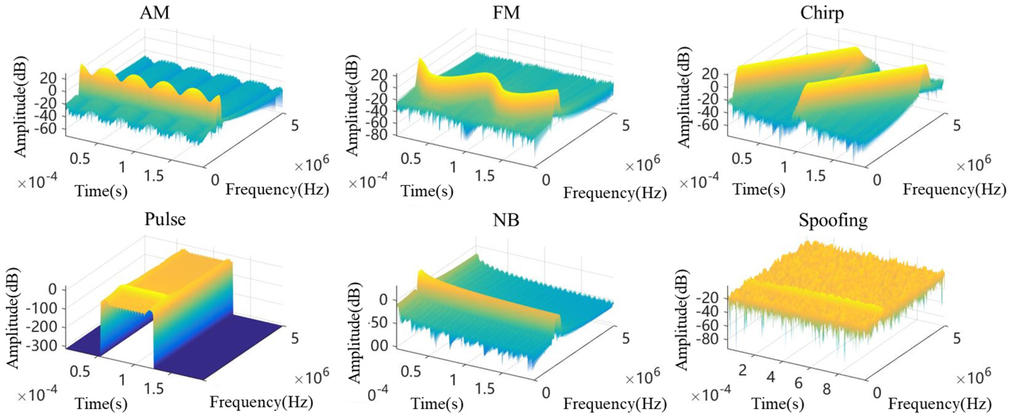
2.1. Suppressive Jamming

(1)

Amplitude modulation (AM) jamming: As a subclass of continuous wave (CW) interference, AM jamming can be categorized into single-tone and multi-tone modulation types. Its defining characteristic lies in the carrier amplitude being modulated by a low-frequency signal. The interference at the $n$-th sampling point can be expressed as [20]

$$z_{am}[n]=Pp[n]\otimes \sum _{k=1}^{M_a}{R}_{p_k}\mathrm{e}\mathrm{x}\mathrm{p}\left(j\left(2\pi f_{p_k}nT+{\theta }_{p_k}\right)\right)$$

(1)

In this expression, $M_a$ denotes the number of amplitude-modulated tones. $P$ is the interference gain factor derived from the jamming signal ratio (JSR), representing the power ratio between the interference and the GNSS signal.$p\left[n\right]$ denotes the channel coefficient vector of the suppressive interference link, and $\otimes$ represents the convolution operator, accounting for multipath fading effects within the interference channel. $R_{p_k}$, $f_{p_k}$, and ${\theta }_{p_k}$ represent the amplitude, frequency, and phase of the $k$-th AM interference component, respectively.

(2)

Frequency modulation (FM) jamming: This type of interference features a time-varying carrier frequency, characterized by a large instantaneous bandwidth and low power spectral density. Such properties enable it to effectively evade adaptive filtering and frequency-domain notch filtering strategies at the receiver. It is defined as [20]

$$z_{fm}[n]=Pp[n]\otimes \sum _{k=1}^{M_f}a\cdot \mathrm{e}\mathrm{x}\mathrm{p}\left(j\left(2\pi f_{m_k}nT+{\beta }_k\mathrm{s}\mathrm{i}\mathrm{n}\left(2\pi f_{m_k}nT\right)\right)\right)$$

(2)

$M_f$ denotes the number of multi-tone carriers, $f_{m_k}$ is the frequency of the $k$-th jamming component, and ${\beta }_k$ is the modulation index of the $k$-th carrier.

(3)

Chirp jamming: Its instantaneous frequency periodically sweeps over a predefined frequency band within a short time interval and resets at the end of each cycle. Common forms include linear chirp jamming and sinusoidally modulated chirp jamming, defined as follows [20]:

$$z_{cp}[n]=Pp[n]\otimes \mathrm{e}\mathrm{x}\mathrm{p}\left(j\left(2\pi f_{ch}nT+\pi a{\displaystyle \frac{f_{max}-f_{min}}{T_{swp}}}{\theta }_c\right)\right)$$

(3)

$f_{ch}$ is the initial sweep frequency, $f_{min}$ and $f_{max}$ define the lower and upper bounds of the sweep bandwidth, respectively, $T_{swp}$ is the time taken to sweep from $f_{min}$ to $f_{max}$, $a\in \{+1,-1\}$ is a random variable used to determine the sweep direction, and ${\theta }_c$ is the initial phase of the chirp jamming signal.

(4)

Narrowband jamming: This refers to the injection of narrowband interference components with power significantly higher than the useful GNSS signal within the main frequency band. Its bandwidth is typically narrower than the main lobe bandwidth of the GNSS signal. The spectral expression is given by [20]

$$\mathsf{\Omega }(f)=\left\{\begin{array}{cc}\mu ,\left|f-f_0\right|<B/2& \\ 0,\mathrm{o}\mathrm{t}\mathrm{h}\mathrm{e}\mathrm{r}\mathrm{w}\mathrm{i}\mathrm{s}\mathrm{e}& \end{array}\right.$$

(4)

Here, $\mu$, $f_0$, and $B$ represent the amplitude, center frequency, and bandwidth of the narrowband jamming signal, respectively. By passing a stationary random process through a band-pass filter, the time-domain expression of the interference, $\omega \left[n\right]$, is obtained. Its convolution with the pseudocode sequence of the navigation signal, $p\left[n\right]$, is given by $z_{nb}\left[n\right]=Pp\left[n\right]\otimes \omega \left[n\right]$.

(5)

Pulse jamming: This type of interference periodically generates multiple pulses within a fixed repetition interval, each with a certain duty cycle. It is characterized by short duration, significant spectral spreading, and high peak power. It is typically modeled as a series of Gaussian-shaped pulse pairs, expressed as [20]

$$z_{pl}[n]=Pp[n]\otimes \sum _{k=1}^{M_p}{\alpha }_{k}u\left(nT-{\eta }_k\right)\mathrm{e}\mathrm{x}\mathrm{p}\left(j2\pi f_k\left(nT-{\eta }_k\right)\right)$$

(5)

In this expression, $u(\cdot )$ represents the waveform of a single pulse, $M_p$ is the number of pulses per unit time, and ${\alpha }_k$, $f_k$, and ${\eta }_k$ denote the amplitude, carrier frequency, and time delay parameter of the $k$-th pulse, respectively.

2.2. Spoofing

Based on the number of transmitters, spoofing can be categorized into single-source and multi-source types; according to the signal generation method, it can be divided into replay-based and generative spoofing, and it can be classified into simple, moderate, and advanced levels of interference complexity.

(1)

Simple spoofing adopts a two-step strategy of “jamming first, then spoofing”. When a navigation terminal is already locked onto authentic satellite signals, it will maintain tracking as long as the code delay and Doppler shift of the spoofed signal fall outside the pull-in range of the tracking loop. Therefore, the attacker must first transmit high-power jamming signals to cause the receiver to lose lock. After maintaining the jamming for a certain period, the transmitter switches to broadcasting the spoofed signal. Once the terminal loses lock, it attempts reacquisition based on historical parameters and due to the power advantage of the spoofed signal, it locks onto it and includes it in the PVT solution. Thus, in single-interference-source scenarios, it can be assumed that suppression and spoofing interference, as well as different categories of suppression jamming signals, do not occur simultaneously.

(2)

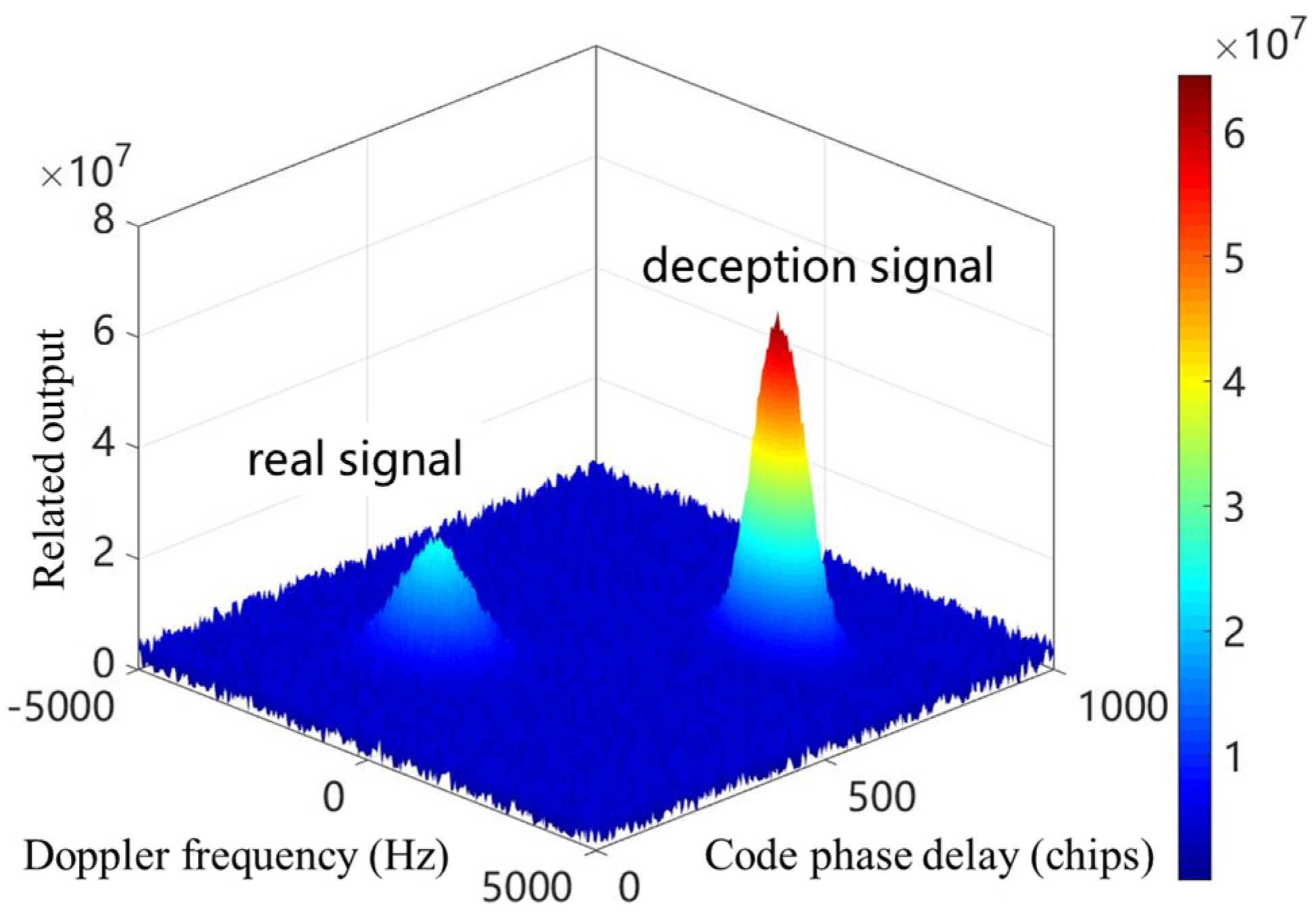
Moderate-level spoofing achieves takeover without loss of lock by aligning the spoofed signal’s code phase and Doppler frequency with those of the authentic signal. The spoofing device first receives genuine satellite signals and estimates the relative position and velocity of the target receiver. It then generates spoofed signals with identical parameters and transmits them in an overlapping manner. As the spoofed signal gradually increases in power and introduces a slow code phase shift, the receiver’s tracking loop becomes dominated by the stronger spoofed signal, ultimately leading to takeover of the positioning solution. During this process, the receiver remains locked, making detection difficult and the spoofing highly covert.

(3)

Advanced-level spoofing extends moderate spoofing by introducing multiple transmitters. Each antenna independently simulates the signal of a specific satellite, collectively forming a spatial signal field that closely mimics real satellite geometry, thereby enhancing the resistance to multi-antenna spoofing detection techniques. However, due to the complexity of transmission synchronization, phase control, and environmental dynamics, practical implementation remains highly challenging, and engineering feasibility is currently low. As a result, this form of spoofing does not yet pose a significant real-world threat.

Considering the combined effects of channel fading, Doppler shift, and phase offset, this section extends the diagnostic targets to include high-power delay/frequency-shift spoofing with observable features, as well as complex scenarios involving changes in the number of GNSS signals. Spoofed and authentic GNSS signals typically use the same PRN pseudorandom code sequence but embed falsified navigation message bits, expressed as

$$z_{sp}[n]=\sum _{k=1}^K{G}_k{q}_k[n]\otimes {\widehat{d}}_k\left(nT-{\delta }_k\right)c_k\left(nT-{\delta }_k\right)\mathrm{c}\mathrm{o}\mathrm{s}\left(2\pi f_{kp}nT+{\psi }_k\right)$$

(6)

In this expression, $G_k$ is the gain factor determined by the spoofing signal-to-noise power ratio, $q_k\left[n\right]$ is the channel coefficient vector of the spoofing link corresponding to the $k$-th PRN code, and ${\widehat{d}}_k$ denotes the falsified navigation message information being transmitted. ${\delta }_k$, $f_{kp}$, and ${\psi }_k$ represent the time delay, Doppler frequency offset, and phase deviation of the $k$-th spoofed signal, respectively.

In the absence of interference, the received signal consists only of authentic navigation signals and additive white Gaussian noise. Since the power of the GNSS signals is significantly lower than the noise floor during the correlation preprocessing stage, the power spectral density of the composite signal is dominated by characteristics of white Gaussian noise.

3. Proposed Jamming Suppression Method

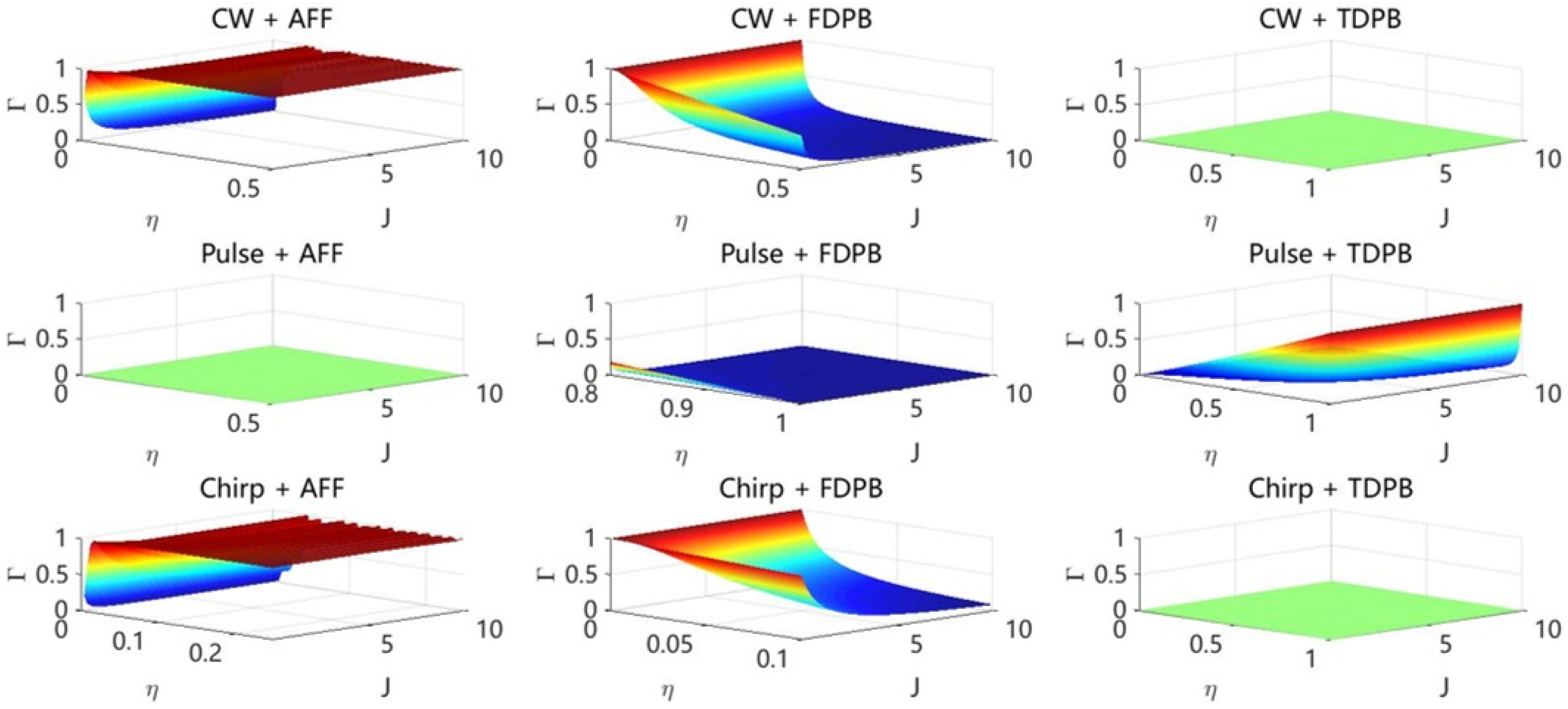
3.1. Analysis of Performance Degradation Under a Unified Suppression Strategy

Different interference scenarios exhibit markedly distinct statistical characteristics, making it difficult for a single suppression strategy—lacking a tailored design for specific interference mechanisms—to achieve global optimality. Even for the same type of interference, different algorithms can yield significantly different suppression results. Without incorporating specialized reception structures, such as antenna arrays or polarization-based systems, conventional positioning receivers typically rely on three representative interference suppression techniques: frequency domain pulse blanking (FDPB), time domain pulse blanking (TDPB), and adaptive FIR filtering (AFF).

(1)

FDPB

The received signal is mapped from the time domain to the frequency domain using the discrete Fourier transform (DFT) method:

$$X(k)=\sum _{n=0}^{N-1}x(n)e^{-\mathrm{j}2\pi {\displaystyle \frac{kn}{N}}}$$

(7)

Here, $N$ denotes the transform length. If the interference exhibits sparsity in the frequency domain, appearing as localized spectral anomalies, effective suppression can be achieved by eliminating spectral distortion through nonlinear filtering. However, threshold selection is constrained by the non-stationary nature of receiver noise. Following the approach in [21], let $Y\left(k\right)=X\left(k\right)/\left|X\right(k\left)\right|$ to remove the dependence on prior information. The processed spectrum is then transformed back to the time domain using the inverse discrete Fourier transform (IDFT) mtehod, yielding the interference-suppressed signal.

$$y(n)={\displaystyle \frac{1}{N}}\sum _{k=0}^{N-1}Y(k)e^{j2\pi {\displaystyle \frac{kn}{N}}}$$

(8)

(2)

TDPB

TDPB operates directly on the sampled signal using a threshold-free strategy, with the processing procedure given by [21]:

$$y(n)={\displaystyle \frac{x\left(n\right)}{\left|x\right(n\left)\right|}}$$

(9)

(3)

AFF

AFF adaptively adjusts the filter coefficients to automatically generate notches in the interference bands for suppression. Let L be the order of the FIR filter; its output is expressed as [22]

$$y(n)=\sum _{k=0}^{L-1}x(n-k)h^{\left(n\right)}(L-k)$$

(10)

Here, $h^{\left(n\right)}\left(k\right)$ denotes the $k$-th coefficient of the FIR filter at time $n$. The filter coefficients are iteratively updated using the normalized least mean squares (NLMS) algorithm [22]:

$$h^{(n+1)}(k)=h^{\left(n\right)}(k)-{\displaystyle \frac{\mu }{|x(n){|}^2}}x(n)(y(n){)}^{*}$$

(11)

$\mu$ is the normalized step-size factor, and $(\cdot {)}^{*}$ denotes the complex conjugate operation. The coefficient update is driven by $y\left(n\right)$; a larger $\mu$ results in faster convergence but higher steady-state error, while a smaller $\mu$ leads to slower convergence with improved steady-state accuracy. In the simulation experiments, $\mu$ = 0.1 is selected as an empirical value.

To comprehensively evaluate the performance of various suppression methods under different interference conditions, three typical jamming scenarios are constructed and subjected to 1000 Monte Carlo simulations: narrowband jamming (bandwidth: 0–4 MHz, occupying 20% of the BDS receiver signal bandwidth); pulse jamming (repetition period: 0.04–1 ms, duty cycle: 0–40%, modulated by band-limited noise); chirp jamming (sweep bandwidth: 4–20 MHz, sweep period: 0.01–1 ms). For each type of interference, suppression is performed using the FDPB, AFF, and TDPB strategies, respectively. The output signal’s $C/N_0$ is statistically analyzed to assess the suppression performance of each algorithm.

Figure 2 compares the algorithm performance across the three interference scenarios. Under narrowband jamming, AFF and FDPB exhibit similar $C/N_0$ improvement, while TDPB yields the lowest $C/N_0$ due to insufficient frequency-domain resolution. In the case of pulse jamming, TDPB performs the best, owing to its advantage in time-domain pulse shaping, achieving a mean $C/N_0$ of 37.7 dB/Hz; FDPB follows, while AFF performs the worst due to its lack of transient response capability. For chirp jamming, TDPB shows the poorest performance (mean $C/N_0$ of 23.8 dB/Hz); FDPB outperforms AFF when $C/N_0$ is below 41 dB/Hz, whereas AFF surpasses FDPB beyond this threshold. The simulation results indicate that the optimal algorithm choice is highly scenario-dependent, and even within the same interference type, different parameter configurations may lead to varying optimal suppression strategies.

The interference suppression performance is evaluated using the output carrier-to-noise ratio, defined as $C/N_{0_{out}}=S/(N+J_{res})$, where $J_{res}$ denotes the residual interference power. The ideal upper bound is achieved when $J_{res}=0$, resulting in $\mathrm{C}/{\mathrm{N}}_{0_{max}}=S/N$. However, most methods incur unavoidable residual loss. The lower bound is given by ${\left(C/N_0\right)}_{min}=S/(N+\eta J)$, where $\eta$is the leakage factor. The theoretical upper and lower bounds of $C/N_{0_{out}}$ for each algorithm under typical interference conditions are derived, as shown in

Table 1. Theoretical upper and lower bounds of $C/N_{0_{out}}$ for FDPB, TDPB, and AFF under typical disturbances.

Jamming	Algorithm	${\left(\mathit{C}/{\mathit{N}}_0\right)}_{\mathit{m}\mathit{a}\mathit{x}}$	${\left(\mathit{C}/{\mathit{N}}_0\right)}_{\mathit{m}\mathit{i}\mathit{n}}$
NB	AFF	$S/N$	$S/(N+{\left({\displaystyle \frac{\pi L}{2}}{\displaystyle \frac{\delta f}{f_s}}\right)}^2{J}_{res})$
	FDPB	$S/(N+{\displaystyle \frac{n_{min}\Delta f_{bin}}{B_{int}}}{J}_{res})$	$S/(N+{\displaystyle \frac{n\Delta f_{bin}}{B_{int}}}{J}_{res})$
	TDPB	$S/(N+J_{res})$
Pulse	AFF	$S/(N+J)$
	FDPB	$S/(N+{\eta }_{min}{J}_{res})$	$S/(N+\eta J)$
	TDPB	$S/\left(N\right(1-D\left)\right)$	$S/(N+\left(1-D_{eff}\right)J_{res})$
Chirp	AFF	$S/(N+J)$	$S/(N+(1-{\displaystyle \frac{\Delta f_{notch}}{B_{chirp}}})J_{res})$
	FDPB	$S/(N+{\displaystyle \frac{n_{min}\Delta f_{bin}}{B_{chirp}}}{J}_{res})$	$S/(N+{\displaystyle \frac{n\Delta f_{bin}}{B_{chirp}}}{J}_{res})$
	TDPB	$S/(N+J)$

. In the table, $\delta f$ represents the frequency offset between the notch and the interference center, $\Delta f_{bin}=f_s/N_{FFT}$ is the frequency resolution, $B_{int}$ and $B_{chirp}$ denote the interference and chirp bandwidths, respectively, $n$ is the number of missed bins under the threshold, $n_{min}$ is the theoretical minimum number of missed bins, $D$ is the pulse duty cycle, and $\Delta f_{notch}$ is the effective bandwidth of the notch filter. The normalized anti-jamming efficiency coefficient is defined as follows.

$$\mathsf{\Gamma }={\displaystyle \frac{{\left(C/N_0\right)}_{alg}-{\left(C/N_0\right)}_{min}}{{\left(C/N_0\right)}_{max}-{\left(C/N_0\right)}_{min}}},\mathsf{\Gamma }\in [0,1]$$

(12)

Here, ${\left(C/N_0\right)}_{alg}$ represents the actual output carrier-to-noise ratio. Figure 3 quantifies the anti-jamming efficiency $\mathsf{\Gamma }$ under varying leakage factors $\eta$ and interference power levels $J$. Γ is defined as a normalized performance metric representing the effectiveness of interference suppression, relative to the theoretical optimum ($\mathsf{\Gamma }=1$) and the unsuppressed case ($\mathsf{\Gamma }=0$). The value of Γ reflects the degree of structural alignment between the algorithm and the interference characteristics, as well as the suppression capability. When $\mathsf{\Gamma }$ approaches 1, the algorithm performance nears the ideal limit; when $\mathsf{\Gamma }$ approaches 0, it indicates suppression failure. For example, TDPB achieves the highest $\mathsf{\Gamma }$ value under pulse jamming, whereas its mean $\mathsf{\Gamma }$ under the chirp and narrowband interference scenarios is close to 0, confirming the varying sensitivity of its time-domain processing mechanism to different interference dynamics.

During satellite signal acquisition, the maximum correlation peak occurs when the parameters of the real signal match those of the local replica signal. Deception signals also exhibit peak characteristics when they meet the same parameter matching conditions. When the power of the deception signals is significantly higher than that of real signals, their correlation peaks will dominate, leading to the risk of false locking by the receiver. Under conditions where the deception interference and BDS signals coexist at the same frequency, the statistical characteristics of the mixed signal detection can be represented as a superposition model of the real signal component and the interference component.

$$V_t=G\cdot \mathrm{s}\mathrm{i}\mathrm{n}\mathrm{c}\left(\pi \Delta f{T}_d\right)\cdot \sqrt{{\displaystyle \frac{P}{2}}\left[R_c^2\left({\tau }_k-\widehat{\tau }\right)+k^2{R}_c^2\left({\delta }_k-\widehat{\tau }\right)\right]+2k\cdot R_c\left({\tau }_k-\widehat{\tau }\right)R_c\left({\delta }_k-\widehat{\tau }\right)\mathrm{c}\mathrm{o}\mathrm{s}\left(\Delta {\varphi }_m\right)}$$

(13)

where $G={f_{s}T}_d$ is the gain factor, $P$ is the true signal power, $\Delta f$ is the estimated frequency difference, $\widehat{\tau }$ is the estimated delay, $\Delta {\varphi }_m$ is the phase difference between the spoofing and true signals, $R_c(\cdot )$ denotes the correlation function, and $k$ is the interference relative power factor. Figure 4 simulates the two-dimensional search results of a GNSS receiver under spoofing interference. Under conditions where the spoofing signal power dominates, the amplitude of its main correlation peak significantly exceeds the true signal peak, causing the receiver to produce a false lock phenomenon.

When the receiver captures a spoofing interference signal with a power higher than that of the true signal, it will incorrectly adopt the initial code phase and Doppler shift of the spoofing signal into the tracking loop, causing the spoofing signal to interfere with the DLL and PLL. Under conditions where spoofing interference and true signals coexist, the outputs of the in-phase and quadrature branches of the GNSS receiver’s tracking loop correlator can be represented as three coherent integral values, E, P, and L, where the P branch is

$$\begin{gathered} I_P\approx {\displaystyle \frac{\sqrt{2P}}{2}}R\left({\tau }_c-{\tau }_k\right)\mathit{cos}\left({\varphi }_k-{\varphi }_c\right)+{\displaystyle \frac{\sqrt{2P}}{2}}kR\left({\tau }_c-{\delta }_k\right)\mathit{cos}\left({\psi }_k-{\varphi }_c\right) \\ {Q}_P\approx {\displaystyle \frac{\sqrt{2P}}{2}}R\left({\tau }_c-{\tau }_k\right)\mathrm{s}\mathrm{i}\mathrm{n}\left({\varphi }_k-{\varphi }_c\right)+{\displaystyle \frac{\sqrt{2P}}{2}}kR\left({\tau }_c-{\delta }_k\right)\mathrm{s}\mathrm{i}\mathrm{n}\left({\psi }_k-{\varphi }_c\right) \end{gathered}$$

(14)

where ${\tau }_c$ and ${\varphi }_c$ represent the delay and phase of the local code, respectively. A non-normalized power difference DLL phase detector is used, with the following discrimination function:

$$D_D(\epsilon )={\displaystyle \frac{1}{2}}\left[\left(I_E^2+Q_E^2\right)-\left(I_L^2+Q_L^2\right)\right]={\displaystyle \frac{P}{4}}\left[R^2\left(\epsilon +{\displaystyle \frac{D}{2}}\right)-R^2\left(\epsilon -{\displaystyle \frac{D}{2}}\right)\right]$$

(15)

where $D$ is the distance between correlators. In steady-state operation, $D_D\left(\epsilon \right)=0$ is satisfied. In the case of spoofing interference, there exists

$$\begin{array}{cc}\hfill D_D^{’}(\epsilon )=& D_D(\epsilon )+{\displaystyle \frac{P}{4}}{k}^2\left[R^2\left(\epsilon +{\displaystyle \frac{D}{2}}-{\tau }_m\right)-R^2\left(\epsilon -{\displaystyle \frac{D}{2}}-{\tau }_m\right)\right]\hfill \\ & +{\displaystyle \frac{P}{2}}k\cos \left({\varphi }_m\right)\left[R\left(\epsilon +{\displaystyle \frac{D}{2}}\right)R\left(\epsilon +{\displaystyle \frac{D}{2}}-{\tau }_m\right)-R\left(\epsilon -{\displaystyle \frac{D}{2}}\right)R\left(\epsilon -{\displaystyle \frac{D}{2}}-{\tau }_m\right)\right]\hfill \end{array}$$

(16)

In the equation, ${\tau }_m$ and ${\varphi }_m$ represent the time delay difference and phase difference between the spoofing signal and the real signal, respectively. The above equation shows that the DLL tracking error mainly depends on the power of the spoofing interference signal, the phase difference between the spoofing signal and the real signal, the autocorrelation characteristics of the spread spectrum code, and the relative code phase deviation between the two signals.

The mechanism by which spoofing interference affects the tracking loop is similar to that of multipath effects. When the relative delay is less than approximately 1.5 chips, the interference signal distorts the discrimination function, causing additional tracking errors. However, when the delay exceeds this threshold, the receiver misinterprets the spoofing interference as a real signal and achieves stable locking.

Under the assumption that the linear pseudo range observation model holds, the effects of pseudo range disturbances introduced by each satellite on the receiver’s position solution can be considered as linear superpositions. A two-satellite spoofing interference scenario was constructed using the Badious system’s PRN2 and PRN5 satellites, with the maximum spoofing slope in the negative X direction of the receiver (geometric sensitivity coefficients: PRN2 = −0.8, PRN5 = −0.6). In the simulation, the pseudo range extension values of the two satellites were linearly scanned within the range of 0 to 100 m to analyze the impact of different pseudo range extension combinations on positioning errors. The results in Figure 2, Figure 3, Figure 4, Figure 5 and Figure 6 show that the error in the X direction exhibits an enhanced trend, with a slope of −1.4. When the pseudo range extensions of both satellites are 100 m, and the positioning error along the X axis reaches 140 m, accounting for 94.7% of the total positioning error. This validates the decisive influence of multi-satellite spoofing interference on the receiver’s position error, with the extent of error amplification constrained by the spatial geometric relationship between the satellites and the receiver.

3.2. Directed Suppression Strategies with Known Interference Types

This section innovatively establishes the mapping relationship between the interference and suppression algorithms and proposes a decision switching criterion based on signal quality evaluation. We design a targeted suppression strategy based on the classification label and the confidence score ${\tau }_{con}$ output by the interference diagnosis module. When the interference is of a known type and ${\tau }_{con}\ge {\tau }_t$, the system activates a parameterized suppressor matched to the interference category; otherwise, it switches to an open-set conservative suppression mode.

According to the degree of alignment between the interference types and suppression methods, a mapping relationship is constructed, as shown in

Table 2. Mapping between interference types and suppression algorithms.

Jamming	Preferred	Alternative	Estimated Parameters	Estimation Method
AM	AFF	FDPB	$f_p,M_a$	FFT + Hilbert
FM	FDPB	FDPB	$f_{\mathrm{c}}\left(t\right),{\dot{f}}_{\mathrm{c}}$	FFT + PLL
Chirp	FDPB	AFF	$f_{start},f_{stop},{\dot{f}}_c$	STFT + Hough
NB	AFF	FDPB	$f_0$	FFT single-peak
Pulse	TDPB	FDPB	$t_k,{\eta }_k$	Time-domain CFAR

. Since spoofing interference involves the imitation and confusion of false satellite signals, once spoofing is confirmed, the system excludes the contaminated satellite signals from the positioning solution and activates the integrity protection algorithm to recalculate the protection level, thereby ensuring the trustworthiness of the navigation output.

Considering that parameter estimation errors and the dynamic range of excessive interference may lead to failure of the initial suppression strategy, this paper constructs a two-level anti-jamming decision framework by adding a signal quality feedback control layer above the diagnostic layer (see Figure 6). Within each monitoring window ${\mathcal{W}}_k=\left\{t_k-m{T}_s,\dots ,t_k\right\}$, sliding estimates of the frequency-domain $\widehat{C/N_0}(k)$, DLL discriminator variance ${\sigma }_{\mathrm{D}\mathrm{L}\mathrm{L}}^2\left(k\right)$, and residual interference power ratio $\widehat{\eta }\left(k\right)$ are performed, and a loss function is constructed.

$$L\left(k\right)=\sum _{i=1}^3{w}_i\left(k\right)\cdot {\displaystyle \frac{{\nu }_i\left(k\right)-{\nu }_{i,n\mathrm{o}\mathrm{m}}}{{\nu }_{i,th}-{\nu }_{i,\mathrm{n}\mathrm{o}\mathrm{m}}}},\sum _{i=1}^3{w}_i(k)=1$$

(17)

${\nu }_{n\mathrm{o}\mathrm{m}}$ denotes the nominal value, and ${\nu }_{th}$ is the lower bound under failure conditions. Based on historical data $\left\{x_{ij}\right\}$, the probability distribution is calculated as $p_{ij}=x_{ij}/\sum _{i=1}^n{x}_{ij}$, which is then used to compute the initial weight allocation:

$$w_j\left(0\right)={\displaystyle \frac{1-E_j}{\sum _{l=1}^3\left(1-E_l\right)}}, E_j=-{\displaystyle \frac{1}{\ln n}}\sum _{i=1}^n{p}_{ij}\mathrm{l}\mathrm{n}{p}_{ij}$$

(18)

The weights are updated every $T_{ad}=20$ s using a sliding mean.

$${\overline{\nu }}_j={\displaystyle \frac{1}{m_{ad}}}\sum _{i=k-m_{ad}+1}^k{\nu }_j(i)$$

(19)

Here, $m_{ad}=T_{ad}/T_s$, and the weight update is given by

$$w_j(k)={\displaystyle \frac{w_j(k-1)\left[1+\alpha \left({\nu }_j\left(k\right)-{\overline{\nu }}_j\right)\right]}{\sum _{l=1}^3{w}_l(k-1)\left[1+\alpha \left({\nu }_l\left(k\right)-{\overline{\nu }}_l\right)\right]}}$$

(20)

The adjustment factor $\alpha$ is set within the range [0.05, 0.1]. Three suppression states are defined: Primary, Backup, and Conservative broadband. After obtaining the composite loss $L\left(k\right)$ within the monitoring window, it is compared against fixed thresholds.

(1)

Upgrade condition: if $L\left(k\right)\ge 1$, the suppression state escalates to the next level (Primary → Backup, or Backup → Conservative).

(2)

Downgrade condition: if already in a higher-level state and $L\left(k\right)\le 0.9$, the Backup state immediately downgrades to Primary, while the Conservative state downgrades after persisting for 60 ms.

(3)

All other cases: the current suppression state is maintained.

3.3. A Framework for Unknown Interference Open Set Detection and Conservative Suppression

Since the domain alignment module significantly tightens the feature distribution of known classes, the SoftMax layer may produce high-confidence misclassifications for unknown interference. To address this, a lightweight OpenMax-Lite rejection module is appended to the output of the interference diagnosis network. This module relies solely on the distance between a sample and the predicted class center and estimates the probability of unknown interference using the Weibull distribution fitted to the tail of known class features. If the estimated unknown probability exceeds a predefined threshold or the predicted confidence falls below the set limit, the input is classified as unknown interference, and the system switches to conservative broadband suppression.

Assume the interference set is defined as $\mathcal{C}=\{\mathrm{AM}, \mathrm{FM}, \mathrm{Chirp}, \mathrm{C}\mathrm{W},\mathrm{Pulse}, \mathrm{spoofing}\}$. The logits output vector from the back end of the diagnostic network is denoted as $\mathbf{z}(x)\in {\mathbb{R}}^M$, and the domain-aligned intermediate feature is $\mathbf{f}(x)\in {\mathbb{R}}^D$. The decision is made as follows:

$$J(x)=\left\{\begin{array}{c}1,x\in C\\ 0,x\notin C\end{array}\right.$$

(21)

If$J=0$, the system switches to the conservative broadband suppression path.

(1)

Offline phase: class center and tail distribution modeling.

Feature center:

$${\mathbf{c}}_j={\displaystyle \frac{1}{N_j}}\sum _{x\in {\mathcal{C}}_j}\mathbf{f}\left(x\right),j\in \mathcal{C}$$

(22)

Here, $N_j$ is the number of samples for class $j$ in the training set, and the distance is measured as $d_j\left(x\right)={‖\mathbf{f}\left(x\right)-{\mathbf{c}}_j‖}_2$. For each class, the top 20% of the largest values from the distance sequence $\left\{d_j\right\}$ are selected to form the set ${\mathcal{T}}_j$. The cumulative distribution function (CDF) of the Weibull distribution is

$$F_j(d)=1-\mathrm{e}\mathrm{x}\mathrm{p}\left[-{\left({\displaystyle \frac{d}{{\lambda }_j}}\right)}^{k_j}\right],d\ge 0$$

(23)

Here, $\left({\lambda }_j,k_j\right)$ are the scale and shape parameters of the Weibull distribution, obtained via maximum likelihood estimation.

(2)

Online detection phase:

For the SoftMax output vector $\mathbf{p}\left(x\right)=\left[p_1,p_2,\dots ,p_M\right]$, the predicted label is $\widehat{y}=\mathrm{a}\mathrm{r}\mathrm{g}\underset{j}{\mathrm{m}\mathrm{a}\mathrm{x}}{p}_j(x)$, with confidence threshold ${\tau }_t$. Based on the Weibull distribution parameters $\left({\lambda }_{\widehat{y}},k_{\widehat{y}}\right)$ fitted from the tail samples of class $\widehat{y}$, the probability that the sample falls outside the trusted region is calculated as $P_{\mathrm{u}\mathrm{n}\mathrm{k}}\left(x\right)=F_{\widehat{y}}\left(d_{\widehat{y}}\left(x\right)\right)$. If ${\tau }_{con}<{\tau }_t$ or $P_{unk}\left(x\right)\ge {\tau }_f$, the input is classified as unknown interference. To determine ${\tau }_t$ and ${\tau }_f$, a separate validation dataset is used to compute the true positive rate (TPR) and false positive rate (FPR) under different thresholds, generating the ROC curve. The optimal threshold is selected based on the maximum Youden index:

$$\mathrm{a}\mathrm{r}\mathrm{g}\underset{\mathrm{x}}{\mathrm{m}\mathrm{a}\mathrm{x}}[\mathrm{T}\mathrm{P}\mathrm{R}(x)-\mathrm{F}\mathrm{P}\mathrm{R}(x)]$$

(24)

KLT suppression does not rely on the interference type or spectral priors. Instead, it estimates the overall covariance of the received signal and performs eigen-decomposition to extract the dominant energy directions that form the interference subspace. Although its suppression performance is inferior to that of targeted suppressors when the interference type is known, it can still significantly reduce leakage of the dominant power components and suppress broadband interference backgrounds in unknown interference scenarios. The procedure is as follows:

(1)

For the sample data block ${\mathbf{y}}_n\in {\mathbb{C}}^{L\times 1}$ within the $n$-th window, the covariance matrix is updated as

$${\widehat{\mathbf{R}}}_n=\alpha {\widehat{\mathbf{R}}}_{n-1}+(1-\alpha ){\mathbf{y}}_n{\mathbf{y}}_n^{\mathrm{H}},0<\alpha <1$$

(25)

(2)

Decompose the updated covariance matrix ${\widehat{\mathbf{R}}}_n$ as

$${\widehat{\mathbf{R}}}_n={\mathbf{U}}_n{\mathsf{\Lambda }}_n{\mathbf{U}}_n^{\mathrm{H}},{\mathsf{\Lambda }}_n=\mathrm{d}\mathrm{i}\mathrm{a}\mathrm{g}\left({\lambda }_1\ge \dots \ge {\lambda }_L\right)$$

(26)

(3)

The interference subspace dimension is estimated using the minimum description length (MDL) criterion:

$$\widehat{q}=\&\underset{q}{\mathrm{a}\mathrm{r}\mathrm{g}\mathrm{m}\mathrm{i}\mathrm{n}}\left[-\log \left(\prod _{i=q+1}^L{\lambda }_i\right)+\left(L-q\right)\cdot \right.\left.\log \left({\displaystyle \frac{1}{L-q}}\sum _{i=q+1}^L{\lambda }_i\right)+{\displaystyle \frac{1}{2}}q\left(2L-q\right)\mathrm{l}\mathrm{o}\mathrm{g}{N}_R\right]$$

(27)

where $N_R=1/(1-\alpha )$.

(4)

Let the eigenvectors corresponding to the interference subspace be ${\mathbf{U}}_q=\left[{\mathbf{u}}_1,\dots ,{\mathbf{u}}_q\right]$, and its orthogonal complement be ${\mathbf{U}}_q^{\perp }=\left[{\mathbf{u}}_{q+1},\dots ,{\mathbf{u}}_L\right]$. The projection matrix is constructed as

$${\mathbf{P}}_{\mathit{K}\mathit{L}\mathit{T}}={\mathbf{U}}_q^{\perp }{\left({\mathbf{U}}_q^{\perp }\right)}^{\mathrm{H}}$$

(28)

The filtered output is then given by

$${\tilde{\mathbf{y}}}_n={\mathbf{P}}_{\mathit{K}\mathit{L}\mathit{T}}{\mathbf{y}}_n$$

(29)

The KLT suppression method primarily targets low-rank, high-power interference, but it may still exhibit blind spots when dealing with sparsely distributed multi-tone peak interference in the frequency spectrum. To address this limitation, a wideband adaptive frequency filter (AFF-WB) module is further introduced. This module performs compensation-based suppression of spectral peak interference without relying on prior parameters, using autonomous spectral peak detection and fixed-template notch filter construction. The processing flow is as follows:

(1)

Let $S_n\left[k\right]={\mathrm{F}\mathrm{F}\mathrm{T}}_K\left\{{\tilde{\mathbf{y}}}_n\right\}$ and the average power spectrum be ${\overline{P}}_n$. A frequency bin k is selected if it satisfies

$$10{\mathrm{l}\mathrm{o}\mathrm{g}}_{10}\left({\left|S_n\left[k\right]\right|}^2/{\overline{P}}_n\right)\ge {\gamma }_{\mathrm{p}\mathrm{k}}$$

(30)

Record the spectral peak as $f_m=k{F}_s/N$, where ${\gamma }_{\mathrm{p}\mathrm{k}}$ is the threshold for peak detection in the spectrum.

(2)

For each peak frequency, construct a pair of fixed-bandwidth poles as $a_m=r{e}^{j2\pi f_m/F_s}$. All notch filters are cascaded to form the overall transfer function

$$H(z)=\prod _{m=1}^M{\displaystyle \frac{1-a_m{z}^{-1}}{1-\frac{a_m}{\left|a_m\right|}{z}^{-1}}}$$

(31)

(3)

The time-domain filtered output is given by

$${\mathbf{y}}_n^{\mathrm{A}\mathrm{F}\mathrm{F}}=H\left(z\right){\tilde{\mathbf{y}}}_n$$

(32)

To address potential processing overhead issues, the proposed framework was designed with computational efficiency and hardware deployment feasibility in mind. The classification module employs a lightweight OpenMax-Lite rejection mechanism, achieving inference times within 20 milliseconds on an ARM Cortex-A72 CPU. The decision switching logic is based on low-complexity signal quality statistics and is updated every 100 milliseconds, which is fully within the standard GNSS positioning cycle update interval. For the suppression module, all algorithms (such as AFF, FDPB, and TDPB) are implemented using minimized window sizes and optimized matrix operations.

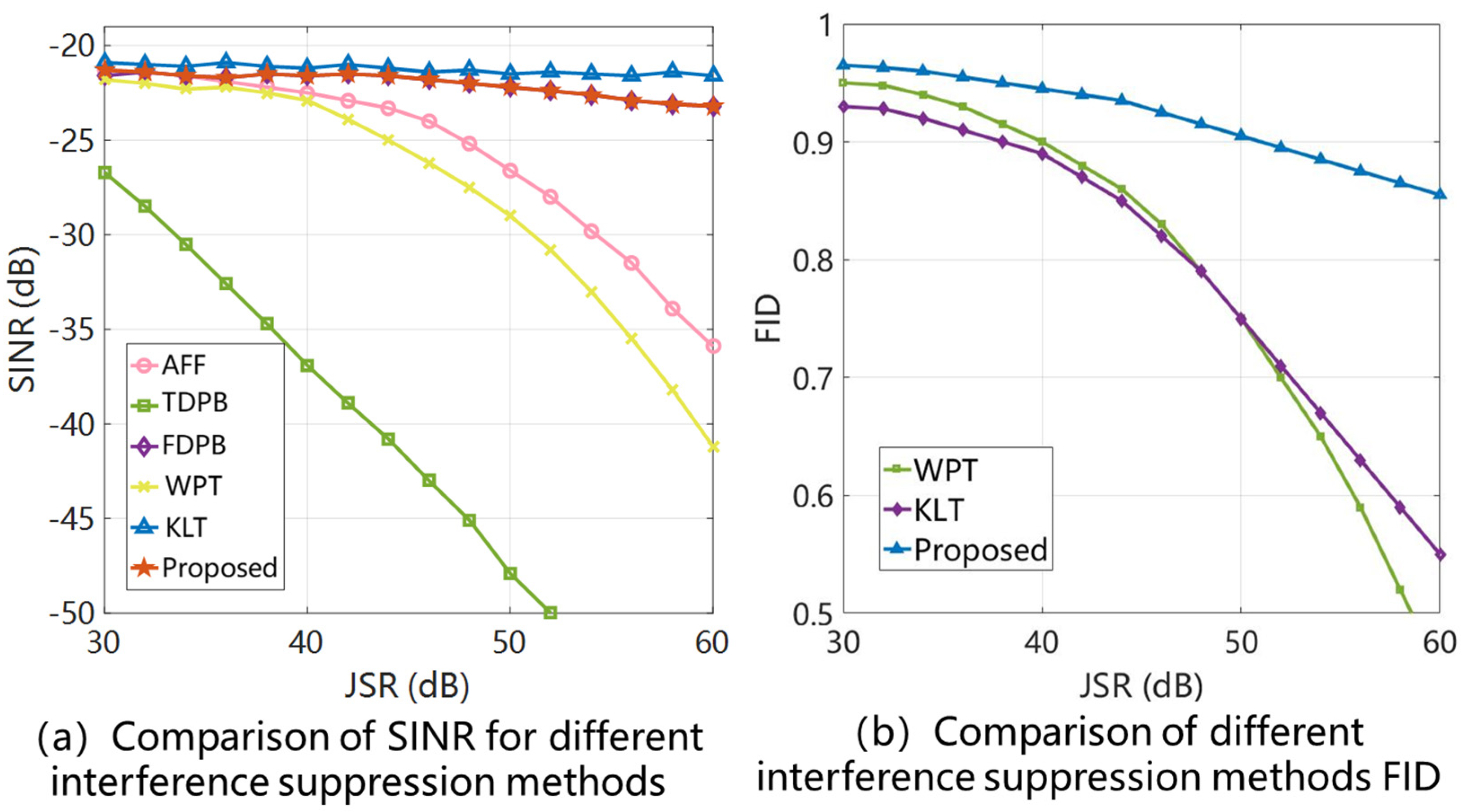
4. Results

This section validates the proposed algorithm through simulation experiments. The experiment simulates a typical Badious B1 signal (1561.1 MHz) with a sampling rate of 20 MHz. The RF front-end performs down-conversion on the received satellite RF signal to generate an intermediate frequency (IF) analog signal, which is then digitized by an A/D converter to produce a digital IF sequence. The noise-free signal at the $n$-th sampling instant is modeled as

$$S_I[n]=\sum _{k=1}^K{A}_k{d}_k\left(nT-{\tau }_k\right)c_k\left(nT-{\tau }_k\right)\mathrm{c}\mathrm{o}\mathrm{s}\left(2\pi \left(f_I+f_{d_k}\right)nT+{\varphi }_k\right)$$

(33)

In this expression, $T=1/f_s$ is the sampling period, $f_s$ is the sampling frequency, and $f_I$ is the intermediate frequency. $K$ denotes the number of visible satellites, and $A_k$ and ${\tau }_k$ represent the amplitude and time delay of the $k$-th satellite signal, respectively. $c_k(\cdot )$ and $d_k(\cdot )$ are the pseudorandom spreading sequence and the navigation data modulation waveform, respectively. $f_{d_k}$ and ${\varphi }_k$ denote the Doppler shift and phase offset of the $k$-th signal, respectively. After downsampling, the signal is transformed to baseband. Assuming $f_I=0$, the sampled signal at time index $n$ is re-expressed as

$$y[n]={\sum }_{k=1}^K{A}_k{h}_k[n]d_k\left(nT-{\tau }_k\right)c_k\left(nT-{\tau }_k\right)\mathrm{c}\mathrm{o}\mathrm{s}\left(2\pi f_{d_k}nT+{\varphi }_k\right)+z[n]+v[n]$$

(34)

Here, $h_k\left[n\right]$ denotes the time-varying channel response of the $k$-th propagation path, $z\left[n\right]$ is the interference component, and $v\left[n\right]$ is independent and identically distributed Gaussian noise with zero mean and variance ${\sigma }^2=N_0{f}_s/2$, where $N_0$ is the one-sided power spectral density of the noise.

Each signal may include 1 to 5 multipath components with decreasing power, and their delays are uniformly distributed within one pseudocode period. It is assumed that there is a single interference source in the environment. All interference signals are randomly generated within predefined parameter spaces and superimposed with the GNSS signal to form composite samples.

Table 3. Definition of interference parameter space.

Jamming	Parameter Setting
AM	$f_{p_k}~\mathcal{U}(1558,1564)$ MHz, $m~\mathcal{U}(0.2,0.8)$
FM	$f_{m_k}~\mathcal{U}(0.5,2.0)$ MHz, ${\beta }_k~\mathcal{U}(0.2,1.0)$
Chirp	$f_{start}~\mathcal{U}(1558,1564)$ MHz, $\mathsf{\Delta }f\sim \mathcal{U}\left(1,25\right)$ MHz, $T_{\mathrm{s}\mathrm{w}\mathrm{p}}~\mathcal{U}(0.05,5)$ ms,$a=\pm 1$
NB	$f_0~\mathcal{U}(1558,1564)$ MHz, $B~\mathcal{U}(50,300)$ kHz
Pulse	${\alpha }_k\sim \mathcal{U}\left(0.8,1.2\right),a_k\sim \mathcal{U}\left(0.02,1\right) \mathsf{\mu }\mathrm{s},$ $T_p\sim \mathcal{U}\left(2,10\right)\mathsf{\mu }\mathrm{s},M_p=⌊1\mathrm{m}\mathrm{s}/T⌋$,$D=1/T_p{\sum }_{k=1}^{M_p}{a}_k$

defines the parameter space for each type of interference, where $\mathcal{U}(\mathrm{a},\mathrm{b})$ denotes a uniform distribution over the interval $[\mathrm{a},\mathrm{b}]$.

By comparing the performance of AFF, TDPB, FDPB, WPT-based interference suppression, KLT-based interference suppression, and the proposed method under various types of interference, the effectiveness of the proposed approach is validated. To evaluate the interference mitigation performance of the proposed model, three key metrics are considered:

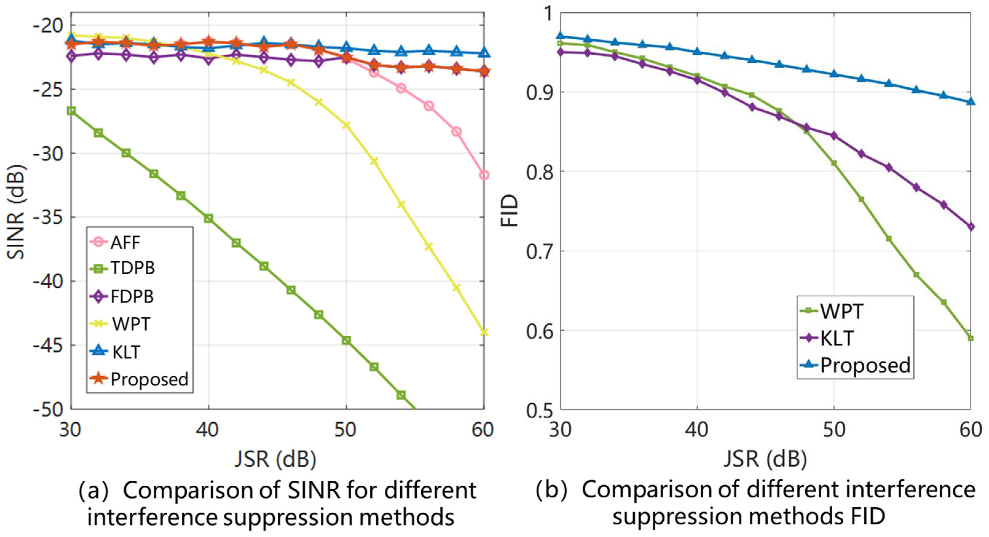
(1)

SINR: used to assess the steady-state performance after interference suppression;

(2)

FID: measures the degree to which the model preserves GNSS signal integrity.

$${\mathrm{F}\mathrm{I}\mathrm{D}}_{\mathrm{d}\mathrm{B}}=10{\mathrm{l}\mathrm{o}\mathrm{g}}_{10}\left({\displaystyle \frac{\sum _n{y}^2\left(n\right)}{\sum _n\left(\widehat{y}\right(n)-y(n){)}^2}}\right)$$

(35)

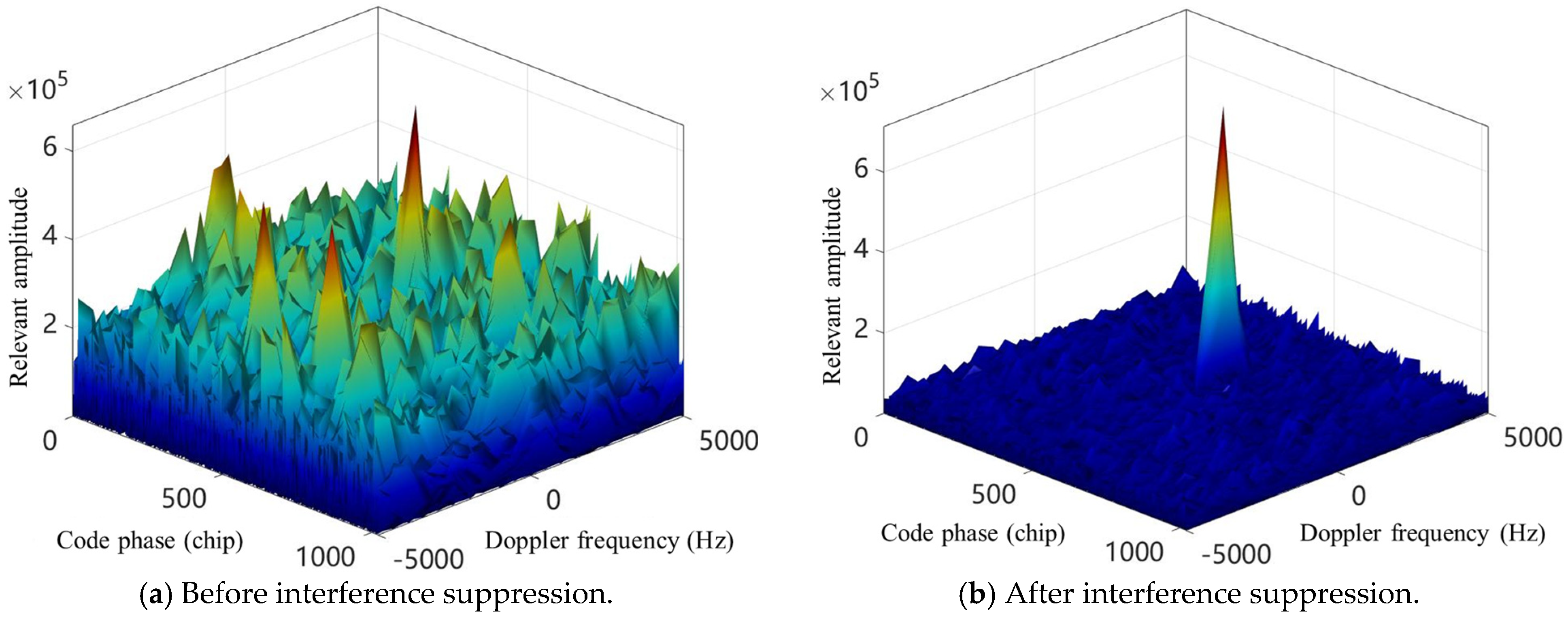
(3)

CAF: employs the cross-ambiguity function to evaluate signal acquisition capability.

The nominal $C/N_0$ of BDS B1 code is 43 dB/Hz (corresponding to an SNR of approximately −20 dB). Although its direct sequence spread spectrum (DSSS) scheme provides nearly 30 dB of spreading gain, signal acquisition remains highly susceptible to suppression interference. When the in-band interference power exceeds the dynamic range of the receiver, an increase in JSR leads to a sharp decline in the equivalent carrier-to-noise ratio ${\left[C/N_0\right]}_{eq}$, which manifests as follows:

$${\left[C/N_0\right]}_{eq}=-10\mathrm{l}\mathrm{o}\mathrm{g}\left[{10}^{-\left(C/N_0\right)/10}+{\displaystyle \frac{{10}^{(J/S)/10}}{Q{R}_c}}\right]$$

(36)

A spreading factor of Q = 1 indicates narrowband interference, while Q = 2 represents wideband interference. The signal acquisition threshold is set at 28 dB/Hz. Figure 7 illustrates the evolution curve of ${\left[C/N_0\right]}_{eq}$ with increasing JSR. The simulation results show that when the interference power exceeds the signal power by approximately 34.9 dB, the receiver reaches a critical state of acquisition failure.

This section evaluates the interference suppression performance of the proposed method through 100 independent Monte Carlo simulation runs. Figure 8a presents the SINR performance under a narrowband single-tone interference scenario, comparing the proposed method with several existing suppression algorithms, including AFF, FDPB, TDPB, KLT, and WPT, across varying interference intensities (JSR levels). The simulation results show that while all methods exhibit a certain degree of suppression capability against single-tone interference, the output SINR of each algorithm generally degrades as the interference power (JSR) increases. This trend is primarily due to the increasing difficulty of suppression under stronger interference conditions. In contrast, the proposed method incorporates a diagnostic analysis module that dynamically selects the most suitable suppression sub-algorithm based on the diagnosed interference type, thereby achieving more stable and superior performance across the entire JSR range. Compared to AFF, FDPB, and TDPB, the proposed method achieves average SINR improvements of 0.9 dB, 0.4 dB, and 16.9 dB, respectively. Notably, the substantial advantage over TDPB is attributed to its inherent weakness in dealing with narrowband interference, resulting in severely limited suppression effectiveness.

It is worth noting that although the KLT method demonstrates slightly better SINR performance than the proposed method under high JSR conditions, it suffers from a noticeable decline in FID. Figure 8b further analyzes the variation in FID across different algorithms, revealing that KLT exhibits a rapid decrease in FID as JSR increases. This phenomenon stems from the fact that KLT employs a fixed threshold to determine the retention of eigen components. When interference power is high, it becomes difficult to distinguish between interference-dominated and signal-dominated components, leading to the erroneous removal of eigenvectors containing useful signal energy, thereby compromising signal integrity. In contrast, WPT achieves relatively high FID under low JSR conditions due to its multi-band decomposition strategy. However, as interference strength increases, the spread of interference energy renders WPT’s fixed-band partitioning increasingly ineffective. Signal-containing bands are misclassified as interference, causing significant nonlinear distortion to the signal and a rapid drop in FID. Compared with these methods, the proposed approach adaptively identifies interference frequency regions and applies targeted frequency-domain projection suppression. This strategy effectively avoids misclassification and the unintended removal of signal bands, maintaining higher signal fidelity even under high JSR conditions. The simulation results show that at a JSR of 50 dB, the proposed method achieves FID improvements of 13.8% and 9.1% over WPT and KLT, respectively.

Figure 9 presents the performance comparison of different interference suppression methods under the chirp jamming scenario. The simulation results show that the proposed method consistently maintains excellent suppression performance, with only a slight degradation as JSR increases. Compared with the TDPF algorithm, the proposed method achieves an average SINR improvement of approximately 8 dB, highlighting the performance limitations of TDPF when dealing with frequency-varying chirp interference. Additionally, the KLT algorithm outperforms the proposed method by about 0.5 dB in regards to average SINR. However, it is noteworthy that KLT suffers a significant fidelity drop of approximately 17.1% at a JSR of 50 dB. This indicates that, despite KLT’s strong suppression capability, its fixed threshold mechanism may result in the unintended deletion of useful signal components. Overall, compared with other algorithms, the proposed method achieves a better balance between interference suppression and signal fidelity under chirp interference, effectively maintaining signal integrity while ensuring robust suppression performance.

Under 10 µs pulse interference conditions, 100 Monte Carlo simulations were conducted with a duty cycle of 20%, varying JSR between 30 and 60 dB, and the average SINR after suppression by each algorithm was calculated. The results in Figure 10 show that the average SINR of the method proposed in this paper is 3.0 dB higher than that of WPT, 19.8 dB higher than that of AFF, and 5.3 dB higher than that of FDPB. Figure 11 presents the performance comparison of the proposed algorithm under pulse jamming with different duty cycles (20%, 50%, and 80%). The simulation results indicate that increasing the duty cycle intensifies the impact of pulse jamming on the positioning signals. However, the proposed algorithm consistently demonstrates stable and effective suppression performance across all duty cycle conditions. Further analysis reveals that the influence of the duty cycle on algorithm performance is closely related to the JSR level. Under low JSR conditions, variations in duty cycle exert a more pronounced effect on the suppression performance of the TDPB algorithm, resulting in noticeable differences in SINR. As JSR increases and the interference energy becomes dominant, the performance gap caused by duty cycle variations gradually narrows.

Under chirp interference, the signal capture performance is typically evaluated based on the peak clarity in the cross ambiguity function (CAF). The clearer the peak in the CAF, the stronger the capture algorithm’s ability to locate the true Doppler frequency and pseudocode phase. Figure 11 compares the changes in the CAF before and after interference suppression processing, with the simulation conditions set as shown in

Table 4. Parameter settings for acquisition and tracking stage simulation.

No.	Parameter	Value	No.	Parameter	Value
1	Signal Type	GPS L1 C/A	7	Frequency Search Step Size	300 Hz
2	SNR	−20 dB	8	Tracking Duration	1 s
3	JNR	30 dB	9	DLL Loop Bandwidth	1 Hz
4	Doppler Frequency	1500 Hz	10	PLL Loop Bandwidth	10 Hz
5	Code Phase Offset	479 chips	11	FLL Loop Bandwidth	20 Hz
6	Code Phase Search Step Size	0.5 chip	12	Relevant Interval	1 s

.

As shown in Figure 12a, before interference suppression processing, the high-power interference components remaining in the received signal severely disrupted the peak structure in the CAF, making it difficult to distinguish the peaks corresponding to the true signal. This situation is likely to cause misjudgments by the capture module, resulting in incorrect Doppler frequency and pseudocode phase estimates. As shown in Figure 12b, interference suppression processing significantly improves the main-to-secondary peak ratio of the target signal, effectively suppressing interference residues in the background region. The main peak in the CAF becomes clearer and more distinguishable, thereby enhancing the accuracy of identifying the true pseudocode phase and Doppler frequency during the capture process and improving the accuracy and robustness of signal capture.

To further validate the performance of the interference suppression method proposed in this paper, a simulation analysis was conducted on the signal tracking performance after interference suppression. During the signal tracking phase, the coarse estimates of the signal Doppler frequency and pseudocode phase provided by the capture module were used as the initial input for the tracking loop. Through iterative correction by the loop filter, more precise measurement information was obtained, and the navigation message was demodulated. The frequency lock indicator (FLI) can be used to measure the frequency tracking performance of the frequency-locked loop (FLL) for the signal frequency, defined as

$$\mathrm{F}\mathrm{L}\mathrm{I}={\displaystyle \frac{{\mathrm{d}\mathrm{o}\mathrm{t}}^2-{\mathrm{c}\mathrm{r}\mathrm{o}\mathrm{s}\mathrm{s}}^2}{{\mathrm{d}\mathrm{o}\mathrm{t}}^2+{\mathrm{c}\mathrm{r}\mathrm{o}\mathrm{s}\mathrm{s}}^2}}$$

(37)

where

$$\begin{array}{c}\mathrm{dot}=I_{P,k-1}{I}_{P,k}+Q_{P,k-1}{Q}_{P,k}\\ \mathrm{cross}=I_{P,k-1}{Q}_{P,k}-Q_{P,k-1}{I}_{P,k}\end{array}$$

(38)

$I_{P,k}$ and $Q_{P,k}$ represent the prompt-related values of the in-phase and the quadrature branches in the kth integration cycle, respectively. The value range of FLI is [−1, 1]. When FLI approaches 1, it indicates that the frequency tracking is more stable and the accuracy is higher. The phase lock indicator (PLI) is used to evaluate the tracking accuracy of the PLL for the received signal carrier phase and is defined as

$$\mathrm{P}\mathrm{L}\mathrm{I}={\displaystyle \frac{I_{P,k}^2-Q_{P,k}^2}{I_{P,k}^2+Q_{P,k}^2}}$$

(39)

The PLI value ranges from −1 to 1. The closer it is to 1, the higher the PLL tracking accuracy. Figure 13 shows the time-dependent changes in FLI and PLI within the 0.1 s to 0.2 s interval. As shown in the figure, when using the time-domain blanking method to suppress chirp interference, the values of FLI and PLI randomly fluctuate within the range of [−1, 1], indicating that both FLL and PLL fail to achieve effective frequency and phase tracking, and the loop is in an unlocked state. In contrast, after applying the KLT method and the method proposed in this paper, the values of FLI and PLI both stabilize near 1, indicating that the FLL and PLL have reached steady-state operating conditions, enabling accurate tracking of the carrier frequency and phase, and demonstrating excellent interference suppression and robust signal tracking performance.

5. Discussion

In our previous work, the research team pioneered a cross-domain interference diagnosis approach based on knowledge transfer, which, to the best of our knowledge, marked the first application of domain generalization in the field of interference diagnosis. The related outcomes have been widely implemented in localized service platforms and 5G positioning terminals.

Building upon that foundation, the present study further investigates the mechanisms of interference suppression, analyzes the limitations of unified suppression strategies, and proposes a classification-driven differentiated interference suppression method. To validate its effectiveness, we compare the proposed approach with five representative baseline methods: AFF, TDPB, FDPB, KLT, and WPT. These baselines cover a broad range of commonly used GNSS anti-jamming strategies, including time-domain, frequency-domain, transform-domain, and subspace-based techniques. Experimental results demonstrate that our approach achieves low-complexity, real-time, and cost-effective interference mitigation, with significant performance improvements over that of classical methods such as KLT and WPT.

Looking forward, our goal is to further advance this suppression method toward hardware-level implementation and conduct real-world testing in complex urban environments. In addition, we note that the proposed method operates at the baseband signal processing level and maintains standard-compliant output formats (e.g., C/N₀, PVT), ensuring compatibility with existing GNSS receiver standards such as RTCA DO-229. It also preserves signal integrity under unknown interference, which supports downstream applications like precise timing and robust navigation.

6. Conclusions

This paper proposes a classification-driven differentiated jamming suppression method to address the diverse interference challenges encountered in high-precision GNSS positioning. By dynamically selecting the optimal suppression strategy—either through parameterized suppressors or an open-set conservative mode—based on the matching between interference type and suppression approach, the proposed method effectively overcomes the performance limitations of traditional generic suppression techniques in multi-interference scenarios. The experimental results demonstrate that the proposed approach achieves significant performance gains under various interference types, including narrowband, chirp, and pulse jamming. Moreover, it successfully balances suppression effectiveness and signal fidelity in high-JSR environments, achieving a comprehensive optimization of both interference mitigation and signal quality. Future research may further focus on improving the precision of spoofing interference detection and enhancing the adaptability of suppression modules in order to strengthen the system’s robustness in increasingly complex environments.

References

- Ren, B.; Chen, F.; Ni, S.; Han, C.; Lu, Z.; Han, S. Performance analysis of repeater spoofing suppression based on GNSS multi-beam receiver. Front. Phys. 2022, 10, 970132. [Google Scholar] [CrossRef]
- Yang, L.; Zhu, J.; Fu, Y.; Yu, Y. Integrity Monitoring for GNSS Precision Positioning. In Positioning and Navigation Using Machine Learning Methods; Springer: Berlin/Heidelberg, Germany, 2024; pp. 59–75. [Google Scholar]
- Chen, F. GNSS Antenna Array Receiver Interference Suppression and Measurement Deviation Compensation Technology; National University of Defense Technology: Changsha, China, 2017. [Google Scholar]
- Huang, S.; Guo, K.; Wang, Z.; Zhu, Y.; Tang, H.; Wang, Y. A dme interference signal identification and mitigation approach based on gaussian mixture model used for bds b2a receivers. In Proceedings of the 2023 IEEE/AIAA 42nd Digital Avionics Systems Conference (DASC), Barcelona, Spain, 1–5 October 2023; IEEE: Piscataway, NJ, USA, 2023; pp. 1–6. [Google Scholar]
- Ni, S.; Binbin, R.; Chen, F.; Lu, Z.; Wang, J.; Ma, P.; Sun, Y. GNSS spoofing suppression based on multi-satellite and multi-channel array processing. Front. Phys. 2022, 10, 905918. [Google Scholar] [CrossRef]
- Gioia, C. GNSS Navigation in Difficult Environments: Hybridization and Reliability. Ph.D. Thesis, University Parthenope of Naples, Naples, Italy, 2014. [Google Scholar]
- Ma, X.; Han, C.; Jin, R.; Wang, D.; Bai, P.; Zhen, W. Study on gnss spoofing interference detection method in urban multipath environment based on cnn and clustering model. In Proceedings of the 2023 Cross Strait Radio Science and Wireless Technology Conference (CSRSWTC), Guilin, China, 10–13 November 2023; IEEE: Piscataway, NJ, USA, 2023; pp. 1–3. [Google Scholar]
- Gioia, C.; Borio, D. A statistical characterization of the Galileo-to-GPS inter-system bias. J. Geod. 2016, 90, 1279–1291. [Google Scholar] [CrossRef]
- Borio, D.; Camoriano, L.; Lo Presti, L. Two-pole and multipole notch filters: A computationally effective solution for GNSS interference detection and mitigation. IEEE Syst. J. 2008, 2, 38–47. [Google Scholar] [CrossRef]
- Lineswala, P.L.; Shah, S.N. Performance analysis of different interference detection techniques for navigation with Indian constellation. IET Radar Sonar Navig. 2019, 13, 1207–1213. [Google Scholar] [CrossRef]
- Borio, D.; Gioia, C. Robust interference mitigation: A measurement and position domain assessment. In Proceedings of the 2020 International Technical Meeting of the Institute of Navigation, San Diego, CA, USA, 21–24 January 2020; pp. 274–288. [Google Scholar]
- Musumeci, L.; Dovis, F. Use of the wavelet transform for interference detection and mitigation in global navigation satellite systems. Int. J. Navig. Obs. 2014, 2014, 262186. [Google Scholar] [CrossRef]
- Park, K.; Lee, D.; Seo, J. Dual-polarized GPS antenna array algorithm to adaptively mitigate a large number of interference signals. Aerosp. Sci. Technol. 2018, 78, 387–396. [Google Scholar] [CrossRef]
- Kornblith, S.; Shlens, J.; Le, Q.V. Do better imagenet models transfer better? In Proceedings of the IEEE Computer Society Conference on Computer Vision and Pattern Recognition, Long Beach, CA, USA, 15–20 June 2019; pp. 2656–2666. [Google Scholar]
- Borio, D. Robust signal processing for GNSS. In Proceedings of the 2017 European Navigation Conference (ENC), Lousanne, Switzerland, 9–12 May 2017; pp. 150–158. [Google Scholar]
- Honig, M.L.; Poor, H.V. Adaptive interference suppression. In Wireless Communications: Signal Processing Perspectives; Prentice-Hall: Upper Saddle River, NJ, USA, 1998; pp. 64–128. [Google Scholar]
- Zhang, L.; Zhao, H.; Sun, C.; Bai, L.; Feng, W. Enhanced GNSS spoofing detector via multiple-epoch inertial navigation sensor prediction in a tightly-coupled system. IEEE Sens. J. 2022, 22, 8633–8647. [Google Scholar] [CrossRef]
- Hu, Y.; Bian, S.; Li, B.; Zhou, L. A novel array-based spoofing and jamming suppression method for GNSS receiver. IEEE Sens. J. 2018, 18, 2952–2958. [Google Scholar] [CrossRef]
- Park, K.; Seo, J. Single-Antenna-Based GPS Antijamming Method Exploiting Polarization Diversity. IEEE Trans. Aerosp. Electron. Syst. 2021, 57, 919–934. [Google Scholar] [CrossRef]
- Zhang, Z.; Deng, Z.; Liu, J.; Ding, Z.; Liu, B. LJCD-Net: Cross-Domain Jamming Generalization Diagnostic Network Based on Deep Adversarial Transfer. Sensors 2024, 24, 3266. [Google Scholar] [CrossRef] [PubMed]
- Borio, D.; Gioia, C. GNSS interference mitigation: A measurement and position domain assessment. Navig. J. Inst. Navig. 2021, 68, 93–114. [Google Scholar] [CrossRef]
- Song, J.; Lu, Z.; Xiao, Z.; Li, B.; Sun, G. Optimal order of time domain adaptive filter for anti jamming navigation receiver. Remote Sens. 2021, 14, 48. [Google Scholar] [CrossRef]