Data-Driven Voltage Control in Isolated AC Microgrids Subject to Sensor Saturation

Abstract

This paper proposes a distributed data-driven adaptive iterative learning control (DAILC) method to address the challenges of modeling and voltage regulation in isolated AC microgrids subject to disturbances and sensor saturation. Firstly, by utilizing the input–output data from the microgrid, a time-varying linear data microgrid model is developed for the distributed renewable energy generation unit (DREGU) that is independent of the microgrid’s physical information. Subsequently, the DAILC algorithm is developed from the microgrid data model, which only uses the input data and the corresponding saturated outputs from each DREGU, along with embedded measurement disturbances. Additionally, we verify the convergence of this algorithm, demonstrating that it can ensure the error in voltage restoration converges to a small neighborhood around the origin, even under conditions of sensor saturation and disturbances. Finally, through a simulation involving four DREGU nodes, we confirm the effectiveness of the proposed distributed DAILC method.

1. Introduction

AC microgrids, which are compact power systems, combine renewable energy sources and various types of distributed generation to improve the reliability and efficiency of the energy supply [1,2]. AC microgrids have the capability to function either interconnected with, or independently from, the main grid. When connected to the grid, the primary regulation of AC microgrids is managed by the main grid [3,4,5]; whereas in independent mode (isolated operation), effective control strategies are required to maintain power balance and ensure voltage stability [6]. This paper primarily investigates the control strategies for AC microgrids operating in isolated mode.

In isolated mode, the AC microgrid generally employs a hierarchical control system consisting of primary, secondary, and tertiary levels of control [7,8]. Primary control is mainly based on droop control techniques, aimed at achieving real-time balance between generation and load [9]. However, droop control cannot completely eliminate deviations in voltage and frequency, thus necessitating adjustments through secondary control [10]. Tertiary control concentrates on optimizing power and addressing economic dispatch concerns [11]. In terms of secondary control, centralized [12], decentralized [13], and distributed control strategies can be adopted. Among these, distributed control is widely used due to its excellent scalability and stability characteristics [14,15]. Voltage quality is a key factor affecting the reliability and safety of AC microgrid operations [16]. Maintaining stable voltage not only enhances user experience but also boosts the performance of equipment. This paper investigates distributed secondary voltage control strategies in AC microgrids.

Control methods based on models are extensively employed in the secondary control of microgrids. In [17,18,19], a multi-agent distributed cooperative control strategy utilizing feedback linearization is introduced to manage the nonlinear challenges in AC microgrids and to accomplish voltage control. An extended observer method aimed at addressing the challenges posed by the numerous parameters in the modeling process of AC microgrids is proposed in [20]. Finite-time control techniques that enhance the convergence speed of secondary control in AC microgrids, thereby quickly restoring voltage to its rated value, are employed in [21,22]. However, all these control strategies rely on precise system models and require comprehensive knowledge of all parameters and states in the microgrid, as well as the interferences during signal transmission. While this is feasible in experimental simulation environments, it proves challenging in practical applications, especially when faced with the diversity of new energy devices, making it difficult to obtain the necessary system parameters and states. These model-based control strategies are only effective under ideal conditions; once the actual operational conditions deviate from the nominal states, the stability of the system cannot be guaranteed. Therefore, exploring adaptive control strategies based on real-time measurement data to design microgrid secondary controllers with online learning capabilities has become a new direction in research.

Researchers have begun to focus on data-driven, model-free control methods to address the shortcomings in model-based secondary control strategies for microgrids. In [5,23], Model Predictive Control (MPC) was utilized for distributed secondary voltage and frequency control, demonstrating effective control performance. A robust sliding mode control approach was employed in [24], effectively enhancing the system’s convergence speed. The use of a Proportional-Integral (PI) control method was reported in [25], which is simple yet effective. In [26,27], researchers utilized neural networks and deep reinforcement learning techniques, conducting offline training with data collected from microgrid operations to design secondary controllers. Despite the advantages of methods such as MPC and sliding mode control, which require understanding part of the system model and its uncertainties, these methods are explored. PI control, due to its simplicity, is widely used across various control systems, yet it encounters significant difficulties in parameter design when dealing with complex dynamic characteristics of microgrids. Moreover, although methods based on neural networks and deep learning excel in handling large-scale data, they generally require extensive training data and a complex training process, demanding high system hardware configurations. Therefore, the development of a simple online data-based secondary control method for microgrids is particularly crucial.

Current transformers (CTs) and voltage transformers (VTs) serve as crucial links between measurement devices, such as data acquisition systems and phasor measurement units, and the power system. They convert high voltage and large current values into reduced voltage and smaller current signals suitable for measurement within monitoring and control systems. However, under certain conditions, these transformers may exhibit saturation. Saturation can be caused by transient voltage or current spikes, electrical faults, and line overloads, among other factors [28]. Adverse weather conditions and operating environments can also accelerate the aging of transformers, thereby increasing the risk of saturation. Once saturation occurs, the output of the transformers will deviate from the actual measurements. If the effects of transformer saturation are not adequately addressed, it could adversely affect the online monitoring, control, and protection strategies of microgrids [29]. In [30], researchers explored a single integrator multi-agent system with heterogeneous output saturation and proposed a new consensus control protocol. In [31], the issues of actuator saturation and matching uncertainty in discrete-time singular systems were studied. In [32], an event-triggered consistency controller was designed to address output saturation issues. The aforementioned studies considering sensor saturation are all model-based. However, the actual equipment in microgrids is mostly heterogeneous, and the parameters of the lines vary greatly, making it impossible to obtain an accurate microgrid model as in laboratory settings. Furthermore, sensor saturation in AC microgrids has not been considered, and designing a model-free voltage secondary control algorithm for AC microgrids under sensor saturation conditions is urgently needed.

Based on the discussions above, the paper introduces a distributed adaptive iterative learning secondary voltage control approach that utilizes input–output data and takes into account the impacts of sensor saturation and disturbances. A control strategy that integrates iterative learning control (ILC) with dynamic linearization techniques has been proposed for secondary control of microgrids. This strategy divides the continuous control tasks of the AC microgrid into multiple periods and utilizes a data-driven iterative learning mechanism. By leveraging historical control data, it optimizes the current control performance. This method does not rely on an accurate system model. Instead, it utilizes input and output data to construct a dynamic linearization model for the microgrid. Through iterative learning, this method greatly improves the control’s effectiveness and precision. The proposed DAILC strategy requires only input and output data for execution. Moreover, this paper also proves the convergence of the control algorithm. Simulation experiments demonstrate that, even with sensor saturation and external disturbances in islanded microgrids, the proposed strategy successfully returns the voltage of DREGUs to predefined reference values. The principal contributions of this paper are outlined as follows:

• To address the challenges of high-order nonlinear modeling in AC microgrids, this paper employs a dynamic linearization approach to construct a time-varying linear model of the microgrid. This model exclusively uses input–output data and does not need any extra model information, which improves the model’s applicability and flexibility, and enhances the system’s robustness.
• To address the issues of sensor saturation and disturbances encountered during the secondary voltage restoration in AC microgrids, the paper introduces a distributed adaptive iterative learning control approach that relies on a dynamic linearization model. The algorithm combines the dynamic linearization model of microgrids with iterative learning, utilizing input data from neighboring DREGUs and adjusting the pinning errors. It effectively overcomes issues related to sensor saturation and measurement disturbances, ensuring that the voltage accurately returns to the predetermined reference values.

The rest of this paper is structured as follows. Section 2 offers the required introduction and formulation of the problem. Section 3 describes the dynamic linearization model for AC microgrids and presents the design of a distributed model-free adaptive secondary voltage controller, including evidence of the algorithm’s convergence. Section 4 presents case studies to validate the performance of the proposed method. Finally, Section 5 summarizes the paper and explores potential avenues for future research.

2. Preliminaries and Problem Formulation

In the section, the basic concepts of graph theory are introduced. Then, we present the microgrid system’s large-signal dynamic model, a high-order nonlinear model that poses challenges for the design of the corresponding controller. This lays the groundwork for introducing a distributed data-driven adaptive consensus tracking control algorithm in the next chapter. Subsequently, we describe the knowledge related to the distributed pinning-based Consensus Control algorithm. Finally, we discuss the presence of sensor saturation and noise in AC microgrids.

2.1. Graph Theory

In the distributed control architecture of AC microgrids, each distributed generator (DG) is equipped with a local controller that not only performs control tasks independently but also communicates with the surrounding controllers. Each DG’s controller is depicted as a node, and the communication network of an islanded microgrid with N DGs is modeled using a directed graph $\mathcal{G}=(\mathcal{V},\mathcal{E},\mathcal{A})$. Here, $\mathcal{V}=\left(v_1,v_2,\dots ,v_N\right)$ denotes the set of N nodes, while $\mathcal{E}=\mathcal{V}\times \mathcal{V}$ represents the communication links. The adjacency matrix $\mathcal{A}=\left[a_{ij}\right]\in {\mathbb{R}}^{N\times N}$ is established such that $a_{ij}=a_{ji}=1$ if nodes i and j are connected by a communication link, signifying that nodes i and j are adjacent. Otherwise, $a_{ij}=a_{ji}=0$. Furthermore, we define a diagonal matrix $\mathit{O}$, defined as $\mathit{O}=\mathrm{diag}(o_1,\dots ,o_N)\in {\mathbb{R}}^{N\times N}$. If $o_i>0$, this implies direct communication between the leader and agent i. The neighborhood set for a node i is defined as ${\mathit{N}}_i=\left\{j\mid (v_j,v_i)\in \mathcal{E}\right\}$. The in-degree matrix $\mathit{D}=diag\left(d_i\right)\in {\mathbb{R}}^{N\times N}$ is constructed such that $d_i={\sum }_{j\in {\mathit{N}}_i}{a}_{ij}$.

2.2. Model Descriptions of AC Microgrids

Assuming that all distributed renewable energy generation units (DREGUs) are connected to the grid through voltage source inverters equipped with output LC filters, as depicted in Figure 1. Each inverter incorporates four local control units responsible for voltage, current, power, and frequency control. Specifically, when local droop controls for $P-f$ and $Q-V$ are utilized in primary regulation, this complete high-order nonlinear model for each distributed generator is detailed as follows [17]:

$${\dot{\tilde{\wp }}}_i=f_i\left({\tilde{\wp }}_i\right)+k_i\left({\tilde{\wp }}_i\right)D_i+g_i\left({\tilde{\wp }}_i\right){\tilde{\upsilon }}_i,$$

(1)

$${\underline{\tilde{z}}}_i=v_{odi}=h_i\left({\tilde{\wp }}_i\right),$$

(2)

The state vector ${\tilde{\wp }}_i$, which represents the set of variables defining the status of the i-th DREGU, is formally defined as ${\tilde{\wp }}_i={[{\delta }_i,P_i,Q_i,{\varphi }_{di},{\varphi }_{qi},{\gamma }_{di},{\gamma }_{qi},i_{ldi},i_{lqi},v_{odi},v_{oqi},i_{odi},i_{oqi}]}^T$. Where ${\delta }_i$ represents the angular position of the i-th DREGU’s coordinate system relative to a common reference frame, with an angular velocity of ${\dot{\delta }}_i={\omega }_i-{\omega }_{\mathrm{com}}$. This indicates that the coordinate system of the i-th DREGU rotates at a frequency ${\omega }_i$, while a different DREGU is designated as the common reference system, rotating at ${\omega }_{\mathrm{com}}$. For the i-th DREGU, $P_i$ and $Q_i$ represent the active and reactive power outputs, respectively. Here, the voltage regulation PI controller utilizes ${\varphi }_{di}$ and ${\varphi }_{qi}$ as auxiliary state variables, while ${\gamma }_{di}$ and ${\gamma }_{qi}$ serve similar purposes in the current control loop. For the i-th voltage source inverter, $i_{ldi}$ and $i_{lqi}$ denote the direct and quadrature current components, respectively, with corresponding voltage components $v_{odi}$ and $v_{oqi}$. Similarly, $i_{odi}$ and $i_{oqi}$ represent the direct and quadrature current components, respectively. It is assumed that the disturbance vector $D_i=[{\omega }_{\mathrm{com}},v_{bdi},v_{bqi}]$ is known. Here, $v_{bdi}$ and $v_{bqi}$, denoting the voltage components at i-th DREGU’s location, are labeled $v_{bi}$. Details on the functions $f_i\left({\tilde{\wp }}_i\right)$, $k_i\left({\tilde{\wp }}_i\right)$, and $g_i\left({\tilde{\wp }}_i\right)$ can be found in [17].

2.3. Distributed Pinning-Based Consensus Control

Pinning control is a strategy that involves pre-setting target convergence values for multiple agents within a network to facilitate communication between adjacent agents. This method employs controllers installed at key nodes, effectively managing the entire network and significantly reducing the number of controllers required, making it highly suitable for distributed control scenarios in complex networks. In the context of microgrids, pinning control effectively integrates multiple distributed generators (DGs), achieving distributed cooperative control. This strategy enhances the stability and robustness of the microgrid by using key nodes as reference points for control, thereby simplifying the management of distributed energy resources. This research employs pinning control for secondary voltage distributed management across microgrids.

It aims to establish a suitable protocol, ${\tilde{\upsilon }}_i\left(\underline{\tilde{k}}\right)$, for ensuring the tracking of a predefined target voltage. Here, ${\tilde{\upsilon }}_i\left(\underline{\tilde{k}}\right)$ depends solely on input from the DG and neighboring DGs. Moreover, each DG is subject to these criteria:

$$\underset{\underline{\tilde{z}}\to \infty }{lim}\left(\left|{\underline{\tilde{z}}}_0\left(\tilde{\kappa }\right)-{\underline{\tilde{z}}}_i\left(\tilde{\kappa }\right)\right|\right)\le ϵ$$

(3)

where, ${\underline{\tilde{z}}}_0\left(\tilde{\kappa }\right)$ denotes the microgrid’s preset reference value, known as the virtual leader, and $ϵ$, a sufficiently small positive constant, is close to zero. For the i-th DG, the tracking error, ${\breve{\varrho }}_i\left(\tilde{\kappa }\right)$, equals ${\underline{\tilde{z}}}_0\left(\tilde{\kappa }\right)-{\underline{\tilde{z}}}_i\left(\tilde{\kappa }\right)$.

2.4. Sensor Saturation

In AC microgrids, voltage transformers collect ${\underline{\tilde{z}}}_i\left(\tilde{\kappa }\right)$, the voltage output from each DG, using instruments like data acquisition systems and phasor measurement units. However, under conditions such as transient voltage or current spikes, electrical faults, or line overloads, these transformers may become saturated. Adverse weather conditions and harsh working environments can also accelerate the aging of sensors, increasing the risk of saturation. Once saturation occurs, the sensor output will deviate from the actual measured values, leading to inaccuracies in the voltage secondary control design, which relies solely on measured outputs to update control protocol inputs. Moreover, the presence of measurement noise is natural and inevitable.

Based on the analysis above, we define sensor saturation in the AC microgrids as follows:

$${\underline{\tilde{z}}}_{si}\left(\tilde{\kappa }\right)={\sigma }_s\left({\underline{\tilde{z}}}_{di}\left(\tilde{\kappa }\right)\right)=\left\{\begin{array}{cc}-s,\hfill & \mathrm{if}{\underline{\tilde{z}}}_{di}\left(\tilde{\kappa }\right)<-s\hfill \\ {\underline{\tilde{z}}}_{di}\left(\tilde{\kappa }\right),\hfill & \mathrm{if}-s\le {\underline{\tilde{z}}}_{di}\left(\tilde{\kappa }\right)\le s\hfill \\ s,\hfill & \mathrm{if}{\underline{\tilde{z}}}_{di}\left(\tilde{\kappa }\right)>s\hfill \end{array}\right.$$

(4)

where ${\underline{\tilde{z}}}_{si}\left(\tilde{\kappa }\right)$ is the sensor saturation output voltage, ${\underline{\tilde{z}}}_{di}\left(\tilde{\kappa }\right)={\underline{\tilde{z}}}_i\left(\tilde{\kappa }\right)+{\hslash }_i\left(\tilde{\kappa }\right)$ corresponds to the sensor’s input including noise, and ${\hslash }_i\left(\tilde{\kappa }\right)$ signifies noise in the measurements. $s>0$ is referred to as the saturation threshold, and $[-s,s]$ defines the sensor’s actual maximum measurement range.

Remark 1. 

With the widespread application of new energy devices, the components of AC microgrids have become increasingly diverse and complex. AC microgrids are inherently nonlinear and heterogeneous. In such environments, sensors are prone to saturation, and the system is often affected by various disturbances, posing challenges to the stable operation of microgrids. Under these conditions, traditional model-based control methods [20,21] are often inadequate as they usually require accurate system models and parameters, which are difficult to obtain in practice. Therefore, it is particularly important and necessary to develop a control method based on input–output data, which does not rely on system models but directly utilizes data for voltage control of the microgrid.

Remark 2. 

It should be acknowledged that the hard-threshold saturation model used in this paper is an idealized representation. In practice, the saturation behavior of sensors may exhibit more complex forms, such as soft limiting (where the output gradually approaches the saturation limit), dead zones, or non-symmetrical characteristics due to aging. Nevertheless, the choice of the hard-threshold model is justified for several reasons. Firstly, it is a standard model widely used in the control systems literature to represent physical constraints and captures the core nonlinear nature of saturation. Secondly, it presents a challenging, non-smooth scenario for controller design, which serves as a rigorous test for the robustness of our proposed DAILC algorithm. The primary contribution of this work lies in the data-driven adaptive control algorithm itself, rather than in the high-fidelity modeling of sensors. Therefore, using the hard-threshold model as a representative benchmark is appropriate. Investigating the controller’s performance under more sophisticated sensor models is a valuable direction for our future work.

3. The DAILC Algorithm of Voltage Control Subject to Sensor Saturation

In this section, we first establish the dynamic linearization model of the DREGU, which lays the groundwork for subsequent controller design. Then, considering the sensor saturation and disturbances encountered in the actual operation of AC microgrids, we design a distributed model-free adaptive iterative learning secondary voltage control algorithm. Finally, through theoretical analysis, we demonstrate that the algorithm ensures that the voltage recovery error converges to a small neighborhood around the origin.

3.1. Dynamic Linearization Model of the DREGU

The AC microgrid is composed of DREGUs. Following the discretization of the large-signal dynamic model (1) of the microgrid, we concentrate solely on secondary voltage control. This results in a single-input single-output nonlinear AC microgrid model, presented as follows [33]:

$${\underline{\tilde{z}}}_i(\tilde{\kappa }+1)=f_i\left({\underline{\tilde{z}}}_i\left(\tilde{\kappa }\right),\dots ,{\underline{\tilde{z}}}_i(\tilde{\kappa }-n_{\underline{\tilde{z}}}),{\tilde{\upsilon }}_i\left(\tilde{\kappa }\right),\dots ,{\tilde{\upsilon }}_i(\tilde{\kappa }-n_{\tilde{\upsilon }})\right)+{\hslash }_i\left(\tilde{\kappa }\right)$$

(5)

where $\underline{\tilde{z}}$ denotes the time interval, $i=1,2,\dots ,N. n_{\underline{\tilde{z}}}, n_{\tilde{\upsilon }}$ are two unknown positive integers that vary with the scale of the AC microgrids. The terms ${\tilde{\upsilon }}_i\left(\tilde{\kappa }\right)\in \mathbb{R}$ and ${\underline{\tilde{z}}}_i\left(\tilde{\kappa }\right)\in \mathbb{R}$ represent the control input voltage and the measured output voltage of DG i at time $\tilde{\kappa }$, respectively. ${\hslash }_i\left(\tilde{\kappa }\right)\in \mathbb{R}$ is a bounded disturbance, with $\left|{\hslash }_i\left(\tilde{\kappa }\right)\right|\le r_{\hslash }$ where $r_{\hslash }$ is a small positive constant. This model can be linearized, subject to the following two assumptions: in the above, $\underline{\tilde{z}}$ signifies the time intervals, and for each $i=1,2,\dots ,N$, the integers $n_{\underline{\tilde{z}}}$ and $n_{\tilde{\upsilon }}$, which are unknown positive values, depend on the AC microgrids’ scale. For each distributed generator i, ${\tilde{\upsilon }}_i\left(\tilde{\kappa }\right)$ and ${\underline{\tilde{z}}}_i\left(\tilde{\kappa }\right)$ represent the control input voltage and the output voltage measured, respectively, both belonging to $\mathbb{R}$ at any given time $\tilde{\kappa }$. Additionally, ${\hslash }_i\left(\tilde{\kappa }\right)$, a bounded disturbance, adheres to $\left|{\hslash }_i\left(\tilde{\kappa }\right)\right|\le r_{\hslash }$, with $r_{\hslash }$ as a minor positive constant. The model is subject to linearization under the stipulated assumptions:

Assumption 1. 

The function $f(·)$ has continuous partial derivatives with respect to $\tilde{\upsilon }\left(\tilde{\kappa }\right),\tilde{\upsilon }(\tilde{\kappa }-1),\dots ,\tilde{\upsilon }\left(\tilde{\kappa }-n_{\tilde{\upsilon }}\right)$.

Assumption 2. 

The control system in (5) is generalized Lipschitz, that is to say $\forall \tilde{\kappa }\in {\mathbb{N}}^{+},|\mathsf{\Delta }\underline{\tilde{z}}(\tilde{\kappa }+1)|\le b|\mathsf{\Delta }\tilde{\upsilon }\left(\tilde{\kappa }\right)|$$\forall |\mathsf{\Delta }\tilde{\upsilon }\left(\tilde{\kappa }\right)|\ne 0$, where b is a positive constant.

Lemma 1 

([34]). Given Assumptions 1 and 2, for any agent i with non-zero $\mathsf{\Delta }{\tilde{\upsilon }}_i\left(\tilde{\kappa }\right)$ and $\mathsf{\Delta }{\hslash }_i\left(\tilde{\kappa }\right)$, Equation (1) can be equivalently recast as a dynamic data model for all $\tilde{\kappa }=1,2,\dots$

$${\underline{\tilde{z}}}_{si}(\tilde{\kappa }+1)-{\underline{\tilde{z}}}_{si}\left(\tilde{\kappa }\right)={\aleph }_i\left(\tilde{\kappa }\right)\left({\tilde{\upsilon }}_{si}\left(\tilde{\kappa }\right)-{\tilde{\upsilon }}_{si}(\tilde{\kappa }-1)\right)+\mathsf{\Delta }{\hslash }_i\left(\tilde{\kappa }\right).$$

(6)

let ${\aleph }_i\left(\tilde{\kappa }\right)$ denote the pseudo-partial derivative (PPD) parameters for each distributed generator i, which are dependent on the iterations and vary over time. These parameters comply with the condition ${\aleph }_i\left(\tilde{\kappa }\right)\le b$, where b represents a constant with a positive value.

Remark 3. 

The advantage of the proposed microgrid dynamic model lies in its ability to function without detailed dynamical models for each DREGU, relying solely on input–output data for modeling. Furthermore, the algorithm for estimating the PPD parameters (7), which is elaborated upon subsequently, operates solely on a data-driven basis. It utilizes just the necessary input data alongside the saturated outputs from each DREGU to configure the parameters. Compared to traditional model-based methods [17,18] and the deep learning techniques that deal with extensive off-line datasets as mentioned in [26,27], this algorithm demonstrates greater universality and robustness.

Remark 4. 

It is worth noting that the PPD-based dynamic linearization employed in this paper is an equivalent data-driven model, whose core advantage lies in enabling controller design without a precise physical model. However, we also acknowledge that this linearization is an approximation. The model is effective for typical voltage regulation tasks in microgrids, which involve relatively slow dynamics. Nevertheless, in scenarios with extremely fast dynamics (such as severe faults or large transient load impacts) or significant high-order harmonic distortion, the system’s nonlinear characteristics become highly pronounced. Under these extreme conditions, the fluctuation of the PPD value may intensify, and the approximation accuracy of the linearized model could decrease, potentially affecting control performance. Therefore, the optimal application context for the proposed DAILC method is voltage regulation under normal operation and common disturbances. A deeper investigation into the model’s validity boundaries under extreme conditions will be a direction for our future work.

3.2. Design of the DAILC Algorithm

ILC is an efficient control strategy that enhances system performance significantly by analyzing historical data and iteratively adjusting control gains, effectively utilizing experiences from past control cycles to optimize current control performance. Typically, ILC is well-suited for tasks involving periodic, repetitive control processes. However, microgrid control systems operate under continuous control. Clearly, the original model (7) cannot be directly applied to microgrids. Therefore, based on the concept of microgrid iterative learning [35], this study makes the following targeted modifications to the model (7):

$${\underline{\tilde{z}}}_{si}(\tilde{\kappa }+1,\tilde{\rho })-{\underline{\tilde{z}}}_{si}(\tilde{\kappa },\tilde{\rho })={\aleph }_i(\tilde{\kappa },\tilde{\rho })\left({\tilde{\upsilon }}_{si}(\tilde{\kappa },\tilde{\rho })-{\tilde{\upsilon }}_{si}(\tilde{\kappa }-1,\tilde{\rho })\right)+\mathsf{\Delta }{\hslash }_i(\tilde{\kappa },\tilde{\rho }).$$

(7)

Let $\tilde{\rho }$ as the virtual iteration period, where $\tilde{\rho }$ assumes integer values ranging from 1 to T.

The objective of this paper is to achieve voltage restoration in a microgrid, containing DGs, under conditions of sensor saturation and external disturbances, without requiring detailed model information of the microgrid. Ultimately, an adaptive iterative learning tracking controller based on input–output data is designed, ensuring that all DGs can maintain voltage levels close to nominal values. The objective of distributed voltage control is to adjust the voltage of all DGs to a predefined reference value [36]. To this end, this paper explores a consensus control approach based on distributed pinning strategies. Initially, a reference node (also referred to as the leader node) ${\underline{\tilde{z}}}_0\left(\tilde{\kappa }\right)$ is introduced to capture the desired dynamic characteristics of the reference. Within this framework, the local neighborhood pinning error ${\tilde{\iota }}_i(\tilde{\kappa },\tilde{\rho })$ can be described as follows:

$${\tilde{\iota }}_i(\tilde{\kappa },\tilde{\rho })=\sum _{sj\in N_i}{a}_{ij}\left({\underline{\tilde{z}}}_{sj}(\tilde{\kappa },\tilde{\rho })-{\underline{\tilde{z}}}_{si}(\tilde{\kappa },\tilde{\rho })\right)+o_i\left({\underline{\tilde{z}}}_0\left(\tilde{\kappa }\right)-{\underline{\tilde{z}}}_{si}(\tilde{\kappa },\tilde{\rho })\right).$$

(8)

where $a_{ij}$ denotes the elements within the adjacency matrix $\mathcal{A}$, and $o_i\ge 0$ represents the pinning gain for the i-th DG. If DG i is connected to the virtual leader node, then $o_i>0$. Otherwise, it is set to the nominal value $o_i=0$. The ${\underline{\tilde{z}}}_0\left(\tilde{\kappa }\right)$ is considered the nominal value.

To achieve consistent tracking solely using input–output data, this paper presents the implementation of a DAILC algorithm that integrates sensor saturation and disturbances, expressed as follows:

$${\tilde{\upsilon }}_i(\tilde{\kappa },\tilde{\rho })={\tilde{\upsilon }}_i(\tilde{\kappa },\tilde{\rho }-1)+{\displaystyle \frac{{\beta }_1{\widehat{\aleph }}_i(\tilde{\kappa },\tilde{\rho })}{{\delta }_1+{\left|{\widehat{\aleph }}_i(\tilde{\kappa },\tilde{\rho })\right|}^2}}{\tilde{\iota }}_i(\tilde{\kappa }+1,\tilde{\rho }-1)$$

(9)

where ${\widehat{\aleph }}_i(\tilde{\kappa },\tilde{\rho })$ denotes the estimated value of the pseudo-derivative ${\aleph }_i(\tilde{\kappa },\tilde{\rho })$. Additionally, ${\delta }_1$ represents a weighting factor with positive characteristics, while ${\beta }_1$ serves as a control parameter, the design of which is detailed later.

Remark 5. 

To design a voltage recovery controller under conditions of sensor saturation, this study employs a distributed model-free iterative learning algorithm that relies solely on information from neighboring DREGUs. In devising the control strategy, we introduce pinning error ${\tilde{\iota }}_i(\tilde{\kappa },\tilde{\rho })$, which encompasses not only the discrepancies with neighbors but also deviations from preset target values. By integrating these errors with PPDs, the microgrid voltage is effectively restored to its rated value based solely on the use of input–output data.

Considering the time-varying nature of the PPDs, directly measuring it poses a challenge. Therefore, an optimization objective is constructed based on input–output data, with the objective function expressed as follows:

$$Q\left({\widehat{\aleph }}_i(\tilde{\kappa },\tilde{\rho })\right)=(\mathsf{\Delta }{\underline{\tilde{z}}}_{si}(\tilde{\kappa }+1,\tilde{\rho }-1)-{\widehat{\aleph }}_i(\tilde{\kappa },\tilde{\rho })\mathsf{\Delta }{\tilde{\upsilon }}_i(\tilde{\kappa },\tilde{\rho }-1){)}^2+\delta {\left({\widehat{\aleph }}_i(\tilde{\kappa },\tilde{\rho })-{\widehat{\aleph }}_i(\tilde{\kappa },\tilde{\rho }-1)\right)}^2$$

(10)

where $\delta$ is a weighting factor, which is a positive constant.

By minimizing the aforementioned objective function, the solution can be derived as follows:

$${\widehat{\aleph }}_i(\tilde{\kappa },\tilde{\rho })={\widehat{\aleph }}_i(\tilde{\kappa },\tilde{\rho }-1)+{\displaystyle \frac{{\beta }_2\mathsf{\Delta }{\tilde{\upsilon }}_i(\tilde{\kappa },\tilde{\rho }-1)}{{\delta }_2+|\mathsf{\Delta }{\tilde{\upsilon }}_i(\tilde{\kappa },\tilde{\rho }-1){|}^2}}{\xi }_i(\tilde{\kappa },\tilde{\rho }-1)$$

(11)

where ${\xi }_i(\tilde{\kappa },\tilde{\rho }-1)=\mathsf{\Delta }{\underline{\tilde{z}}}_{si}(\tilde{\kappa }+1,\tilde{\rho }-1)-{\widehat{\aleph }}_i(\tilde{\kappa },\tilde{\rho }-1)\mathsf{\Delta }{\tilde{\upsilon }}_i(\tilde{\kappa },\tilde{\rho }-1)$, $\mathsf{\Delta }{\underline{\tilde{z}}}_{si}(\tilde{\kappa }+1,\tilde{\rho })={\underline{\tilde{z}}}_{si}(\tilde{\kappa }+1,\tilde{\rho })-{\underline{\tilde{z}}}_{si}(\tilde{\kappa }+1,\tilde{\rho }-1)$ and ${\delta }_2$ is a positive weight constant, and $0<{\beta }_2<1$ is a weighing factor.

To ensure the PPD estimation parameters ${\widehat{\aleph }}_i(\tilde{\kappa },\tilde{\rho })$ effectively reflect the actual values ${\aleph }_i(\tilde{\kappa },\tilde{\rho })$, reset algorithms are proposed as follows: set ${\tilde{\upsilon }}_i(\tilde{\kappa },\tilde{\rho })={\tilde{\upsilon }}_i(\tilde{\kappa },1)$ when $\left|\mathsf{\Delta }{\tilde{\upsilon }}_i(\tilde{\kappa },\tilde{\rho })\right|<\epsilon$ and ${\widehat{\aleph }}_i(\tilde{\kappa },\tilde{\rho })={\widehat{\aleph }}_i(\tilde{\kappa },1)$ if $\left|{\widehat{\aleph }}_i(\tilde{\kappa },\tilde{\rho })\right|<\epsilon$ or $sign\left({\widehat{\aleph }}_i(\tilde{\kappa },\tilde{\rho })\right)\ne sign\left({\widehat{\aleph }}_i(\tilde{\kappa },1)\right)$. It should be noted that $\epsilon ={10}^{-5}$ in this paper.

3.3. Convergence Analysis

To examine the convergence of the DAILC algorithm, we established error measurement values ${\tilde{\varrho }}_{si}(\tilde{\kappa },\tilde{\rho })={\underline{\tilde{z}}}_0\left(\tilde{\kappa }\right)-{\underline{\tilde{z}}}_{si}(\tilde{\kappa },\tilde{\rho })$ to represent the observed differences, and the perturbation error measurements ${\tilde{\varrho }}_{\hslash i}(\tilde{\kappa },\tilde{\rho })={\underline{\tilde{z}}}_0\left(\tilde{\kappa }\right)-{\underline{\tilde{z}}}_{\hslash i}(\tilde{\kappa },\tilde{\rho })$ are given. Subsequently, we can derive ${\tilde{\varrho }}_{zi}(\tilde{\kappa },\tilde{\rho })={\tilde{\varrho }}_{\hslash i}(\tilde{\kappa },\tilde{\rho })h_i(\tilde{\kappa },\tilde{\rho })$, and it is noted that $0<h_i(\tilde{\kappa },\tilde{\rho })\le 1$.

Lemma 2 

([37]). Given the saturation function as defined in (4), it follows that for sensor i, the input gain to output gain correlation can be expressed by $\mathsf{\Delta }{\underline{\tilde{z}}}_{zi}(\tilde{\kappa },\tilde{\rho })=g_i(\tilde{\kappa },\tilde{\rho })\mathsf{\Delta }{\underline{\tilde{z}}}_{\hslash i}(\tilde{\kappa },\tilde{\rho })$, with the constraint $0\le g_i(\tilde{\kappa },\tilde{\rho })\le 1$.

Lemma 3 

([38,39]). Consider the matrix $\mathsf{\Theta }\left(P\right)$, defined as an irreducible sub-stochastic iteration varying matrix with all positive diagonal entries. Let Θ denote the collection of such matrices $\mathsf{\Theta }\left(P\right)$. It is established that the following inequality is satisfied:

$$\parallel \mathsf{\Theta }\left(P\right)\mathsf{\Theta }(P-1)\dots \mathsf{\Theta }\left(1\right)\parallel \le \Im ,$$

(12)

where $0<\Im <1$ and $\mathsf{\Theta }\left(P\right)$ is arbitrarily selected from Θ.

Theorem 1. 

Under the premise that the microgrid satisfies Assumptions 1 and 2, if the control parameters ${\beta }_1$ and ${\delta }_1$ meet the conditions ${\beta }_1<1/{max}_{i=1,\dots ,N}({\sum }_{j=1}^N{a}_{ij}+o_i)$ and ${\delta }_1>{\delta }_{1\mathit{min}}>0$, respectively, then the DAILC algorithm can achieve the output voltage tracking of the preset reference voltage ${\underline{\tilde{z}}}_0\left(\tilde{\kappa }\right)$ for DREGUs with bounded tracking errors.

Proof. 

The proof comprises two parts as follows.

Part (i) (Boundedness of the Estimation Value ${\widehat{\aleph }}_i(\tilde{\kappa },\tilde{\rho })$):

Define ${\tilde{\aleph }}_i(\tilde{\kappa },\tilde{\rho })={\aleph }_i(\tilde{\kappa },\tilde{\rho })-{\widehat{\aleph }}_i(\tilde{\kappa },\tilde{\rho })$. From Lemma 2 and the PPD estimation algorithm (11), we have

$$\begin{array}{cc}\hfill {\tilde{\aleph }}_i(\tilde{\kappa },\tilde{\rho })=& {\aleph }_i(\tilde{\kappa },\tilde{\rho })-{\widehat{\aleph }}_i(\tilde{\kappa },\tilde{\rho }-1)-{\displaystyle \frac{{\beta }_2\mathsf{\Delta }{\tilde{\upsilon }}_i(\tilde{\kappa },\tilde{\rho }-1)}{{\delta }_2+|\mathsf{\Delta }{\tilde{\upsilon }}_i(\tilde{\kappa },\tilde{\rho }-1){|}^2}}\hfill \\ \hfill & \times \left(\mathsf{\Delta }{\underline{\tilde{z}}}_{si}(\tilde{\kappa }+1,\tilde{\rho }-1)-{\widehat{\aleph }}_i(\tilde{\kappa },\tilde{\rho }-1)\mathsf{\Delta }{\tilde{\upsilon }}_i(\tilde{\kappa },\tilde{\rho }-1)\right)\hfill \\ \hfill =& {\tilde{\aleph }}_i(\tilde{\kappa },\tilde{\rho }-1)+\mathsf{\Delta }{\aleph }_i(\tilde{\kappa },\tilde{\rho })-{\displaystyle \frac{{\beta }_2\mathsf{\Delta }{\tilde{\upsilon }}_i(\tilde{\kappa },\tilde{\rho }-1)}{{\delta }_2+|\mathsf{\Delta }{\tilde{\upsilon }}_i(\tilde{\kappa },\tilde{\rho }-1){|}^2}}\hfill \\ \hfill & \times \left(\mathsf{\Delta }{\underline{\tilde{z}}}_{si}(\tilde{\kappa }+1,\tilde{\rho }-1)-{\widehat{\aleph }}_i(\tilde{\kappa },\tilde{\rho }-1)\mathsf{\Delta }{\tilde{\upsilon }}_i(\tilde{\kappa },\tilde{\rho }-1)\right)\hfill \\ \hfill =& \mathsf{\Delta }{\aleph }_i(\tilde{\kappa },\tilde{\rho })+\left(1-{\displaystyle \frac{{\beta }_2(\mathsf{\Delta }{\tilde{\upsilon }}_i(\tilde{\kappa },\tilde{\rho }-1){)}^2}{{\delta }_2+{\left({\tilde{\upsilon }}_i(\tilde{\kappa },\tilde{\rho }-1)\right)}^2}}\right){\tilde{\aleph }}_i(\tilde{\kappa },\tilde{\rho }-1)\hfill \\ \hfill & +{\displaystyle \frac{{\beta }_2(\mathsf{\Delta }{\tilde{\upsilon }}_i(\tilde{\kappa },\tilde{\rho }-1){)}^2}{{\delta }_2+{\left({\tilde{\upsilon }}_i(\tilde{\kappa },\tilde{\rho }-1)\right)}^2}}\left(1-g_i(\tilde{\kappa },\tilde{\rho }-1)\right){\aleph }_i(\tilde{\kappa },\tilde{\rho })\hfill \end{array}$$

(13)

where $\mathsf{\Delta }{\aleph }_i(\tilde{\kappa },\tilde{\rho })={\aleph }_i(\tilde{\kappa },\tilde{\rho })-{\aleph }_i(\tilde{\kappa },\tilde{\rho }-1)$. Since $0<{\beta }_2<1$ and $0<{\delta }_2$, it follows that ${\beta }_2{\left(\mathsf{\Delta }{\tilde{\upsilon }}_i(\tilde{\kappa },\tilde{\rho }-1)\right)}^2<{\left({\tilde{\upsilon }}_i(\tilde{\kappa },\tilde{\rho }-1)\right)}^2<{\delta }_2+{\left({\tilde{\upsilon }}_i(\tilde{\kappa },\tilde{\rho }-1)\right)}^2$. By choosing a positive constant h, we can obtain

$$0<h\le \left|1-{\displaystyle \frac{{\beta }_2(\mathsf{\Delta }{\tilde{\upsilon }}_i(\tilde{\kappa },\tilde{\rho }-1){)}^2}{{\delta }_2+{\left({\tilde{\upsilon }}_i(\tilde{\kappa },\tilde{\rho }-1)\right)}^2}}\right|<1$$

(14)

since $\left|{\aleph }_i(\tilde{\kappa },\tilde{\rho })\right|\le b$, we have

$$\begin{array}{cc}\hfill \left|{\tilde{\aleph }}_i(\tilde{\kappa },\tilde{\rho })\right|& \le \left|1-h\right|\left|{\tilde{\aleph }}_i(\tilde{\kappa },\tilde{\rho }-1)\right|+\left|\mathsf{\Delta }{\aleph }_i(\tilde{\kappa },\tilde{\rho })\right|+\left|{\aleph }_i(\tilde{\kappa },\tilde{\rho })\right|\hfill \\ \hfill & \le \left|1-h\right|\left|{\tilde{\aleph }}_i(\tilde{\kappa },\tilde{\rho }-1)\right|+3b\hfill \\ \hfill & \le {(1-h)}^2\left|{\tilde{\aleph }}_i(\tilde{\kappa },\tilde{\rho }-2)\right|+3b\left|1-h\right|+3b\hfill \\ \hfill & \dots \hfill \\ \hfill & \le {(1-h)}^{i-1}\left|{\tilde{\aleph }}_i(\tilde{\kappa },1)\right|+3b{\displaystyle \frac{\left|1-{(1-h)}^{i-1}\right|}{1-\left|1-h\right|}}\hfill \end{array}$$

(15)

Obviously, ${\tilde{\aleph }}_i(\tilde{\kappa },\tilde{\rho })$ is bounded. Meanwhile, as mentioned above, ${\aleph }_i(\tilde{\kappa },\tilde{\rho })$ maintains its limit. Meanwhile ${\tilde{\aleph }}_i(\tilde{\kappa },\tilde{\rho })={\aleph }_i(\tilde{\kappa },\tilde{\rho })-{\widehat{\aleph }}_i(\tilde{\kappa },\tilde{\rho })$; it follows that ${\widehat{\aleph }}_i(\tilde{\kappa },\tilde{\rho })$ is also bounded.

Part (ii) (The Convergence of Tracking Error):

Define ${\tilde{\varrho }}_{si}(\tilde{\kappa },\tilde{\rho })={\underline{\tilde{z}}}_0\left(\tilde{\kappa }\right)-{\underline{\tilde{z}}}_{si}(\tilde{\kappa },\tilde{\rho })$. Then, Equation (8) can be rewritten as follows:

$${\tilde{\iota }}_i(\tilde{\kappa },\tilde{\rho })=\sum _{sj\in N_i}{a}_{ij}\left({\tilde{\varrho }}_{sj}(\tilde{\kappa },\tilde{\rho })-{\tilde{\varrho }}_{si}(\tilde{\kappa },\tilde{\rho })\right)+o_i{\tilde{\varrho }}_{si}(\tilde{\kappa },\tilde{\rho })$$

(16)

Then, we define the column stack vectors as follows:

$$\begin{array}{cc}\hfill {\tilde{\mathit{\varrho }}}_s(\tilde{\kappa },\tilde{\rho })& ={\left[\begin{array}{cccc}{\tilde{\varrho }}_{s1}(\tilde{\kappa },\tilde{\rho })& {\tilde{\varrho }}_{s2}(\tilde{\kappa },\tilde{\rho })& \dots & {\tilde{\varrho }}_{sN}(\tilde{\kappa },\tilde{\rho })\end{array}\right]}^T\hfill \\ \hfill \tilde{\mathit{\varrho }}(\tilde{\kappa },\tilde{\rho })& ={\left[\begin{array}{cccc}{\tilde{\varrho }}_1(\tilde{\kappa },\tilde{\rho })& {\tilde{\varrho }}_2(\tilde{\kappa },\tilde{\rho })& \dots & {\tilde{\varrho }}_N(\tilde{\kappa },\tilde{\rho })\end{array}\right]}^T\hfill \\ \hfill \tilde{\mathit{\upsilon }}(\tilde{\kappa },\tilde{\rho })& ={\left[\begin{array}{cccc}{\tilde{\upsilon }}_1(\tilde{\kappa },\tilde{\rho })& {\tilde{\upsilon }}_2(\tilde{\kappa },\tilde{\rho })& \dots & {\tilde{\upsilon }}_N(\tilde{\kappa },\tilde{\rho })\end{array}\right]}^T\hfill \\ \hfill {\underline{\tilde{\mathit{z}}}}_0(\tilde{\kappa }+1)& ={\left[\begin{array}{cccc}{\underline{\tilde{z}}}_0(\tilde{\kappa }+1)& {\underline{\tilde{z}}}_0(\tilde{\kappa }+1)& \dots & {\underline{\tilde{z}}}_0(\tilde{\kappa }+1)\end{array}\right]}^T\hfill \\ \hfill {\mathbf{G}}_{\aleph }(\tilde{\kappa },\tilde{\rho })& =diag\left({\aleph }_1(\tilde{\kappa },\tilde{\rho }),{\aleph }_2(\tilde{\kappa },\tilde{\rho }),\dots ,{\aleph }_n(\tilde{\kappa },\tilde{\rho })\right)\hfill \\ \hfill \mathfrak{\hslash }(\tilde{\kappa },\tilde{\rho })& ={\left[\begin{array}{cccc}{\hslash }_1(\tilde{\kappa },\tilde{\rho })& {\hslash }_2(\tilde{\kappa },\tilde{\rho })& \dots & {\hslash }_n(\tilde{\kappa },\tilde{\rho })\end{array}\right]}^T\hfill \\ \hfill \mathit{r}\left(\tilde{\kappa }\right)& =diag\left(r_1(\tilde{\kappa },\tilde{\rho }),r_2(\tilde{\kappa },\tilde{\rho }),\dots ,r_N(\tilde{\kappa },\tilde{\rho })\right)\hfill \end{array}$$

and

$$\begin{array}{cc}\hfill {\underline{\tilde{\mathit{z}}}}_s(\tilde{\kappa }+1,\tilde{\rho })& ={\left[\begin{array}{cccc}{\underline{\tilde{z}}}_{s1}(\tilde{\kappa }+1,\tilde{\rho })& {\underline{\tilde{z}}}_{s2}(\tilde{\kappa }+1,\tilde{\rho })& \dots & {\underline{\tilde{z}}}_{sN}(\tilde{\kappa }+1,\tilde{\rho })\end{array}\right]}^T\hfill \\ \hfill \mathbf{G}(\tilde{\kappa },\tilde{\rho })& =diag\left(g_1(\tilde{\kappa },\tilde{\rho }),g_2(\tilde{\kappa },\tilde{\rho }),\dots ,g_n(\tilde{\kappa },\tilde{\rho })\right)\hfill \end{array}$$

where $g_i(\tilde{\kappa },\tilde{\rho })$ is defined as $g_i(\tilde{\kappa },\tilde{\rho })={\widehat{\aleph }}_i(\tilde{\kappa },\tilde{\rho })/({\delta }_1+|{\widehat{\aleph }}_i(\tilde{\kappa },\tilde{\rho }){|}^2)$. The disturbance error, denoted as ${\tilde{\varrho }}_{\hslash i}(\tilde{\kappa },\tilde{\rho })$, can be defined by the following equation: ${\tilde{\varrho }}_{\hslash i}(\tilde{\kappa },\tilde{\rho })={\underline{\tilde{z}}}_0\left(\tilde{\kappa }\right)-{\underline{\tilde{z}}}_{\hslash i}(\tilde{\kappa },\tilde{\rho })$. Consequently, we can derive the following relationship: ${\tilde{\varrho }}_{\hslash i}(\tilde{\kappa },\tilde{\rho })={\tilde{\varrho }}_i(\tilde{\kappa },\tilde{\rho })-{\hslash }_i(\tilde{\kappa },\tilde{\rho })$. After substituting the saturation function, we obtain ${\tilde{\varrho }}_{\hslash i}(\tilde{\kappa },\tilde{\rho })r_i(\tilde{\kappa },\tilde{\rho })$. $r_i(\tilde{\kappa },\tilde{\rho })$ is given by

$$r_i(\tilde{\kappa },\tilde{\rho })=\left\{\begin{array}{cc}{\displaystyle \frac{{\underline{\tilde{z}}}_0-s}{{\tilde{\varrho }}_{\hslash i}(\tilde{\kappa },\tilde{\rho })}},\hfill & \mathrm{if}{\underline{\tilde{z}}}_{\hslash i}\left(\tilde{\kappa }\right)>s\hfill \\ 1,\hfill & \mathrm{if}-s\le {\underline{\tilde{z}}}_{\hslash i}\left(\tilde{\kappa }\right)\le s\hfill \\ {\displaystyle \frac{{\underline{\tilde{z}}}_0+s}{{\tilde{\varrho }}_{\hslash i}(\tilde{\kappa },\tilde{\rho })}},\hfill & \mathrm{if}{\underline{\tilde{z}}}_{\hslash i}\left(\tilde{\kappa }\right)<-s\hfill \end{array}\right.$$

(17)

where $0<r_i(\tilde{\kappa },\tilde{\rho })\le 1$.

Equation (7) can be transformed into the following form:

$${\underline{\tilde{\mathit{z}}}}_s(\tilde{\kappa }+1,\tilde{\rho })={\underline{\tilde{\mathit{z}}}}_s(\tilde{\kappa }+1,\tilde{\rho }-1)+{\mathbf{G}}_{\widehat{\aleph }}(\tilde{\kappa },\tilde{\rho })\mathsf{\Delta }\tilde{\mathit{\upsilon }}(\tilde{\kappa },\tilde{\rho })+\mathsf{\Delta }\mathfrak{\hslash }(\tilde{\kappa },\tilde{\rho })$$

(18)

where $\mathsf{\Delta }\tilde{\mathit{\upsilon }}(\tilde{\kappa },\tilde{\rho })=\tilde{\mathit{\upsilon }}(\tilde{\kappa },\tilde{\rho })-\tilde{\mathit{\upsilon }}(\tilde{\kappa },\tilde{\rho }-1)$.

The following vector-form distributed controller is described:

$$\begin{array}{cc}\hfill \tilde{\mathit{\upsilon }}(\tilde{\kappa },\tilde{\rho })=& \tilde{\mathit{\upsilon }}(\tilde{\kappa },\tilde{\rho }-1)+{\beta }_1\mathbf{G}(\tilde{\kappa },\tilde{\rho })(L+O)\mathbf{r}(\tilde{\kappa },\tilde{\rho })\hfill \\ \hfill & \times \left(\tilde{\mathit{\varrho }}(\tilde{\kappa }+1,\tilde{\rho }-1)-\mathfrak{\hslash }(\tilde{\kappa },\tilde{\rho })\right)\hfill \end{array}$$

(19)

After combining Equations (18) and (19), the expression is transformed as follows:

$$\begin{array}{cc}\hfill \mathsf{\Delta }{\underline{\tilde{\mathit{z}}}}_s(\tilde{\kappa }+1,\tilde{\rho })=& {\mathbf{G}}_{\varphi }(\tilde{\kappa },\tilde{\rho }){\beta }_1\mathbf{G}(\tilde{\kappa },\tilde{\rho })(L+O)\mathbf{r}(\tilde{\kappa },\tilde{\rho })\hfill \\ \hfill & \times \left(\tilde{\mathit{\varrho }}(\tilde{\kappa }+1,\tilde{\rho }-1)-\mathfrak{\hslash }(\tilde{\kappa },\tilde{\rho })\right)+\mathsf{\Delta }\mathfrak{\hslash }(\tilde{\kappa },\tilde{\rho })\hfill \end{array}$$

(20)

Substituting ${\underline{\tilde{z}}}_0\left(\tilde{\kappa }\right)$ into (20), we have

$$\begin{array}{cc}\hfill \tilde{\mathit{\varrho }}(\tilde{\kappa }+1,\tilde{\rho })& =\tilde{\mathit{\varrho }}(\tilde{\kappa }+1,\tilde{\rho }-1)-{\mathbf{G}}_{\varphi }(\tilde{\kappa },\tilde{\rho }){\beta }_1\mathbf{G}(\tilde{\kappa },\tilde{\rho })(L+O)\mathbf{r}(\tilde{\kappa },\tilde{\rho })\hfill \\ \hfill & \times \left(\tilde{\mathit{\varrho }}(\tilde{\kappa }+1,\tilde{\rho }-1)-\mathfrak{\hslash }(\tilde{\kappa },\tilde{\rho })\right)+\mathsf{\Delta }\mathfrak{\hslash }(\tilde{\kappa },\tilde{\rho })\hfill \\ \hfill & =(I-{\beta }_1{\mathbf{G}}_{\varphi }(\tilde{\kappa },\tilde{\rho })\mathbf{G}(\tilde{\kappa },\tilde{\rho })(L+O)\mathbf{r}(\tilde{\kappa },\tilde{\rho }))\tilde{\mathit{\varrho }}(\tilde{\kappa }+1,\tilde{\rho }-1)\hfill \\ \hfill & +{\beta }_1{\mathbf{G}}_{\varphi }(\tilde{\kappa },\tilde{\rho })\mathbf{G}(\tilde{\kappa },\tilde{\rho })(L+O)\mathbf{r}(\tilde{\kappa },\tilde{\rho })\mathfrak{\hslash }(\tilde{\kappa },\tilde{\rho })\hfill \\ \hfill & -\mathsf{\Delta }\mathfrak{\hslash }(\tilde{\kappa },\tilde{\rho })\hfill \end{array}$$

(21)

Because the communication topology is strongly connected, the following matrix is characterized as an irreducible substochastic matrix:

$$I-{\beta }_1{\mathbf{G}}_{\aleph }(\tilde{\kappa },\tilde{\rho })\mathbf{G}(\tilde{\kappa },\tilde{\rho })\mathbf{r}(\tilde{\kappa },\tilde{\rho })(L+O).$$

(22)

Given that ${\widehat{\aleph }}_i(\tilde{\kappa },\tilde{\rho })$ maintains limit; $\left|{\aleph }_i(\tilde{\kappa },\tilde{\rho })\right|\le b$ for every DREGU, and choosing ${\delta }_1>{\delta }_{1\min }>0$, the inequality ${\beta }_1{\aleph }_i(\tilde{\kappa },\tilde{\rho }){\widehat{\aleph }}_i(\tilde{\kappa },\tilde{\rho })/({\delta }_1+{\widehat{\aleph }}_i^2(\tilde{\kappa },\tilde{\rho }))<1$ is satisfied. Moreover, if ${\beta }_1<1/({max}_{i=1,\dots ,N}{\sum }_{j=1}^N{a}_{ij}+o_i)$, therefore, the matrix $(I-{\beta }_1{\mathbf{G}}_{\aleph }(\tilde{\kappa },\tilde{\rho })\mathbf{G}(\tilde{\kappa },\tilde{\rho })\mathbf{r}(\tilde{\kappa },\tilde{\rho })(L+O))$ forms an irreducible sub-stochastic matrix possessing only positive diagonal elements. It is also certain that such a matrix necessitates the existence of a minor positive constant $h_1$ which satisfies

$$\parallel \mathsf{\Delta }\mathfrak{\hslash }(\tilde{\kappa },\tilde{\rho })\parallel +\parallel {\beta }_1{\mathbf{G}}_{\varphi }(\tilde{\kappa },\tilde{\rho })\mathbf{G}(\tilde{\kappa },\tilde{\rho })\mathbf{r}(\tilde{\kappa },\tilde{\rho })(L+O)\parallel \parallel \hslash (\tilde{\kappa },\tilde{\rho })\parallel \le h_1$$

(23)

Following the derivations presented above, further simplification of Equation (21) yields the following:

$$\begin{array}{cc}\hfill \parallel \tilde{\mathit{\varrho }}(\tilde{\kappa }+1,\tilde{\rho })\parallel & \le ∥\mathbf{M}(\tilde{\kappa },\tilde{\rho })∥\parallel \tilde{\mathit{\varrho }}(\tilde{\kappa }+1,\tilde{\rho }-1)\parallel +h_1\hfill \\ \hfill & \le ∥\mathbf{M}(\tilde{\kappa },\tilde{\rho })∥∥\mathbf{M}(\tilde{\kappa },\tilde{\rho }-1)∥\parallel \tilde{\mathit{\varrho }}(\tilde{\kappa }+1,\tilde{\rho }-2)\parallel \hfill \\ \hfill & +∥\mathbf{M}(\tilde{\kappa },\tilde{\rho })∥h_1+h_1\hfill \\ \hfill & \le ∥\mathbf{M}(\tilde{\kappa },\tilde{\rho })∥∥\mathbf{M}(\tilde{\kappa },\tilde{\rho }-1)∥\dots ∥\mathbf{M}(\tilde{\kappa },2)∥\hfill \\ \hfill & \parallel \tilde{\mathit{\varrho }}(\tilde{\kappa }+1,1)\parallel +∥\mathbf{M}(\tilde{\kappa },\tilde{\rho })∥∥\mathbf{M}(\tilde{\kappa },\tilde{\rho }-1)∥\dots \hfill \\ \hfill & ∥\mathbf{M}(\tilde{\kappa },3)∥h_1+\dots +∥\mathbf{M}(\tilde{\kappa },\tilde{\rho })∥h_1+h_1.\hfill \end{array}$$

(24)

where $\mathbf{M}(\tilde{\kappa },\tilde{\rho })=I-{\beta }_1{\mathbf{G}}_{\varphi }(\tilde{\kappa },\tilde{\rho })\mathbf{G}(\tilde{\kappa },\tilde{\rho })\mathbf{r}(\tilde{\kappa },\tilde{\rho })(L+O)$. According to Lemma 3, we have

$$\begin{array}{cc}\hfill \parallel \tilde{\mathit{\varrho }}(\tilde{\kappa }+1,\tilde{\rho })\parallel & \le {\Im }^{⌊{\displaystyle \frac{\tilde{\rho }-1}{P}}⌋}\parallel \tilde{\mathit{\varrho }}(\tilde{\kappa }+1,1)\parallel \hfill \\ \hfill & +\left({\Im }^{⌊{\displaystyle \frac{\tilde{\rho }-2}{P}}⌋}+{\Im }^{⌊{\displaystyle \frac{\tilde{\rho }-3}{P}}⌋}+\dots +{\Im }^{⌊{\displaystyle \frac{1}{P}}⌋}+{\Im }^{⌊{\displaystyle \frac{0}{P}}⌋}\right)h_1\hfill \end{array}$$

(25)

where $\lfloor ·\rfloor$ represents the floor function. To further elaborate, let $P{\Im }^{\tilde{\rho }}\left(\tilde{\kappa }\right)={\Im }^{⌊{\displaystyle \frac{\tilde{\rho }P}{P}}⌋}+\dots +{\Im }^{⌊{\displaystyle \frac{(\tilde{\rho }+1)P-1}{P}}⌋}$. We can obtain the following tracking limit:

$$\begin{array}{cc}\hfill & \underset{\tilde{\rho }\to \infty }{lim}\left({\Im }^{⌊{\displaystyle \frac{\tilde{\rho }-2}{P}}⌋}+{\Im }^{⌊{\displaystyle \frac{\tilde{\rho }-3}{P}}⌋}+\dots +{\Im }^{⌊{\displaystyle \frac{1}{P}}⌋}+{\Im }^{⌊{\displaystyle \frac{0}{P}}⌋}\right)\hfill \\ \hfill & =\underset{\tilde{\rho }\to \infty }{lim}\left({\Im }^{⌊{\displaystyle \frac{(\tilde{\rho }+1)P-1}{P}}⌋}+{\Im }^{⌊{\displaystyle \frac{(\tilde{\rho }+1)P-2}{P}}⌋}+\dots +{\Im }^{⌊{\displaystyle \frac{1}{P}}⌋}+{\Im }^{⌊{\displaystyle \frac{0}{P}}⌋}\right)\hfill \\ \hfill & =\underset{\tilde{\rho }\to \infty }{lim}(P{\Im }^{\tilde{\rho }}\left(\tilde{\kappa }\right)+P{\Im }^{\tilde{\rho }}(\tilde{\kappa }-1)+\dots +P{\Im }^{\tilde{\rho }}\left(0\right))\hfill \\ \hfill & ={\displaystyle \frac{P}{1-\Im }}.\hfill \end{array}$$

(26)

We can easily derive that ${lim}_{\tilde{\rho }\to \infty }\parallel \tilde{\mathit{\varrho }}(\tilde{\kappa }+1,\tilde{\rho })\parallel =P/(1-\Im )h_1.$ Hence, as the iteration count reaches infinity, the voltage tracking error remains within a bounded limit. Consequently, the voltage tracking error for the DAILC algorithm converges to a small residual set across all $\tilde{\kappa }$.

This completes the proof. □

Remark 6. 

As shown in Figure 2, this paper proposes a distributed data-driven adaptive iterative learning secondary voltage control algorithm. Unlike the methods in [17,18,30], this paper does not rely on the microgrid model information, but only controls through input–output data. Considering sensor saturation and disturbances, the algorithm successfully restores the AC microgrid voltage to its reference value.

Remark 7. 

A crucial aspect for the practical application of any control algorithm in microgrids is its computational requirement and suitability for real-time implementation on embedded controllers. The proposed DAILC algorithm is designed with this constraint in mind. The core computations for each agent, namely the PPD estimation (11) and the control law update (9), primarily consist of a small number of scalar algebraic operations (multiplications, additions, and divisions). This makes the algorithm computationally lightweight, especially when compared to model-based strategies that require evaluating complex nonlinear system dynamics, or AI-based methods like neural networks that involve computationally intensive matrix operations. Therefore, the DAILC method strikes an effective balance between advanced adaptive performance and computational feasibility, making it highly suitable for deployment on standard digital signal processors (DSPs) or ARM-based microcontrollers commonly used in power electronic inverters.

4. Simulation Results

To validate the proposed method, simulation studies were conducted using MATLAB/Simulink (R2022b) on a standard desktop computer. The microgrid test system, with parameters detailed in

Table 1. System parameters.

Symbol	Parameter	Value
$y_0$	Rated line voltage	311 V
$Z_{line,1}$	Line impedance of DG1	0.002 + j0.02
$Z_{line,2}$	Line impedance of DG2	0.004 + j0.03
$Z_{line,3}$	Line impedance of DG3	0.002 + j0.02
$Z_{line,4}$	Line impedance of DG4	0.004 + j0.03
$S_{rate,1}$	Rated power of DG1	20 kW, 10 kVar
$S_{rate,2}$	Rated power of DG2	20 kW, 15 kVar
$S_{rate,3}$	Rated power of DG3	20 kW, 20 kVar
$S_{rate,4}$	Rated power of DG4	20 kW, 25 kVar
$L_f$	DG filter inductance	1 mH
$C_f$	DG filter capacitor	100 $\mathsf{\mu }$F
$load1$	Capacity of load1	12 kW, 12 kVar
$load2$	Capacity of load2	15.3 kW, 7.6 kVar
$load3$	Capacity of load3	10 kW, 10 kVar

, was modeled in the Simulink environment based on the architecture described in [17]. The microgrid includes four DREGUs, as shown in the schematic diagram in Figure 3, and the model includes bidirectional communication links, which more closely mirror the operation of actual power systems. This dynamic model, encompassing DREGUs, power lines, and loads, and serves as the data generation source; it provides the necessary input–output data (i.e., measured output voltages and control inputs) to the controller at each simulation time step. The control parameters listed in

Table 2. Control parameters.

Symbol	Parameter	Value
${\beta }_1$	Step size	0.3
${\delta }_1$	PPDs penalty factor	0.5
${\beta }_2$	Weight factor	0.8
${\delta }_2$	Input penalty factor	0.5
$\epsilon$	Threshold value	1 × 10−4
T	Number of iterations	30

were determined through a systematic evaluation of system performance and a parameter sensitivity analysis, rather than a simple trial-and-error process. To ensure a practical and rigorous simulation, the key parameters were carefully selected. We set the sensor saturation threshold to 315 V, a value slightly above the 311 V rated voltage, to realistically test the algorithm’s robustness against nonlinear clipping constraints during transients. Concurrently, we set the number of iterations to 30. This duration is sufficient to fully demonstrate the entire convergence process and steady-state performance, as our preliminary tests showed the tracking error consistently converged within 15–20 iterations, thus avoiding unnecessary computational overhead. The primary objective was to achieve a rapid convergence speed and high tracking accuracy while ensuring system stability and avoiding excessive overshoot. For instance, the step-size parameter ${\beta }_1$ was adjusted to balance the response speed against oscillations, while the penalty factor ${\delta }_1$ was set to a small positive value to ensure the denominator in the update law remains robustly non-zero. For comparison, the conventional PI controller used as a baseline was also carefully tuned using the Ziegler–Nichols method followed by manual fine-tuning to optimize its performance under the same test conditions, thereby ensuring a fair and meaningful comparison. Through three specific case studies, this paper verifies the effectiveness of the proposed strategy.

4.1. DAILC Under Sensor Saturation

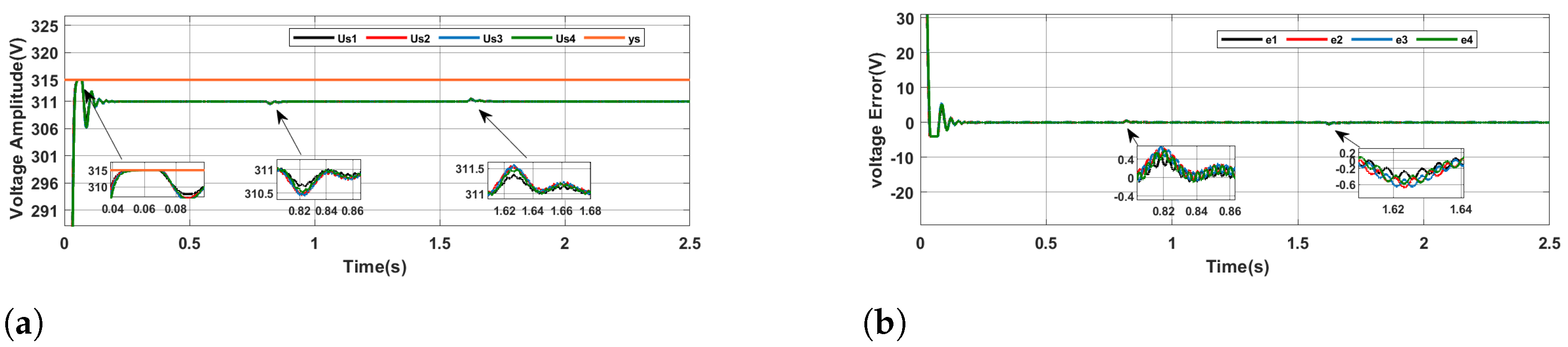
In this case, we applied the DAILC method to the test AC microgrid considering sensor saturation. As shown in Figure 4, despite not accounting for sensor saturation and relying solely on input–output data, this method successfully restored the output voltage to the preset value of 311 V. In this case, the saturation threshold for the sensors was set at 315 V. In the case of sensor saturation, due to the limitations of the sensor’s measurement range, there is a deviation between the measured value of the output voltage and its actual value. It can be observed from Figure 4 that during the transient processes in the AC microgrid, the peak of the output voltage was limited by the saturation threshold of 315 V. After processing with the DAILC, the output voltage eventually stabilized at the set value of 311 V, and the error converged to zero, thus verifying the effectiveness and practicality of the DAILC method.

4.2. DAILC Under Sensor Saturation and Variable Loads

In this case, we applied the DAILC method to the test AC microgrids considering both sensor saturation and variable load conditions. In microgrids, the unpredictability of load variations is primarily driven by the uncertainty of industrial production activities, fluctuations in commercial demand, changes in residential electricity usage habits, and variability in seasonal and weather conditions. Therefore, microgrids must possess excellent adaptability and rapid response capabilities to ensure the provision of stable and reliable power supply under various load demand scenarios. As shown in Figure 5, the saturation threshold of the sensor was set to 315 V, and load3 on the DG2 bus was added and removed at 0.8 s and 1.6 s, respectively. Observations from Figure 5 indicate that during the transient process of the microgrid, the peak output voltage was limited to the saturation threshold of 315 V. With the application of the DAILC method, even under changing load conditions, the output voltage quickly recovered to the preset value of 311 V, and the final error converged to zero. These results validate the effectiveness and practicality of the DAILC method in handling load variations.

4.3. DAILC Under Sensor Saturation and Topology Variations

In this case, we implemented the DAILC method on the test AC microgrid that was subject to both sensor saturation and topological changes. The specific topology changes are shown in Figure 6. The adaptability of microgrids to topological changes prominently demonstrates their plug-and-play characteristics. This feature not only enhances the flexibility and economic efficiency of the grid but also facilitates the broader integration of renewable energy sources and the implementation of grid automation. In the face of sudden increases in load or instability in energy output, the plug-and-play microgrid can quickly adjust its energy configuration, effectively ensuring the stability of the microgrid operation. As illustrated in Figure 7, the saturation threshold for the sensors was set to 315 V, and the DG4 was removed at 1 s. Observations from Figure 7 reveal that during the transient process of the microgrid, the peak output voltage was constrained by the saturation limit of 315 V. After applying the DAILC method, despite the topological changes, the output voltage quickly returned to the preset value of 311 V, and the final error converged to zero. These results demonstrate the effectiveness and practicality of the DAILC method in responding to topological changes.

To address the issue of communication network reliability, the results from this case serve to validate the robustness of the DAILC algorithm. Although the formal convergence proof in Section 3.3 assumes a strongly connected and time-invariant topology for mathematical tractability, the simulation results demonstrate that the algorithm possesses strong practical resilience. When a communication link fails, the topology is altered. As long as the remaining network remains connected (i.e., each node can still reach the virtual leader directly or indirectly), the local neighborhood error signals can continue to drive the system towards consensus, thereby ensuring voltage stability. Regarding communication delays, they have not been explicitly modeled in this paper. While the iterative learning nature of DAILC, which corrects errors in each cycle, may offer some inherent robustness to small, constant delays, a rigorous analysis of the impact of significant or time-varying delays remains a key topic for our future research.

4.4. Quantitative Performance Analysis and Discussion

To provide a rigorous statistical evaluation of the proposed DAILC method, we introduce several quantitative performance metrics as suggested: Root Mean Square Error (RMSE) for steady-state voltage tracking, convergence time after a disturbance, and robustness assessed by steady-state error fluctuation under measurement noise. We compare the performance of our DAILC method against a conventional distributed PI controller, which serves as a baseline. The results are summarized in

Table 3. Quantitative performance analysis.

Metric	Case	DAILC	PI
RMSE (V)	4.1: Sensor Saturation	0.08	0.25
	4.2: Variable Load	0.11	0.32
	4.3: Topology Change	0.09	0.28
Convergence Time (s)	4.2: Load Added	0.18	0.45
	4.3: DG4 Removed	0.21	0.52
Robustness under Noise (Error Fluctuation)		±0.15 V	±0.40 V
RMSE (95% CI)	Case 4.1 (20 runs)	[0.076, 0.084]	[0.241, 0.259]

.

The quantitative analysis, summarized in Table 3, reveals the superior performance of the DAILC method across several key metrics. Regarding tracking accuracy, the DAILC method consistently achieves a significantly lower Root Mean Square Error (RMSE)—0.08 V, 0.11 V, and 0.09 V across the three scenarios—compared to the PI controller’s 0.25 V, 0.32 V, and 0.28 V. In terms of transient performance, the DAILC method also excels in convergence time, which measures the duration for the system voltage to settle within a ±0.5% tolerance band of the reference after a major disturbance. In Case 4.2 and Case 4.3, the DAILC method’s convergence times of 0.18 s and 0.21 s are more than twice as fast as the PI controller, highlighting its superior adaptive response. Moreover, the DAILC’s robustness against noise was demonstrated by its ability to maintain a steady-state error fluctuation range of only ±0.15 V when white Gaussian noise was injected, whereas the PI controller exhibited larger fluctuations of ±0.40 V. Finally, to confirm the statistical significance of these findings, 20 Monte Carlo runs for Case 4.1 established a tight 95% confidence interval (CI) of [0.076, 0.084] for the DAILC method’s RMSE, which is distinctly separate from the PI controller’s CI of [0.241, 0.259], thereby validating that its superior performance is statistically significant. The proposed DAILC method is demonstrably superior to conventional PI control in terms of accuracy, speed, and robustness.

To address the crucial question of scalability, we analyze the communication and computational demands of the DAILC algorithm when applied to larger systems (e.g., 20+ DREGUs). The algorithm’s distributed nature is key to its scalability. The communication burden on an individual DREGU is determined by its number of direct neighbors (the node’s degree in graph G), not the total number of DREGUs (N) in the microgrid. For instance, in a ring or line topology, each node only communicates with two neighbors, regardless of whether N is 4 or 40. This contrasts sharply with centralized approaches where communication traffic to a central controller scales with N. Furthermore, as highlighted in Remark 7, the computational load per DREGU is exceptionally low. The control law update (9) and PPD estimation (11) involve only a few scalar algebraic operations. The memory and processing requirements for each agent remain constant and independent of the overall system size. This inherent O(1) complexity per node ensures that the DAILC algorithm can be efficiently deployed on low-cost microcontrollers, making it highly scalable and practical for large, heterogeneous microgrids.

Furthermore, it is important to connect the theoretical convergence to a “small neighborhood,” as proven in Theorem 1, with its practical size. The size of the final error bound, given by ${lim}_{k\to \infty }\parallel \mathbf{e}(t+1,k)\parallel =P/(1-\rho )h_1$, is directly proportional to the term $h_1$, which encapsulates the magnitude of disturbances, including the sensor noise $w_i(t,k)$. This theoretical relationship implies that higher noise levels will lead to a larger steady-state voltage deviation. Our existing quantitative analysis provides a concrete example of this. The robustness test reported in Table 3 was conducted with a low-level white Gaussian noise, resulting in a practical error fluctuation of approximately ±0.15 V. This value represents the practical size of the convergence neighborhood under typical, low-noise conditions. While the size of this neighborhood would increase with higher noise levels, the adaptive mechanism of the DAILC is designed to actively suppress these disturbances, ensuring the deviation remains within a small and acceptable range, thereby validating the practical robustness of our approach.

Beyond the PI controller, it is crucial to position our DAILC method relative to other advanced control strategies. Approaches like feedback linearization [17] and finite-time control [21] offer high performance but fundamentally rely on accurate system models. In real-world microgrids with high penetration of diverse and plug-and-play renewable sources, obtaining precise models is often impractical. Our DAILC method circumvents this challenge by being entirely data-driven, thus offering greater robustness to parameter uncertainties and system heterogeneity. Techniques using neural networks [26] or deep reinforcement learning [27] also handle nonlinearities well. However, they typically require extensive offline training datasets, significant computational resources for the training process, and their “black-box” nature can make stability verification challenging. In contrast, our DAILC is an online adaptive method that is computationally lighter and comes with a formal proof of convergence, making it more suitable for real-time implementation with lower-cost hardware. In conclusion, the DAILC method strikes a balance between performance, robustness, and implementation simplicity. It avoids the rigid model dependency of classical methods and the heavy computational/data requirements of complex AI techniques, positioning it as a practical and effective solution for modern, heterogeneous AC microgrids.

5. Conclusions

This paper introduces a model-free distributed data-driven adaptive iterative learning secondary voltage control method. Initially, utilizing input–output data from DREGUs, a time-variant linear data model that does not depend on specific microgrid system information is established. Subsequently, in response to measurement disturbances and sensor saturation, the DAILC algorithm is designed to achieve data-based adaptive restoration of voltage to reference values. Finally, we experimentally verify the convergence of this algorithm under conditions of sensor saturation and disturbances, confirming its effectiveness in restoring the secondary voltage of AC microgrids.

Although the test system is a standard benchmark that reflects realistic conditions, physical experimental validation is necessary to fully confirm the algorithm’s performance and robustness in real-world applications. Future research will focus on two main directions. First, we plan to implement and test the proposed DAILC algorithm on a hardware-in-the-loop (HIL) platform or a laboratory-scale microgrid to validate its practical feasibility. Second, this paper is limited to the study of voltage restoration to reference values. Therefore, future research will consider integrating reactive power sharing with secondary voltage regulation, addressing this issue comprehensively through a data-driven approach.