Drag Reduction in Compressible Channel Turbulence with Periodic Interval Blowing and Suction

Abstract

This paper employs direct numerical simulation (DNS) to investigate the influence of blowing and suction control on the compressible fully developed turbulent flow within an infinitely long channel. The spanwise blowing strips are positioned at uniform intervals along the bottom wall of the channel, while the suction strips are symmetrically placed on the top wall. The basic flow (uncontrolled case) and the controlled cases involving global control and interval control are compared at $Ma=0.8$ and 1.5. Although the wall mass flow rate remains constant across all controlled cases, the applied blowing/suction intensity and spanwise strip areas exhibit significant variations. The numerical results indicate that augmenting the blowing/suction intensity will alter the velocity gradient of the viscous sublayer in the controlled region. Nonetheless, a reduction in the area of the controlled region diminishes the impact of blowing/suction on drag reduction on the entire wall. The spatially averaged velocity profiles on the wall for cases with identical wall mass flow rates are nearly indistinguishable, suggesting that the wall mass flow rate is the primary factor influencing the spatially averaged drag reduction rate on the entire wall, rather than the blowing/suction intensity or the injected energy. This is because the wall mass flow rate influences the average peak position of the Reynolds stress, which, in turn, affects the skin friction drag. An increase in the wall mass flow rate correlates with a heightened drag reduction rate on the blowing side, while simultaneously leading to a rising drag increase rate on the suction side.

1. Introduction

Minimizing aerodynamic drag significantly enhances the performance and efficiency of contemporary high-speed aircraft. It is reported that a 1% reduction in drag results in at least a 0.75% reduction in fuel consumption and a reduction of roughly 2~3 tonnes CO₂ emission per flight [1]. Studies showed that friction drag constitutes approximately 50% of the total drag, and a 40% reduction in viscous drag is roughly equivalent to a 15% reduction in total drag [2,3]. Hence, reducing friction drag exhibits significant application prospects and research value for flow-control technologies.

Blowing/suction control, a prevalent active control technique, has emerged as a significant focus in flow-control research [4]. In contrast to passive control technologies like riblet control [5,6], blow/suction control can be dynamically modified in real time based on the flow field conditions to achieve optimal control efficacy. In comparison to active control technologies like energy deposition [7,8], it can attain a substantial drag reduction effect at a comparatively small energy cost. Blowing control infuses high-energy fluids into the boundary layer, and simultaneously modifies the velocity gradient of the viscous sublayer, thereby reducing skin friction drag. Additionally, suction control can also reduce drag by removing low-energy fluids from the boundary layer. However, suction control sometimes demonstrates a contrary effect to blowing control. Kametani and Fukagata [9] applied direct numerical simulation (DNS) to incompressible spatially developed turbulence at Reynolds number $R{e}_{\mathsf{\theta }}=3000$ based on the boundary layer thickness. The result confirmed that uniform blowing reduces the skin friction and uniform suction increases it. Additionally, turbulent fluctuations are enhanced by blowing and suppressed by suction. The FIK identity revealed that the mean convection term plays an important role in the drag reduction/augment due to blowing/suction. Kametani et al. [10] examined the control effect exerted by blowing and suction at Reynolds number $R{e}_{\mathrm{b}}=3000$ based on the bulk velocity and Mach number $Ma=0.8, 1.5$. The findings showed that the drag reduction rate (DRR) is affected by the blowing/suction amplitude instead of the Mach number. On the contrary, the control gain rises with the growing Mach number due to increasing density near the wall. Huang et al. [11] conducted an investigation on the drag reduction in the turbulent channel at $R{e}_{\mathrm{b}}=2800$. The spanwise traveling wave generated by wall blowing and suction is used to simulate wall oscillation. The study achieved a drag reduction of 24% with the mechanism of drag reduction closely linked to pressure–strain correlations. The opposition control effect of the turbulent channel at $R{e}_{\mathrm{b}}=3000$ was examined by Yao and Hussain [12] at bulk Mach number $M{a}_{\mathrm{b}}=0.3,0.8,1.5$. The sensing plane location $y_{\mathrm{d}}^{+}$ shifted from $y_{\mathrm{d}}^{+}=12.5$ for $M{a}_{\mathrm{b}}=0.3$ to $y_{\mathrm{d}}^{+}=20$ for $M{a}_{\mathrm{b}}=1.5$, which corresponds to the upward shift of the Reynolds stress peaks. Niu et al. [13] investigated the incompressible channel turbulence at $R{e}_{\mathrm{b}}=3000$ with various blowing/suction coefficients on the bottom/top wall. The drag reduction rate increased with the blowing coefficient. Nevertheless, drag reduction was achieved when the suction coefficient was 0.01, and the friction drag increased with the suction coefficient. Okochi et al. [14] investigated the drag reduction effects of opposition control and uniform blowing/suction on turbulent flow in a channel with a bump on the lower wall at $R{e}_{\mathrm{b}}=5600$ and 12,600. Opposition control can diminish friction drag, but has limited efficacy in reducing pressure drag. Uniform blowing reduces friction drag and pressure drag on the lower wall, but uniform suction amplifies friction drag on the upper wall. The disparity arises from the divergence in the two control mechanisms. Opposition control facilitates flow separation behind the bump, whereas uniform blowing mitigates it.

According to the experiment by Kornilov and Boiko [15,16], the skin friction will not immediately revert to its pre-control level after the cessation of control, but will gradually develop over a specified distance. The phenomenon is called the “memory effect” and it is inspiring for interval control. In comparison to global control, interval control arranges the controlled regions by intervals, hence diminishing energy expenditure for blowing and suction while preserving drag reduction and lowering the cost and complexity of installing the control device in engineering applications. Kametani et al. [17] studied the skin friction distribution in incompressible spatially developed turbulence. The skin friction diminished as the blowing was applied, and it recovered when the blowing stopped. The skin friction downstream of the controlled region was still lower than the uncontrolled case. Xie et al. [18] and Zeng et al. [19] explored the drag reduction of micro-hole blowing on a flat-plate turbulent boundary layer at $Ma=0.7$ and $Ma=2.25$, respectively, and reached similar conclusions. Lee et al. [20] employed four spanwise blowing strips at intervals in compressible channel turbulent flows at $R{e}_{\mathrm{b}}=3000$. The skin friction declined in the first few strips and rose in the last strip at $Ma=0.8$. However, the skin friction dropped in the non-blowing zones and recovered in the blowing zones at $Ma=1.5$. Hirokawa et al. [21] and Miura et al. [22] verified that the “memory effect” exists after blowing on the Clark-Y airfoil model. Furthermore, the “memory effect” has also been discovered in riblet [23,24] and porous media [25,26] control.

The design of interval control has great potential for drag reduction. Prior research has demonstrated that augmenting the blowing intensity by global blowing can enhance the drag reduction rate [9]. Nonetheless, in the context of interval blowing, the blowing area also influences the drag reduction capability. There is a deficiency in the literature about the critical factor that impacts the drag reduction rate for interval blowing. Our previous study [20] showed that interval blowing can diminish friction drag. However, we have not performed a comprehensive examination of how blowing area and blowing intensity influence the drag reduction effect. In this paper, a physical model of fully developed turbulence in a channel with infinite streamwise length is studied, the key factor that affects the drag reduction rate is explored, and the drag reduction effect of interval blowing and suction is analyzed. The paper is organized as follows: Section 1 introduces the research progress in blowing and suction control. Section 2 presents the physical model and the details of the computational codes. Section 3 clarifies the drag reduction effect of the interval control and analyzes the mechanism. Finally, Section 4 summarizes the main conclusions of this paper.

2. Computational Details

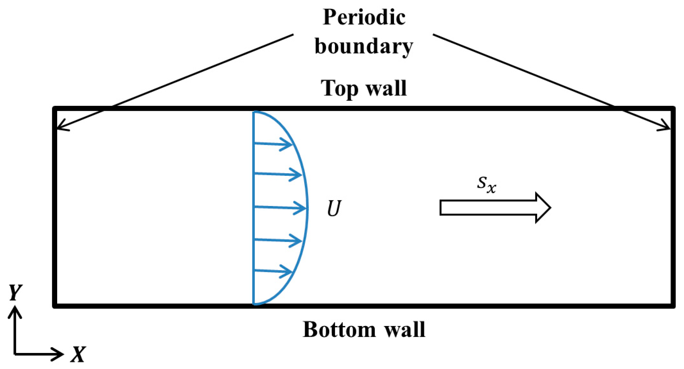
2.1. DNS Method and Physical Model

The governing equations of the numerical simulation are the compressible N-S equations. Hereafter, the variables with asterisk superscripts are dimensional quantities, and the variables without asterisks are dimensionless quantities. $\rho$, $u$, $v$, $w$, $T$, and $p$ are used to represent the density, the streamwise velocity, the normal velocity, the spanwise velocity, the temperature, and the pressure, respectively. The variables in the equations are non-dimensionalized using reference quantities such as the length $L^{\ast }$, the density ${\rho }_{\infty }^{\ast }$, the velocity in the X direction $u_{\infty }^{\ast }$, the temperature $T_{\infty }^{\ast }$, and their combinations. The dimensionless NS equations can be expressed as follows:

$${\displaystyle \frac{\mathsf{\partial }\mathit{Q}}{\mathsf{\partial }t}}+{\displaystyle \frac{\mathsf{\partial }{\mathit{F}}_x\left(\mathit{Q}\right)}{\mathsf{\partial }x}}+{\displaystyle \frac{\mathsf{\partial }{\mathit{F}}_y\left(\mathit{Q}\right)}{\mathsf{\partial }y}}+{\displaystyle \frac{\mathsf{\partial }{\mathit{F}}_z\left(\mathit{Q}\right)}{\mathsf{\partial }\mathrm{z}}}={\displaystyle \frac{\mathsf{\partial }{\mathit{G}}_x\left(\mathit{Q}\right)}{\mathsf{\partial }x}}+{\displaystyle \frac{\mathsf{\partial }{\mathit{G}}_y\left(\mathit{Q}\right)}{\mathsf{\partial }y}}+{\displaystyle \frac{\mathsf{\partial }{\mathit{G}}_z\left(\mathit{Q}\right)}{\mathsf{\partial }z}}+\mathit{S}$$

(1)

where $\mathit{Q}$ is the conserved variable vector, $\mathit{F}\left(\mathit{Q}\right)$ is the inviscid flux vector, $\mathit{G}\left(\mathit{Q}\right)$ is the viscous flux vector, $\mathit{S}$ is the source term, and the subscripts x, y, and z denote the components of $\mathit{F}$ and $\mathit{G}$ in the streamwise (X), normal (Y), and spanwise (Z) directions, respectively. The components of $\mathit{Q}$, $\mathit{F}$, $\mathit{G}$, and $\mathit{S}$ are defined as follows:

$$\begin{gathered} \mathit{Q}=\left(\begin{array}{c}\rho \\ \rho u\\ \rho v\\ \rho w\\ E\end{array}\right), {\mathit{F}}_x\left(\mathit{Q}\right)=\left(\begin{array}{c}\rho u\\ \rho u^2+p\\ \rho uv\\ \rho uw\\ u\left(E+p\right)\end{array}\right), {\mathit{F}}_y\left(\mathit{Q}\right)=\left(\begin{array}{c}\rho v\\ \rho uv\\ \rho v^2+p\\ \rho vw\\ v\left(E+p\right)\end{array}\right), {\mathit{F}}_z\left(\mathit{Q}\right)=\left(\begin{array}{c}\rho w\\ \rho uw\\ \rho vw\\ \rho w^2+p\\ w\left(E+p\right)\end{array}\right), \\ {\mathit{G}}_x\left(\mathit{Q}\right)=\left(\begin{array}{c}0\\ {\tau }_{xx}\\ {\tau }_{xy}\\ {\tau }_{xz}\\ k{\displaystyle \frac{\mathsf{\partial }T}{\mathsf{\partial }x}}+u{\tau }_{xx}+v{\tau }_{xy}+w{\tau }_{xz}\end{array}\right), {\mathit{G}}_y\left(\mathit{Q}\right)=\left(\begin{array}{c}0\\ {\tau }_{xy}\\ {\tau }_{yy}\\ {\tau }_{yz}\\ k{\displaystyle \frac{\mathsf{\partial }T}{\mathsf{\partial }y}}+u{\tau }_{xy}+v{\tau }_{yy}+w{\tau }_{yz}\end{array}\right), \\ {\mathit{G}}_z\left(\mathit{Q}\right)=\left(\begin{array}{c}0\\ {\tau }_{xz}\\ {\tau }_{yz}\\ {\tau }_{zz}\\ k{\displaystyle \frac{\mathsf{\partial }T}{\mathsf{\partial }z}}+u{\tau }_{xz}+v{\tau }_{yz}+w{\tau }_{zz}\end{array}\right), \mathit{S}=\left(\begin{array}{c}0\\ \rho s_x\\ 0\\ 0\\ \rho u{s}_x\end{array}\right) \end{gathered}$$

(2)

where $E$, $s_x$, and $k$ represent the internal energy, the external body force, and the thermal conductivity. $\tau$ is the viscous stress tensor, and its subscripts denote the viscous stress in different directions.

Hoam-OpenCFD (Version 1.10.4), developed by Li et al. [27], is used in this paper, and the direct numerical simulation (DNS) method is applied in the computation. The software uses the finite difference method (FDM) to acquire detailed flow field information via high-precision numerical simulation. It is highly appropriate for the examination of mixing layers, wall-bounded turbulence, jet flows, homogeneous isotropic turbulence (HIT), and numerous intricate unsteady flows. The temporal term $\mathsf{\partial }\mathit{Q}/\mathsf{\partial }t$ is advanced using the third-order Runge–Kutta method with a TVD property, and the inviscid term $\mathsf{\partial }\mathit{F}\left(\mathit{Q}\right)/\mathsf{\partial }\mathit{x}$ and the viscous term $\mathsf{\partial }\mathit{G}\left(\mathit{Q}\right)/\mathsf{\partial }\mathit{x}$ ($\mathit{x}={\left(x,y,z\right)}^T$) are calculated using the seventh-order upwind difference and the sixth-order central difference, respectively. The flowchart for the DNS analysis is presented in Figure 1.

The physical model models the turbulence in an infinitely long channel and it is assumed to be fully developed. A periodic unit of the channel is selected as the computational domain, and is displayed in 2D form in Figure 2. Periodic boundary conditions are used in the streamwise and spanwise directions, and isothermal and no-slip boundary conditions are used on the top and bottom wall. Given that the flow state in the channel is periodic, this simplification enables the turbulence to attain a fully developed state with reduced computational resources. The periodic motion of the channel turbulence is driven by the external body force $s_x$. This force is an artificial virtual force introduced to prevent the pressure gradient from disrupting the compressible turbulence. With a given target flow rate $q_0$, $s_x$ will increase/decrease if the actual flow rate is inferior/superior to $q_0$. During the computation, $s_x$ is corrected at every time step until the turbulence reaches a fully developed state.

The lengths of the cuboid computational domain in three directions are $\left(L_x,L_y,L_z\right)=2\pi \times 2\times 2\pi$, and the grid number of these three directions are $\left(N_x,N_y,N_z\right)=128\times 150\times 128$. Uniform grids are used in the streamwise and spanwise directions, while the distribution of grids in the normal direction is controlled by the following hyperbolic tangent function:

$$y_j=\tanh \left({\displaystyle \frac{4\left(j-1\right)}{N_y-1}}-2\right)/\tanh \left(2\right),j=1,2,\dots ,N_y$$

(3)

where $y_j$ is the normal coordinate of the grids, and $j$ is the normal number of the grid. Hence, the set of grids is sparser in the centerline and densest near the wall ($y^{+}=0.2$). The scale of the first layer of grids at the wall satisfies $\Delta y_1^{+}\approx 0.4$. The superscript “+” suggests that the wall viscous scale ${\nu }_{\mathrm{w}}/u_{\tau }$ is used as the dimensionless parameter, where ${\nu }_{\mathrm{w}}$ represents the kinematic viscosity at the wall and the wall friction velocity $u_{\tau }$ is defined as $u_{\tau }=\sqrt{{\tau }_{\mathrm{w}}/\rho }$.

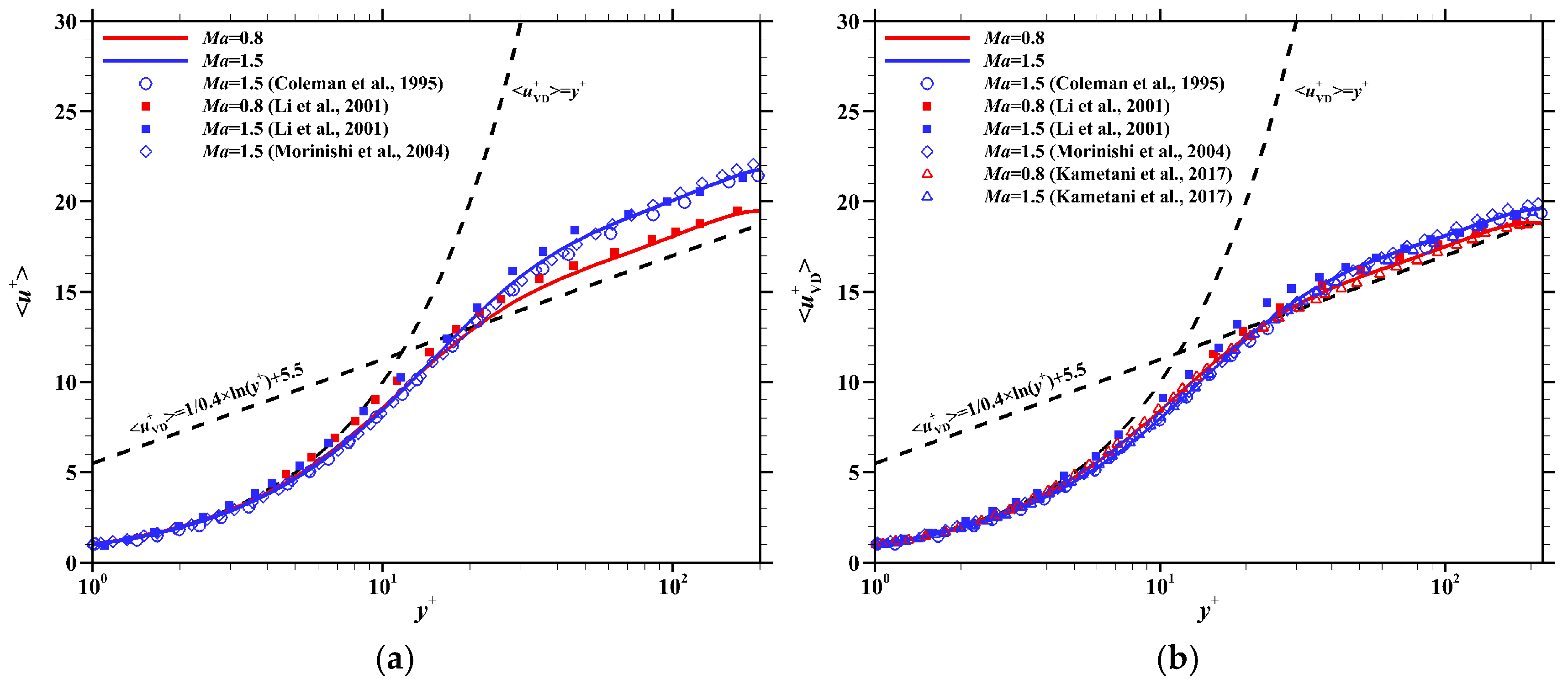
2.2. Basic Flow and Verification

Table 1. Computational settings for basic flow and relevant references.

Case	$\mathit{M}\mathit{a}$	$\mathit{R}{\mathit{e}}_{\mathit{b}}$	$\mathit{R}{\mathit{e}}_{\mathit{\tau }}$	${\mathit{L}}_{\mathit{x}}\times {\mathit{L}}_{\mathit{y}}\times {\mathit{L}}_{\mathit{z}}$	${\mathit{N}}_{\mathit{x}}\times {\mathit{N}}_{\mathit{y}}\times {\mathit{N}}_{\mathit{z}}$	$\Delta {\mathit{x}}_1^{+}\times \Delta {\mathit{y}}_1^{+}\times \Delta {\mathit{z}}_1^{+}$
Ma0.8	$0.8$	$3000$	$197$	$2\pi \delta \times 2\delta \times 2\pi \delta$	$128\times 150\times 128$	$9.8\times 0.40\times 9.8$
Ma1.5	$1.5$	$3000$	$220$	$2\pi \delta \times 2\delta \times 2\pi \delta$	$128\times 150\times 128$	$10.9\times 0.44\times 10.9$
Li et al. [28]	$0.8$	$3300$	$185$	$2\pi \delta \times 2\delta \times 2\pi \delta$	$101\times 140\times 101$	$11.6\times 0.40\times 11.6$
	$1.5$	$3300$	$185$	$2\pi \delta \times 2\delta \times 2\pi \delta$	$101\times 140\times 101$	$11.6\times 0.40\times 11.6$
Kametani et al. [10]	$0.8$	$3000$	$190$	$4\pi \delta \times 2\delta \times 4\pi \delta /3$	$256\times 120\times 128$	$9.32\times 0.22\times 6.22$
	$1.5$	$3000$	$220$	$4\pi \delta \times 2\delta \times 4\pi \delta /3$	$256\times 120\times 128$	$10.8\times 0.26\times 7.80$
Coleman et al. [29]	$1.5$	$3000$	$222$	$4\pi \delta \times 2\delta \times 4\pi \delta /3$	$144\times 119\times 80$	$19\times 0.1\times 12$
Morinishi et al. [30]	$1.5$	$3000$	$218$	$4\pi \delta \times 2\delta \times 4\pi \delta /3$	$120\times 180\times 120$	$23\times 0.36\times 7.6$

presents the computational settings of the basic flow (uncontrolled case) at $Ma=0.8$ and $Ma=1.5$. The half-width of the channel is $\delta =1$. The bulk density ${\rho }_{\mathrm{b}}$ and bulk velocity $U_{\mathrm{b}}$ in the channel are defined, respectively, as follows:

$${\rho }_{\mathrm{b}}={\displaystyle \frac{1}{2\delta }}{\displaystyle {\int }_0^{2\delta }〈\rho 〉dy}$$

(4)

$$U_{\mathrm{b}}={\displaystyle \frac{1}{2\delta ·{\rho }_{\mathrm{b}}}}{\displaystyle {\int }_0^{2\delta }〈\rho u〉dy}$$

(5)

For a certain variable $\phi$ in the flow field, $〈\phi 〉$ denotes the Reynolds average, and $\left\{\phi \right\}$ denotes the Favre average. The Favre average is defined as $\left\{\phi \right\}=〈\rho \phi 〉/〈\rho 〉$. The bulk Reynolds number $R{e}_{\mathrm{b}}$ and friction Reynolds number $R{e}_{\tau }$ are defined by $u_{\tau }$ and $U_{\mathrm{b}}$, respectively:

$$R{e}_{\mathrm{b}}={\displaystyle \frac{U_{\mathrm{b}}\delta }{\nu }}$$

(6)

$$R{e}_{\tau }={\displaystyle \frac{u_{\tau }\delta }{\nu }}$$

(7)

In this paper, the bulk Reynolds number is kept constant at $R{e}_{\mathrm{b}}=3000$, and the resultant friction Reynolds number is $R{e}_{\tau }=198$ at $Ma=0.8$ and $R{e}_{\tau }=220$ at $Ma=1.5$ with the same $s_x$.

In order to validate the computational codes and the settings, the computational results are compared with the relevant references [10,28,29,30]. The settings of the references are also listed in Table 1. Figure 3 provides the comparison of the velocity profile distribution for normalized average streamwise velocity $〈u^{+}〉$ and the Van Driest transformed velocity $〈u_{\mathrm{VD}}^{+}〉$. The Van Driest transformation helps mitigate the effect of compressibility when the Mach number is not very large, which can be expressed as follows:

$$<u_{\mathrm{VD}}^{+}>={\displaystyle {\int }_0^{<u^{+}>}\sqrt{\frac{〈\rho 〉}{{\rho }_{\mathrm{w}}}}}d<u^{+}>$$

(8)

In Figure 3a, though there is little difference from the literature [28] in the buffer layer due to a different $R{e}_{\mathrm{b}}$ and $R{e}_{\tau }$, the computational result shows good agreement with the literature [29,30] in the viscous sublayer and the logarithmic layer. In Figure 3b, the velocity profiles of $Ma=0.8$ and $Ma=1.5$ are very close to the empirical expression of the incompressible flow (black dashed line). The computational codes have been proven to be valid and effective and will be used for the subsequent computations.

3. Results and Discussions

3.1. Controlled Cases

The details of the cases with blowing/suction control are presented here. As illustrated in Figure 4, the controlled region and the uncontrolled region are staggered in the streamwise direction of the infinitely long channel. The blowing strips are implemented in the controlled region on the bottom wall and the suction strips are placed symmetrically on the top wall. A control unit is designated as the computational domain (blue dashed box), with the controlled region positioned centrally within this domain. The streamwise length of the controlled region is $L_{\mathrm{c}}$, and the area ratio of the controlled region and the computational domain $\alpha$ is defined as follows:

$$\alpha ={\displaystyle \frac{L_{\mathrm{c}}}{L_x}}$$

(9)

The control intensity $I$ is defined as follows:

$$I=\left\{\begin{array}{l}{\displaystyle \frac{v_{\mathrm{B}}}{u_{\infty }}} \left(\mathrm{blowing}\right)\\ {\displaystyle \frac{v_{\mathrm{S}}}{u_{\infty }}} \left(\mathrm{suction}\right)\end{array}\right.$$

(10)

In the controlled region, the wall-normal velocity $v_{\mathrm{w}}$ is adjusted to the $v_{\mathrm{B}}$ (blowing velocity) or $v_{\mathrm{S}}$ (suction velocity), while it is kept at zero in the uncontrolled region. The simulation employs velocity boundary conditions rather than modeling the real blowing/suction devices because this paper primarily investigates the impact mechanism of blowing/suction control on channel turbulence. This may lead to a specific discrepancy from the real-world conditions. However, owing to the small blowing/suction intensity, it can guarantee effective wall attachment performance for blowing/suction.

At each Mach number, one basic flow case and four controlled cases are calculated. C1 and C6 are the basic flow cases, C2 and C7 are the cases with global uniform blowing/suction, and the others are the interval blowing/suction cases with various $\alpha$. For controlled cases, the product of $I$ and $\alpha$ is an unchanged constant, so guaranteeing the control (blowing/suction) flow rate remains fixed in C2~C5 or C7~C10. The control effect parameters of these cases are listed in Table 2, where the subscript “B” represents the blowing side, “S” represents the suction side, and “0” represents the uncontrolled case. The drag reduction rate $DRR$ refers to the drag reduction/augment when it is positive/negative. The net energy-saving rate $S$ is determined by subtracting the loss of blowing power from the $DRR$. Furthermore, the control gain $G$ reflects the amplification effect of the blowing control on drag reduction. Their definitions [17] are expressed as follows:

$$C_{\mathrm{f}}={\displaystyle \frac{{\tau }_{\mathrm{w}}}{0.5{\rho }_{\mathrm{w}}{U}_{\mathrm{b}}^2}}$$

(11)

$$DR{R}_{\mathrm{B}/\mathrm{S}}={\displaystyle \frac{C_{\mathrm{f},0}-C_{\mathrm{f},\mathrm{B}/\mathrm{S}}}{C_{\mathrm{f},0}}}$$

(12)

$$DRR={\displaystyle \frac{DR{R}_{\mathrm{B}}+DR{R}_{\mathrm{S}}}{2}}$$

(13)

$$S={\displaystyle \frac{C_{\mathrm{f},0}-C_{\mathrm{f},\mathrm{B}/\mathrm{S}}-P_{\mathrm{B}}}{C_{\mathrm{f},0}}}$$

(14)

$$G={\displaystyle \frac{U_{\mathrm{b}}\left(C_{\mathrm{f},0}-C_{\mathrm{f},\mathrm{B}}\right)}{P_{\mathrm{B}}}}$$

(15)

where $P_{\mathrm{B}}$ is the input power of the blowing and is defined as

$$P_{\mathrm{B}}={\displaystyle \frac{1}{2}}\dot{m}{v}_{\mathrm{w}}^2\approx {\displaystyle \frac{\alpha 〈{\rho }_{\mathrm{w}}〉{〈v_{\mathrm{w}}〉}^3}{2}}$$

(16)

$\dot{m}$ is the wall mass flow rate, and $\dot{m}\propto \alpha ·I$.

Table 2. The control effect parameters of the basic flow and controlled cases.

Case Number	$\mathit{M}\mathit{a}$	$\mathit{I}$	$\mathit{\alpha }$	$\begin{array}{c}{\mathit{C}}_{\mathbf{f},\mathbf{B}}\end{array}$ (×10−2)	$\mathit{R}{\mathit{e}}_{\mathit{\tau },\mathbf{B}}$	$\begin{array}{c}\mathit{D}\mathit{R}{\mathit{R}}_{\mathbf{B}}\end{array}$ (%)	$\begin{array}{c}\mathit{D}\mathit{R}{\mathit{R}}_{\mathbf{S}}\end{array}$ (%)	$\begin{array}{c}\mathit{D}\mathit{R}\mathit{R}\end{array}$ (%)	$\begin{array}{c}\mathit{S}\end{array}$ (%)	$\begin{array}{c}\mathit{G}\end{array}$ (×104)
C1	0.8	0	×	1.14	197	×	×	×	×	×
C2	0.8	0.1%	1	0.99	184	12.7	−12.3	0.20	12.7	207.32
C3	0.8	0.2%	1/2	1.00	185	11.8	−14.3	−1.25	11.8	48.24
C4	0.8	0.3%	1/3	1.00	185	12.0	−13.9	−0.97	12.0	21.80
C5	0.8	0.5%	1/5	1.00	185	12.0	−13.2	−0.64	12.0	7.82
C6	1.5	0	×	0.98	220	×	×	×	×	×
C7	1.5	0.1%	1	0.85	205	13.7	−16.7	−1.51	13.7	152.66
C8	1.5	0.2%	1/2	0.84	203	15.1	−19.1	−2.01	15.1	41.99
C9	1.5	0.3%	1/3	0.84	203	15.1	−19.2	−2.08	15.1	18.60
C10	1.5	0.5%	1/5	0.84	203	14.7	−18.6	−1.93	14.7	6.52

Table 2. The control effect parameters of the basic flow and controlled cases.

Case Number	$\mathit{M}\mathit{a}$	$\mathit{I}$	$\mathit{\alpha }$	$\begin{array}{c}{\mathit{C}}_{\mathbf{f},\mathbf{B}}\end{array}$ (×10−2)	$\mathit{R}{\mathit{e}}_{\mathit{\tau },\mathbf{B}}$	$\begin{array}{c}\mathit{D}\mathit{R}{\mathit{R}}_{\mathbf{B}}\end{array}$ (%)	$\begin{array}{c}\mathit{D}\mathit{R}{\mathit{R}}_{\mathbf{S}}\end{array}$ (%)	$\begin{array}{c}\mathit{D}\mathit{R}\mathit{R}\end{array}$ (%)	$\begin{array}{c}\mathit{S}\end{array}$ (%)	$\begin{array}{c}\mathit{G}\end{array}$ (×104)
C1	0.8	0	×	1.14	197	×	×	×	×	×
C2	0.8	0.1%	1	0.99	184	12.7	−12.3	0.20	12.7	207.32
C3	0.8	0.2%	1/2	1.00	185	11.8	−14.3	−1.25	11.8	48.24
C4	0.8	0.3%	1/3	1.00	185	12.0	−13.9	−0.97	12.0	21.80
C5	0.8	0.5%	1/5	1.00	185	12.0	−13.2	−0.64	12.0	7.82
C6	1.5	0	×	0.98	220	×	×	×	×	×
C7	1.5	0.1%	1	0.85	205	13.7	−16.7	−1.51	13.7	152.66
C8	1.5	0.2%	1/2	0.84	203	15.1	−19.1	−2.01	15.1	41.99
C9	1.5	0.3%	1/3	0.84	203	15.1	−19.2	−2.08	15.1	18.60
C10	1.5	0.5%	1/5	0.84	203	14.7	−18.6	−1.93	14.7	6.52

According to the results from Kametani et al. [10] and Niu et al. [13], a larger blowing/suction velocity results in a higher/smaller $DRR$. Nonetheless, in the cases with interval control, the blowing area will also influence the control efficacy, which was not considered in the aforementioned work.

Because of the micro-blowing, the input power $P_{\mathrm{B}}$ is minimal; therefore, the net energy-saving rate $S$ is nearly equivalent to the $DR{R}_{\mathrm{B}}$ in all cases. It can also be concluded that, under the same control flow rate $\dot{m}$ (C2~C5 or C7~C10), $R{e}_{\tau ,\mathrm{b}}$, $DR{R}_{\mathrm{B}}$, $DR{R}_{\mathrm{S}}$, $DRR$, and $S$ are almost unchanged. This further indicates that it is the mass flow rate of the gas injected into the channel that affects the drag reduction rate of the periodic channel turbulence rather than the blowing/suction velocity or energy. This conclusion will be proved in the next section. The only distinction is the control gain $G$, which diminishes as the blowing intensity escalates.

The Mach number also influences the properties of drag reduction. With the same external body force $s_x$, $R{e}_{\tau ,\mathrm{B}}$ at $Ma=1.5$ is higher than that at $Ma=0.8$. Nevertheless, $C_{\mathrm{f},\mathrm{B}}$ is less at $Ma=1.5$ because $U_{\mathrm{b}}$ is enlarged at a higher Mach number. The drag reduction/augmentation effect on the blowing/suction side is more remarkable at a higher Mach number. Additionally, the control gain declines with the increasing Mach number due to the greater $U_{\mathrm{b}}$.

3.2. Effect of Injected Mass Flow Rate and Kinetic Energy

In order to further verify the dominant role of the injected mass flow rate in drag reduction,

Table 3. The control effect parameters of cases with higher mass flow rate (C2 and C7) and cases with larger injected kinetic energy (C11 and C12).

Case Number	$\mathit{M}\mathit{a}$	$\mathit{I}$	$\mathit{\alpha }$	$\begin{array}{c}{\mathit{C}}_{\mathbf{f},\mathbf{B}}\end{array}$ (×10−2)	$\mathit{R}{\mathit{e}}_{\mathit{\tau },\mathbf{B}}$	$\begin{array}{c}\mathit{D}\mathit{R}{\mathit{R}}_{\mathbf{B}}\end{array}$ (%)	$\begin{array}{c}\mathit{D}\mathit{R}{\mathit{R}}_{\mathbf{S}}\end{array}$ (%)	$\begin{array}{c}\mathit{D}\mathit{R}\mathit{R}\end{array}$ (%)	$\begin{array}{c}\mathit{S}\end{array}$ (%)	$\begin{array}{c}\mathit{G}\end{array}$ (×104)
C2	0.8	0.1%	1	0.99	184	12.7	−12.3	0.20	12.7	207.32
C11	0.8	0.4%	1/8	1.07	190	6.16	−6.11	0.02	6.16	12.57
C7	1.5	0.1%	1	0.85	205	13.7	−16.7	−1.51	13.7	152.66
C12	1.5	0.4%	1/8	0.91	211	7.28	−8.38	−0.55	7.28	10.09

gives a comparison of the supplementary cases C11 and C12 with C2 and C7 at $Ma=0.8$ and $Ma=1.5$, respectively. Global blowing/suction with a small I is implemented in C2 and C7, so they are chosen as the reference cases. Take C11 and C2 for example: the wall density ${\rho }_{\mathrm{w}}$ in both cases is 1.014. On the basis of Equation (16), the blowing velocity $v_{\mathrm{w}}$ in C11 is four times that in C2, but the blowing area in C11 is 1/8 of that in C2; hence, the injected kinetic energy in C11 is four times that in C2. As for the injected mass flow rate, owing to $\dot{m}\propto \alpha ·I$, $\dot{m}$ in C11 is half of that in C2. The settings of C11 guarantee that the wall mass flow rate of C2 is higher and the injection kinetic energy of C11 is greater. Apparently, the drag reduction rate ${DRR}_{\mathrm{B}}$ and the net energy-saving rate $S$ in C2 are almost twice that in C11, indicating that the drag reduction is strongly related to the injected mass flow rate instead of the injected kinetic energy. The result of $G$ reveals that the case with a greater mass flow rate has a higher control gain, but the average drag reduction rate shows little distinction. Table 2 illustrates that the wall mass flow rates in C2~C5 are the same, but the input power for C3, C4, and C5 is 4, 9, and 25 times more than that in C2, respectively. The drag reduction effect reveals that these four controlled cases are nearly identical, with a minimal difference between ${DRR}_{\mathrm{B}}$ and $S$, suggesting that the injected kinetic energy variation in these cases is negligible relative to the drag reduction impact. This reiterates that the wall mass flow rate is the critical determinant for the micro-blowing/suction control effect. A similar conclusion is also found in C7 and C12 at $Ma=1.5$.

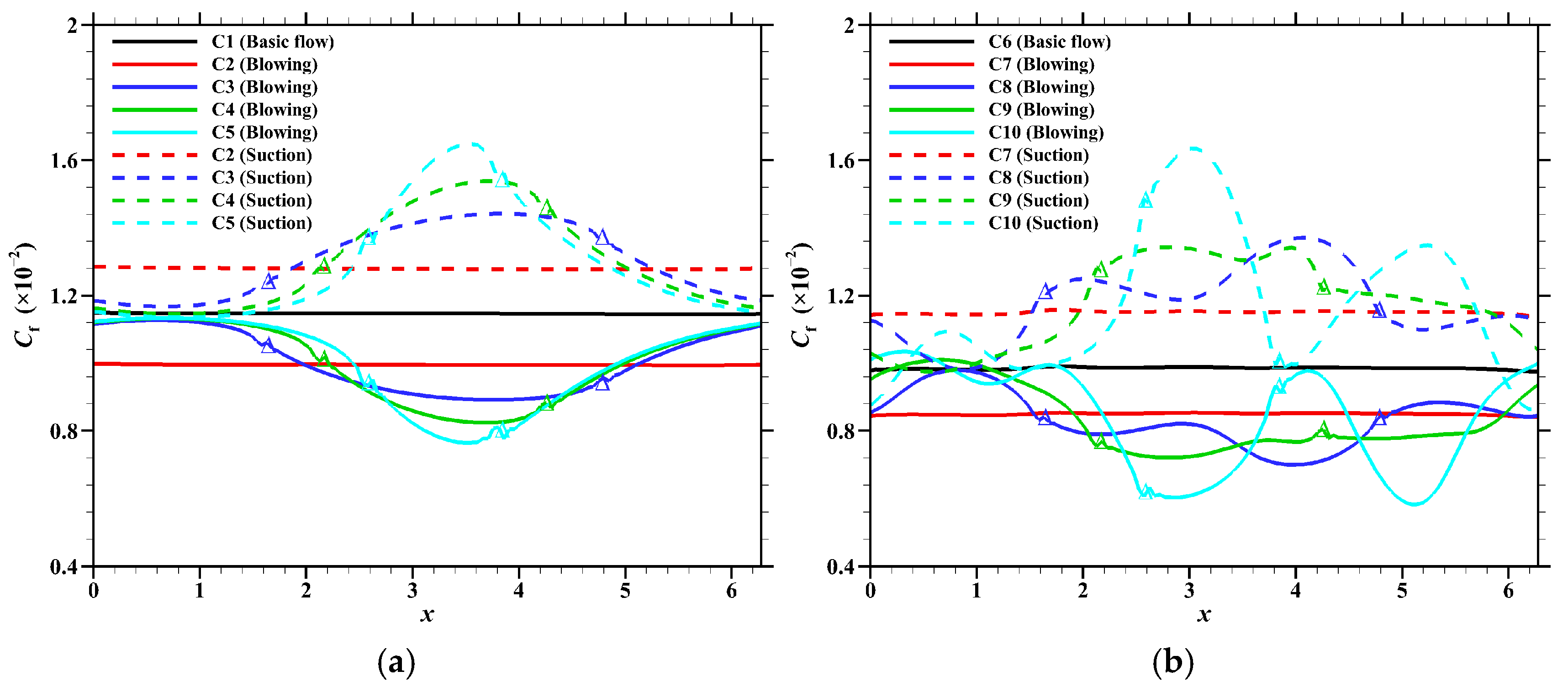
3.3. Skin Friction Distribution

Figure 5 depicts the skin friction coefficient distribution at $Ma=0.8$ and $Ma=1.5$. In contrast to global control, the skin friction coefficient $C_{\mathrm{f}}$ in the cases with interval control varies along the streamwise direction on account of the staggered arrangement of the controlled region and the uncontrolled region. In Figure 5a, the $C_{\mathrm{f}}$ curves of C3~C5 begin to decline/rise before the blowing/suction region, and the $C_{\mathrm{f}}$ value at the control starting position in C5 exhibits the greatest disparity from that of the basic flow. In the controlled region, the $C_{\mathrm{f}}$ curves reach the valley/peak and then recover. At the end point of the controlled region, the $C_{\mathrm{f}}$ value is lower than that at the start position on the suction side and higher on the blowing side. The valley/peak value of $C_{\mathrm{f}}$ in C5 is the lowest/highest because of the greatest blowing/suction intensity. The $C_{\mathrm{f}}$ curves on the blowing side and the suction side are roughly symmetrical about the basic flow curve.

In Figure 5b, the distribution of the skin friction coefficient becomes complicated at the supersonic speed. Oscillation is found after the control starting position. The $C_{\mathrm{f}}$ values at the control starting point and the end point are almost equivalent in C8 and C9. However, as the $L_{\mathrm{c}}$ shrinks to $L_x/5$ in C5, the $C_{\mathrm{f}}$ value at the end point is much greater than that at the control starting point on the blowing side, and lesser on the suction side. The valley/peak of the $C_{\mathrm{f}}$ curves shows asymmetry in C5, and the effect of suction is stronger than blowing. This phenomenon is different from the subsonic cases.

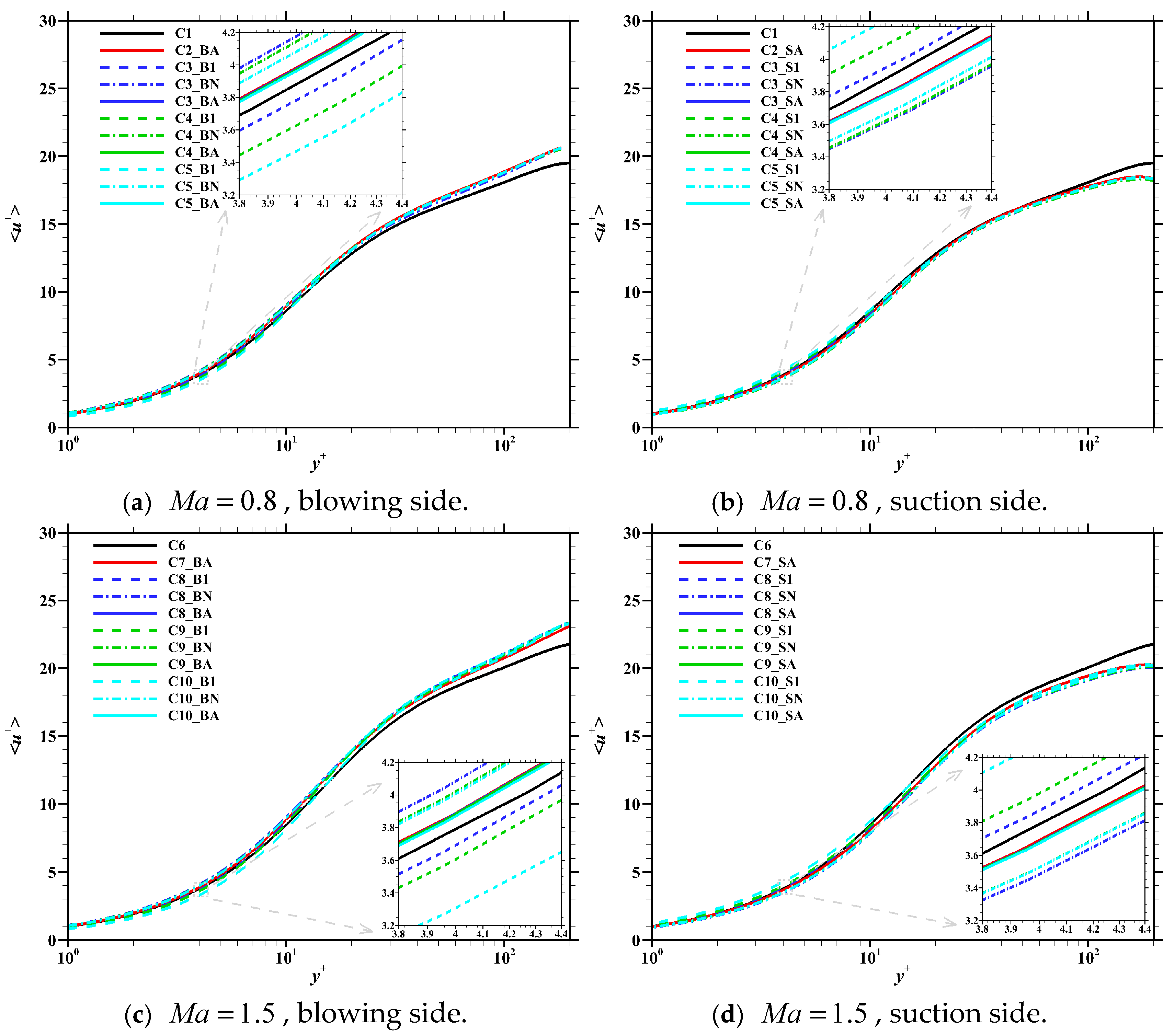
3.4. Averaged Velocity Profile

Figure 6 displays the spatially averaged velocity profile of the basic flow and the controlled cases in different regions, and the subfigures amplify the details in the viscous sublayer ($3.8\le y^{+}\le 4.4$). As shown in Figure 6a, in the viscous sublayer, the spatially averaged velocity on the top wall in C2~C5 almost coincides, and it is higher than the basic flow. As for C3~C5, the velocity gradient in the blowing region exceeds that basic flow, while the velocity gradient in the uncontrolled region is less than the basic flow. As the blowing intensity augments, the streamwise velocity in the blowing region lessens, with the reduction of the velocity gradient in the adjacent uncontrolled region. Nonetheless, the reduction in $L_{\mathrm{c}}$ from C2 to C5 results in a nearly consistent spatially averaged velocity gradient on the bottom wall in C2~C5. In Figure 6b, the velocity gradient in C2~C5 in the suction region exceeds the basic flow, whereas the velocity gradient in the uncontrolled region is below the basic flow level. As the blowing intensity increases, the velocity gradient rises in the suction region and uncontrolled region. This change is more distinct in the suction region. In Figure 6c,d, the tendency of the velocity profile in the viscous sublayer at $Ma=1.5$ is similar to that at $Ma=0.8$. At the supersonic speed, the variation in velocity gradient caused by the various blowing/suction intensity as well as the controlled area exhibits a more pronounced effect within the controlled region while remaining less significant in the uncontrolled region.

The above results indicate that blowing thickens the viscous sublayer and decrease the velocity gradient in the controlled region, with a more pronounced effect observed as blowing intensity increases. The viscous sublayer progressively diminishes in the uncontrolled region, with its thickness falling below that of the basic flow. Nonetheless, the “memory effect” of blowing exists, and the viscous sublayer remains thicker compared to cases with high blowing intensity in the uncontrolled region. If the wall mass flow rate remains constant (i.e., the product of α and I is invariant), the spatially averaged thickness of the viscous sublayer and the velocity gradient on the entire wall will be identical. This is due to the fact that, while the viscous sublayer is thicker in cases with high blowing intensity, a reduction in the blowing area $\alpha$ results in the controlled region with a smaller velocity gradient having a lesser impact on the spatially averaged value on the entire wall. The effect of suction is contrary to that of blowing, yet similar conclusions are drawn.

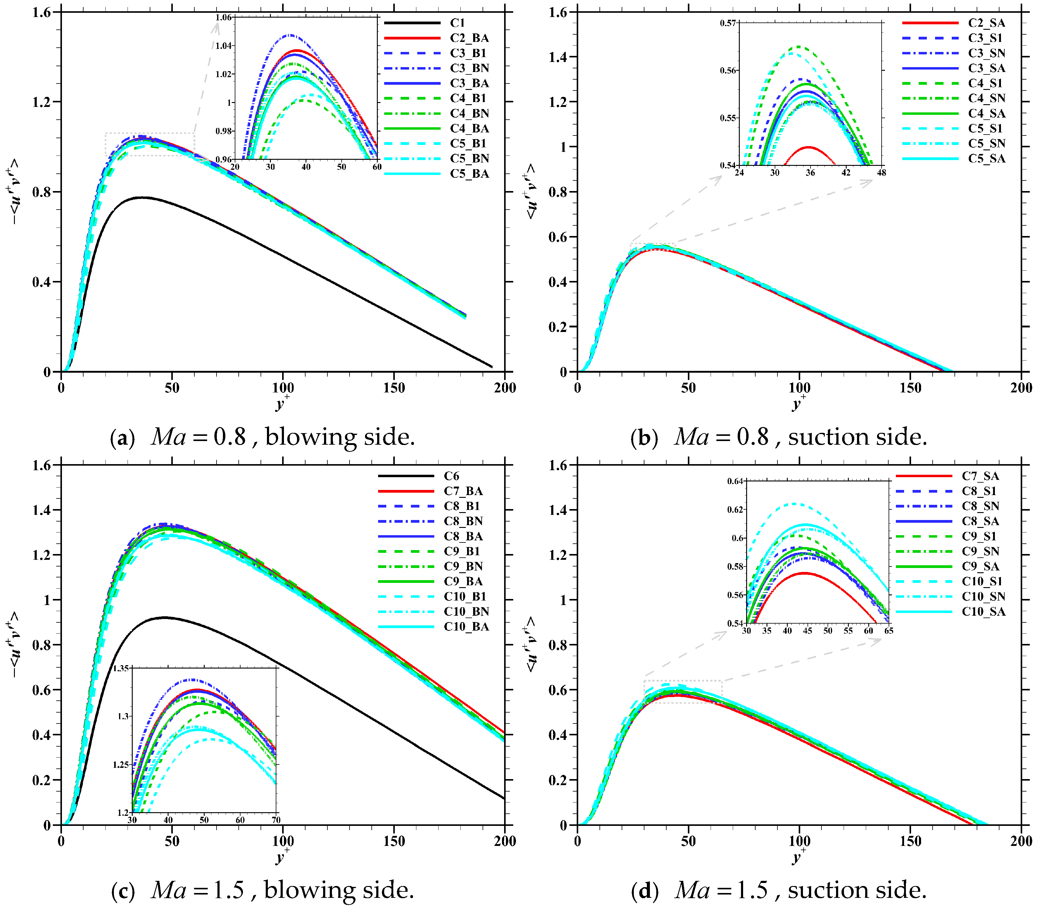
3.5. Reynolds Stress

The Reynolds normal stress (RNS) $〈u^{\prime +}{u}^{\prime +}〉$ and the Reynolds shear stress (RSS) $〈u^{\prime +}{v}^{\prime +}〉$ can reflect the turbulence intensity. Figure 7 presents the Reynolds normal stress on the blowing/suction side at various Mach numbers. The Reynolds stress on the blowing/suction side is normalized by the spatially averaged wall friction velocity on the bottom/top wall, respectively. Comparing Figure 7a,c, the RNS peak on the blowing side in C2~C5 is higher than the basic flow, which is consistent with the aforementioned literature [10]. Furthermore, the RNS peak is at $y^{+}\approx 15$ for $Ma=0.8$ and $y^{+}\approx 20$ for $Ma=1.5$. The wall-normal height of the RNS peak increases with the blowing intensity, but the distinction is not readily apparent at the same Mach number. The RNS peak in the blowing region is lower than that in the uncontrolled region, and this discrepancy also expands with the blowing intensity. In Figure 7a, the RNS peak is the highest in C2 at $Ma=0.8$, followed by C4, C3, and C5. This reveals that the spatially averaged RNS peak on the bottom wall declines as the $\mathsf{\alpha }$ decreases generally, but it rebounds when $\mathsf{\alpha }=1/3$. In Figure 7c, the relationship between the RNS peak and $\mathsf{\alpha }$ becomes unclear at $Ma=1.5$.

On the contrary, the spatially averaged RNS peak on the suction side in C2~C5 is lower than the basic flow, as shown in Figure 7b,d. The spatially averaged RNS peak on the suction side is located at $y^{+}\approx 17$ for $Ma=0.8$ and $y^{+}\approx 22$ for $Ma=1.5$, which is slightly higher than the blowing side. In contrast to the blowing side, the wall-normal height of the RNS peak decreases with the suction intensity. Additionally, the spatially averaged RNS peak in the suction region exceeds that in the uncontrolled region. In Figure 7b, the RNS peak diminishes with the increasing $\mathsf{\alpha }$ at $Ma=0.8$, but it recovers and even exceeds that in C2 when $\mathsf{\alpha }=1/5$. In Figure 7d, the spatially averaged RNS peak on the suction side in C10 is still the highest, but the spatially averaged RNS peak in the suction region in C10 is inferior to that in C8. The suction intensity in C10 is significantly violent, resulting in a pronounced diminishing influence on the RNS peak.

Figure 8 depicts the spatially averaged Reynolds shear stress (RSS) on the blowing/suction side at various Mach numbers. Given that the RSS in the basic flow and on the blowing side of the controlled cases is negative, $-〈u^{\prime +}{v}^{\prime +}〉$ is designated as the ordinate variable in Figure 8a,c. The RSS peak is at $y^{+}\approx 37$ and $y^{+}\approx 48$ for $Ma=0.8$ and 1.5 on the blowing side, while $y^{+}\approx 35$ and $y^{+}\approx 44$ for $Ma=0.8$ and 1.5 on the suction side, respectively. In Figure 8a,c, the spatially averaged RSS peak on the bottom wall in C2~C5 and C7~C10 exceeds that of the basic flow. However, the spatially averaged RSS peak value within the blowing region is lower than that in the uncontrolled region. As the blowing intensity increases, the spatially averaged RSS peak in the blowing region rapidly declines, and the spatially averaged RSS peak on the wall also diminishes. In Figure 8b,d, the spatially averaged RSS peak on the top wall increases with the suction intensity in general. However, it is found that the RSS peak falls back in C5.

The results indicate that, with an increase in blowing intensity, the peak position of the Reynolds stress shifts upward. This suggests that the primary energy-containing structures in the buffer layer, including low-speed streaks and quasi-streamwise vortices (QSV), are influenced by blowing control and migrate away from the wall. Consequently, this weakens the ejection and sweep phenomena in the near-wall region, leading to a reduction in skin friction drag [13]. Upon entering the uncontrolled region, the peak position of Reynolds stress diminishes, and the energy-containing structures move closer to the wall once more, leading to a recovery of drag. Generally, when the wall mass flow rate remains constant, the spatially averaged peak position of the Reynolds stress on the entire wall shows minimal variation. This suggests that the wall mass flow rate influences the average peak position of the Reynolds stress, which, in turn, affects the skin friction drag. Suction control will lower the peak position of Reynolds stress and elevate the friction drag, yet the conclusion aligns closely with that of blowing control.

4. Conclusions

In this paper, direct numerical simulation (DNS) is employed on infinitely long compressible channel turbulence. The blowing strips are arranged intermittently on the bottom wall and the suction strips are assigned symmetrically on the top wall. A periodic unit is selected as the computational domain. In the controlled cases, the wall mass flow rate is kept constant at each Mach number. The main conclusions are summarized as follows:

(1)

The global drag reduction is strongly related to the wall mass flow rate, instead of the injected energy or blowing/suction intensity. Although the increasing blowing/suction intensity leads to a more significant control effect in the controlled region, the reduced controlled area will weaken the effect on the entire wall. In conclusion, when the Mach number and wall mass flow rate are identical, the velocity gradient within the viscous sublayer remains constant.

(2)

At the subsonic speed, the skin friction coefficient $C_{\mathrm{f}}$ increases in the blowing region and decreases in the suction region. The $C_{\mathrm{f}}$ variation in the controlled region rises with the blowing/suction intensity. At the supersonic speed, the $C_{\mathrm{f}}$ curve oscillates in the controlled region. Generally, $C_{\mathrm{f}}$ decreases in the blowing region and increases in the suction region, but this phenomenon becomes pronounced when the blowing/suction intensity reaches 0.5%.

(3)

In the controlled region, blowing will result in the peak position of the Reynolds stress shifting upward, whereas suction will cause the peak position to move closer to the wall. Within the controlled region, the variation in the peak position caused by blowing/suction will progressively diminish. When the wall mass flow rate is constant, the spatially averaged peak position of the Reynolds stress on the entire wall remains nearly the same.

The findings of this research may offer assistance and guidance for engineering applications, including long-distance pipeline transport of high-velocity gas or engine intake ducts. To minimize friction drag, it is essential to maximize the wall mass flow rate of the blowing control. If the wall mass flow rate is fixed, global blowing is recommended, or the blowing area should be expanded, which can diminish the blowing intensity and thus lower the necessary input power for blowing and enhance the control gain.

References

1. Ricco, P.; Skote, M.; Leschziner, M.A. A review of turbulent skin-friction drag reduction by near-wall transverse forcing. Prog. Aerosp. Sci. 2021, 123, 100713. [Google Scholar] [CrossRef]
2. Kornilov, V. Combined blowing/suction flow control on low-speed airfoils. Flow Turbul. Combust. 2021, 106, 81–108. [Google Scholar] [CrossRef]
3. Abbas, A.; De Vicente, J.; Valero, E. Aerodynamic technologies to improve aircraft performance. Aerosp. Sci. Technol. 2013, 28, 100–132. [Google Scholar] [CrossRef]
4. Aabid, A.; Khan, S.A.; Baig, M. A critical review of supersonic flow control for high-speed applications. Appl. Sci. 2021, 11, 6899. [Google Scholar] [CrossRef]
5. Mele, B. Riblet drag reduction modeling and simulation. Fluids 2022, 7, 249. [Google Scholar] [CrossRef]
6. Pakatchian, M.R.; Rocha, J.; Li, L. Advances in riblets design. Appl. Sci. 2023, 13, 10893. [Google Scholar] [CrossRef]
7. Kumar, S.; Kulkarni, V. An effective means of drag reduction in high enthalpy flow through unsteady energy deposition. Acta Astronaut. 2021, 186, 533–543. [Google Scholar] [CrossRef]
8. Knight, D.; Kianvashrad, N. Review of energy deposition for high-speed flow control. Energies 2022, 15, 9645. [Google Scholar] [CrossRef]
9. Kametani, Y.; Fukagata, K. Direct numerical simulation of spatially developing turbulent boundary layers with uniform blowing or suction. J. Fluid Mech. 2011, 681, 154–172. [Google Scholar] [CrossRef]
10. Kametani, Y.; Kotake, A.; Fukagata, K.; Tokugawa, N. Drag reduction capability of uniform blowing in supersonic wall-bounded turbulent flows. Phys. Rev. Fluids 2017, 2, 123904. [Google Scholar] [CrossRef]
11. Huang, Y.; Wang, L.; Fu, S. Drag reduction in turbulent channel flows by a spanwise traveling wave of wall blowing and suction. Phys. Fluids 2021, 33, 095111. [Google Scholar] [CrossRef]
12. Yao, J.; Hussain, F. Drag reduction via opposition control in a compressible turbulent channel. Phys. Rev. Fluids 2021, 6, 114602. [Google Scholar] [CrossRef]
13. Niu, J.; Wang, J.; Liu, X.; Gong, J.; Dong, L. Micro-suction and micro-blowing on channel flow: Large eddy simulation of velocity normalization, root-mean-square velocity fluctuations, and Reynolds stress. Int. J. Green Energy 2025, 1–18. [Google Scholar] [CrossRef]
14. Okochi, Y.; Nabae, Y.; Fukagata, K. Direct numerical simulations of a bump-installed turbulent channel flow for drag reduction by blowing and suction. J. Fluid Mech. 2025, 1010, A69. [Google Scholar] [CrossRef]
15. Kornilov, V.I.; Boiko, A.V. Efficiency of air microblowing through microperforated wall for flat plate drag reduction. AIAA J. 2012, 50, 724–732. [Google Scholar] [CrossRef]
16. Kornilov, V.I.; Boiko, A.V. Flat-plate drag reduction with streamwise noncontinuous microblowing. AIAA J. 2014, 52, 93–103. [Google Scholar] [CrossRef]
17. Kametani, Y.; Fukagata, K.; Örlü, R.; Schlatter, P. Drag reduction in spatially developing turbulent boundary layers by spatially intermittent blowing at constant mass-flux. J. Turbul. 2016, 17, 913–929. [Google Scholar] [CrossRef]
18. Xie, L.; Zheng, Y.; Zhang, Y.; Ye, Z.; Zou, J. Effects of localized micro-blowing on a spatially developing flat turbulent boundary layer. Flow Turbul. Combust. 2020, 107, 51–79. [Google Scholar] [CrossRef]
19. Zeng, F.; Qiu, Y.; Jiang, Z.; Tong, C.; Hu, C.; Chen, W. Direct numerical simulation of skin friction drag reduction on supersonic turbulent boundary layers with micro-blowing. Phys. Fluids 2024, 36, 095165. [Google Scholar] [CrossRef]
20. Lee, S.; Zhang, Y.; Zhao, Y.; Luo, J.; Zheng, Y. Effects of interval blowing on drag reduction incompressible channel turbulent flows. Phys. Fluids 2025, 37, 045136. [Google Scholar] [CrossRef]
21. Hirokawa, S.; Ohashi, M.; Eto, K.; Fukagata, K.; Tokugawa, N. Turbulent friction drag reduction on Clark-Y airfoil by passive uniform blowing. AIAA J. 2020, 58, 4178–4180. [Google Scholar] [CrossRef]
22. Miura, S.; Ohashi, M.; Fukagata, K.; Tokugawa, N. Drag reduction by uniform blowing on the pressure surface of an airfoil. AIAA J. 2022, 60, 2241–2250. [Google Scholar] [CrossRef]
23. Al-Kayiem, H.H.; Lim, D.C.; Kurnia, J.C. Large eddy simulation of near-wall turbulent flow over streamlined riblet-structured surface for drag reduction in a rectangular channel. Therm. Sci. 2020, 24, 2793–2808. [Google Scholar] [CrossRef]
24. Sharma, V.; Dutta, S. Experimental and Numerical Investigation of Bio-Inspired Riblet for Drag Reduction. J. Fluids Eng. 2022, 145, 021207. [Google Scholar] [CrossRef]
25. Ma, R.; Gao, Z.H.; Lu, L.S.; Chen, S.S. Skin-friction drag reduction by local porous uniform blowing in spatially developing compressible turbulent boundary layers. Phys. Fluids 2022, 34, 125130. [Google Scholar] [CrossRef]
26. Kong, W.; Dong, H.; Wu, J.; Yang, L.; Gao, S. Control of frictional and total drag by porous media at high Reynolds number wall turbulence conditions. Phys. Fluids 2025, 37, 035205. [Google Scholar] [CrossRef]
27. Li, X.; Fu, D.; Ma, Y.; Liang, X. Direct numerical simulation of compressible turbulent flows. Acta Mech. Sin. 2010, 26, 795–806. [Google Scholar] [CrossRef]
28. Li, X.; Ma, Y.; Fu, D. DNS and scaling law analysis of compressible turbulent channel flow. Sci. China Ser. A Math. 2001, 44, 645–654. [Google Scholar] [CrossRef]
29. Coleman, G.N.; Kim, J.; Moser, R.D. A numerical study of turbulent supersonic isothermal-wall channel flow. J. Fluid Mech. 1995, 305, 159–183. [Google Scholar] [CrossRef]
30. Morinishi, Y.; Tamano, S.; Nakabayashi, K. Direct numerical simulation of compressible turbulent channel flow between adiabatic and isothermal walls. J. Fluid Mech. 2004, 502, 273–308. [Google Scholar] [CrossRef]
Figure 1. Flowchart of DNS analysis.
Applsci 15 07117 g001
Figure 2. Schematic diagram of the X-Y cross section of the computational domain.
Applsci 15 07117 g002
Figure 3. Velocity profile distribution for (a) u + and (b) u VD + of the basic flow [10,28,29,30].
Applsci 15 07117 g003
Figure 4. Schematic diagram of the top/bottom wall of the physical model. The blue dashed box represents the computational domain.
Applsci 15 07117 g004
Figure 5. Skin friction coefficient distribution along the streamwise direction at (a) M a = 0.8 and (b) M a = 1.5 . The delta symbols denote the start and end of the controlled region for each case with interval control.
Applsci 15 07117 g005
Figure 6. Spatially averaged velocity profile in different regions. BA: on the bottom wall; B1: in the blowing region; BN: in the uncontrolled region of the bottom wall; SA: on the top wall; S1: in the suction region; SN: in the uncontrolled region of the top wall.
Applsci 15 07117 g006
Figure 7. Spatially averaged Reynolds normal stress in different regions. The legend description is the same as Figure 6.
Applsci 15 07117 g007
Figure 8. Spatially averaged Reynolds shear stress in different regions. The legend description is the same as Figure 6.
Applsci 15 07117 g008