Semi-Supervised Anomaly Detection for the Identification of Damages in an Aerospace Sandwich Structure Based on Synthetically Generated Strain Data

Abstract

The structural health monitoring (SHM) of safety relevant composite components is becoming increasingly relevant as it enables in-service diagnosis and data acquisition capabilities, contributing to the optimization and efficient operation of the overall system and ultimately saving costs and resources. In this field, machine learning (ML) techniques are attracting growing attention due to their capability to recognize complex patterns, making them very suitable for the identification of damages in operating mechanical structures. However, the acquisition of sufficiently large amounts of labeled and representative data from both pristine and damaged structures is very costly. To address this, a ML-based SHM approach is proposed that identifies structural damage using only physics-based synthetic strain data generated from the structure’s numerical finite element model. It employs a semi-supervised anomaly detection approach, trained solely on synthetic pristine data, to identify deviations in experimental data indicating damage. The method is validated on an aircraft spoiler demonstrator made of a composite sandwich panel, instrumented with a strain gauge grid on its surface layer. The results show that the proposed SHM approach accurately classifies damaged and undamaged experimental data, independent of the prevailing load case, solely based on synthetic pristine strain data. It is also able to localize these damages in the form of a confidence area with respect to the sensor grid. This demonstrates the feasibility of using only synthetic pristine data for data-driven SHM of composite aerospace structures.

1. Introduction

The use of FRP (fiber-reinforced polymer) composite components in modern civil and military aircraft is steadily increasing. To give an example, currently, more than half of the components of the Boeing 787 and Airbus A350 XWB are composite parts [1]. They are employed due to their lightweight and high-strength properties, which in turn contributes to a lighter overall aircraft, improving fuel efficiency and reducing emissions. The advantages of composite components however come at the cost of higher complexity when compared to conventional metal components, requiring an increased focus on maintenance and inspection [1,2,3]. On the other hand, from an operational point of view, there is the need to reduce aircraft maintenance and down-times as much as possible. Structural health monitoring (SHM), in the sense of permanently installed sensor networks which enable in-service monitoring of aircraft structures [4], presents a promising approach for ensuring the safety, reliability, and longevity of such structures. It further enables the efficient operation of components, ultimately saving costs and resources, e.g., through optimized maintenance strategies. SHM systems can be divided into four main levels regarding their capability: Level 1—Detection of the existence of damage; Level 2—Localization of the position of damage; Level 3—quantification of the extent of damage; Level 4—classification of the damage type; and Level 5—assessment of the structures integrity [5]. When focusing on the various methods currently used in SHM applications, Güemes et al. [6] summarizes them as vibration methods [7], guided waves [8], acoustic emission [9] and strain-based methods [1]. Out of these, strain-based methods are particularly interesting, where cost efficient and robust strain gauges are applied to or embedded into the surface of a structure to measure the deformation experienced under various loads [10]. A popular example is the structural health and usage monitoring system of the Eurofighter Typhoon aircraft, which utilizes the data of strain gauges [11]. More recent strain-based SHM systems make use of fiber optical sensors (FOSs), particularly those based on fiber Bragg gratings (FBG) [1]. They are particularly interesting for the monitoring of composite parts as they can be embedded into the structure. By providing multi-point measurements along the fiber, FBG sensors allow the monitoring of a large area [3].

Parallel to this, rapidly advancing machine learning (ML) techniques are increasingly applied, promising to further enhance the capabilities and application of SHM methods [4]. ML techniques, particularly those designed for pattern recognition and anomaly detection, are well-suited for interpreting the large and often noisy datasets generated in SHM. These methods can automate and optimize the detection of structural damages by learning complex relationships within the data. Kesavan et al. [12,13] propose a machine learning-based health monitoring approach that utilizes discrete strain measurements as health indicators. Their work introduces a novel data-driven methodology for detecting debonding using an artificial neural network (ANN). The approach analyzes the strain distribution within the structure and employs the ANN to predict the location and size of the disbond, independent of the magnitude and direction of the applied load. Teimouri et al. [14] developed an artificial neural network-based SHM system to detect and quantify delaminations in composite airfoils using simulated strain data. Their approach demonstrated an accurate prediction of damage size and location, highlighting the potential of ANN models for real-time structural assessment under manufacturing uncertainties. Lin et al. [15] demonstrated the use of convolutional neural networks (CNNs) trained on simulated strain data from a digital twin of an aircraft composite wing to detect and localize damage with high accuracy, even under noisy conditions. Lee et al. [16] introduced a deep autoencoder-based method to detect and classify fatigue damage modes in carbon fiber-reinforced polymer (CFRP) laminates, relying solely on healthy-state data and clustering latent features for damage type differentiation. More advanced systems combine multiple data sources and learning methods. Sun et al. [17,18] applied deep learning techniques, specifically convolutional and recurrent neural networks, generative adversarial networks, and attention mechanisms, to recover missing strain data and predict pipeline deformation using long-gauge FBG sensors and multi-source monitoring.

However, the application of ML in SHM also introduces its own challenges. One of the primary difficulties is the requirement for large amounts of labeled data, which is essential for training supervised learning models [4]. Considering SHM, this data also needs to sufficiently represent the pristine and damaged states of the system, under a variety of loading conditions. Thus, any potential damage needs to have a measurable influence on the available data in some form. Moreover, to evaluate damage beyond detection and localization, data samples of the damaged structure must exist at the time of training. In the context of composite structures, often safety-critical or high performance parts, acquiring such data is particularly expensive and time-consuming [2].

When only focusing on the detection and localization of damages, one way to avoid the acquisition of damage data is to utilize anomaly detection ML approaches, which only require data of a pristine structure for the classification task. This was carried out by Grassia et al. [19] by developing a strain-based SHM method that uses ANN to learn the correlation between the strain at a given location to the strain at neighboring locations, where the measurements are provided by a sensor grid, applied on the surface of a plate-like structure. The method is trained on experimental data of the pristine structure and tested on data of the same structure but with introduced damage.

A further approach to address the data acquisition challenge is to use analytical or numerical models for the efficient generation of training data. Bergmayr et al. [20] developed a classifier, which was trained with pristine data and synthetically generated damage data, obtained from simulations of the numerical model of a structure. With this, the detection of damages in the strain data of the real structure was realized. Here as well, the relationship between strains at different locations was modeled by means of local bi-linear regressions, which are then evaluated by a random forest classifier.

The strain-based damage evaluation proposed in this work combines the above mentioned approaches, as it adopts the concept of detecting deviations from the learned relationship between individual strain values provided by a sensor grid and additionally utilizes an existing framework for the generation of physics-based strain data for the efficient generation of a large amount of training samples [21]. Furthermore, these samples are only required to describe the state of a pristine structure. Based on the numerical training samples, the SHM application shall identify damages in experimental data of the real structure by comparing new data against learned characteristics of the structure’s pristine state. This eliminates the need for expensive data representing the damaged structure. The described approach is also referred to as semi-supervised anomaly detection [22]. It is conceptually situated between supervised and unsupervised learning, since the model only sees samples which are known to be pristine at the training stage. Only during the monitoring stage do the input data potentially contain anomalous samples, which the model then ideally detects. A major challenge herein is the detection of an anomaly, regardless of the environmental and operational variations, e.g., different load cases or temperature changes [2,22]. The method is conclusively validated by applying it to an aircraft spoiler demonstrator, consisting of a composite sandwich panel, which is subjected to mechanical loading that imitates a typical aerodynamic loading scenario. The proposed approach demonstrates how spatially distributed strain sensing points on a structure can be leveraged by an ensemble of regression models to detect deviations from normal behavior using only numerical data of the pristine structure. By relying exclusively on the relationships between strain signals in the undamaged state, the method eliminates the need for labeled damage data. Furthermore, by leveraging an existing framework for the computationally efficient generation of physics-based strain data across a broad range of load cases, the approach achieves robustness against load variability while minimizing the simulation effort.

2. Materials and Methods

The proposed SHM approach builds on a strain sensor grid applied to the monitored structure, which is assumed to experience a wide variety of different static load cases. As a result of each loading scenario, the sensors provide spatially discrete strain values, where the N individual measurement locations and the D measurement directions with respect to the structure are known. In the ML domain the measurement data of one load case represents a sample. The corresponding strain values are considered as features. These $J=N\times D$ features are used to describe the state of the structure, which in turn represents the class of each sample. In the case of a detection task, the class is binary, where the structure is either pristine or damaged.

2.1. Case Example

The monitored structure in this case is a demonstrator model of an Airbus A340 break spoiler (Airbus SE, Toulouse, France). It was developed by Winkelberger et al. [23] for the purpose of closely replicating the strain state of the real spoiler under an aerodynamic loading scenario in a cost efficient laboratory setting, to specifically support the development of SHM methods.

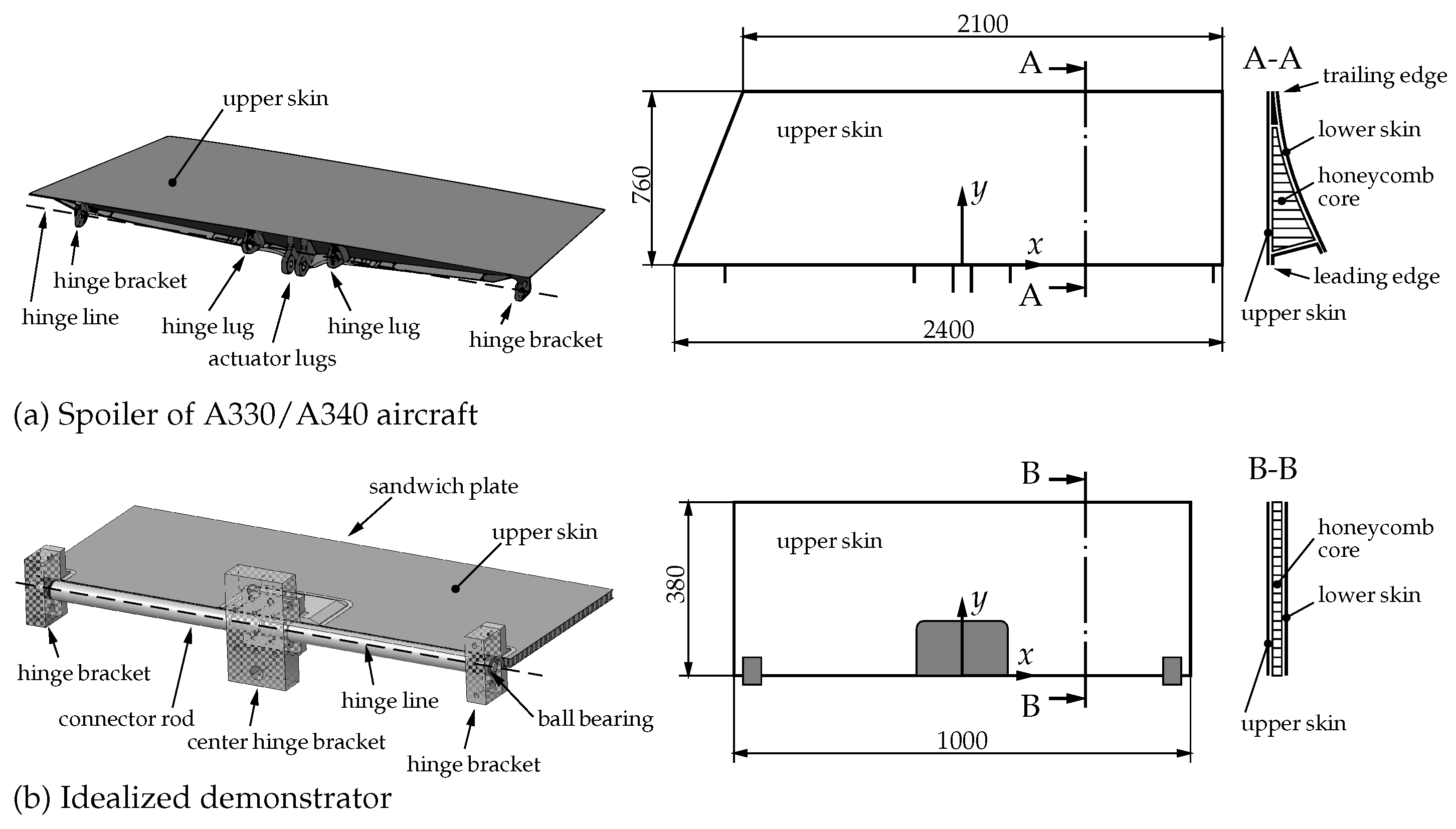
The demonstrator includes several simplifications compared to the real spoiler. Its overall size was scaled down by a factor of 1:2 and the original asymmetric shape was simplified to a rectangular shape. Additionally, the wedge-shape sandwich structured composite was approximated by a standard sandwich plate with a constant thickness. More specifically, it is a 15 mm thick sandwich plate with a Nomex honeycomb core and glass fiber-reinforced plastic (GFRP) layers on its top and bottom surface. Each GFRP layer is 0.5 mm thick and consists of four prepreg fabric plies with fiber orientations [0, 45, −45, 0]. Lastly, the hinge components of the real spoiler were simplified by less complex aluminum hinge brackets [21,23]. The overall dimensions of the demonstrator, as well as the outlined simplifications, are illustrated in Figure 1.

The spoiler demonstrator is designed to reproduce the spatial strain states, which the upper surface layer of the real spoiler experiences when it is deformed by the aerodynamic pressure caused by a 35° extension immediately after touchdown of the aircraft. This scenario is referred to as the design load case. In order to reproduce the deformation state of the real spoiler, the demonstrator is deformed by a whiffle tree. This mechanism enables a defined force distribution across multiple introduction points via mechanical linkages [23].

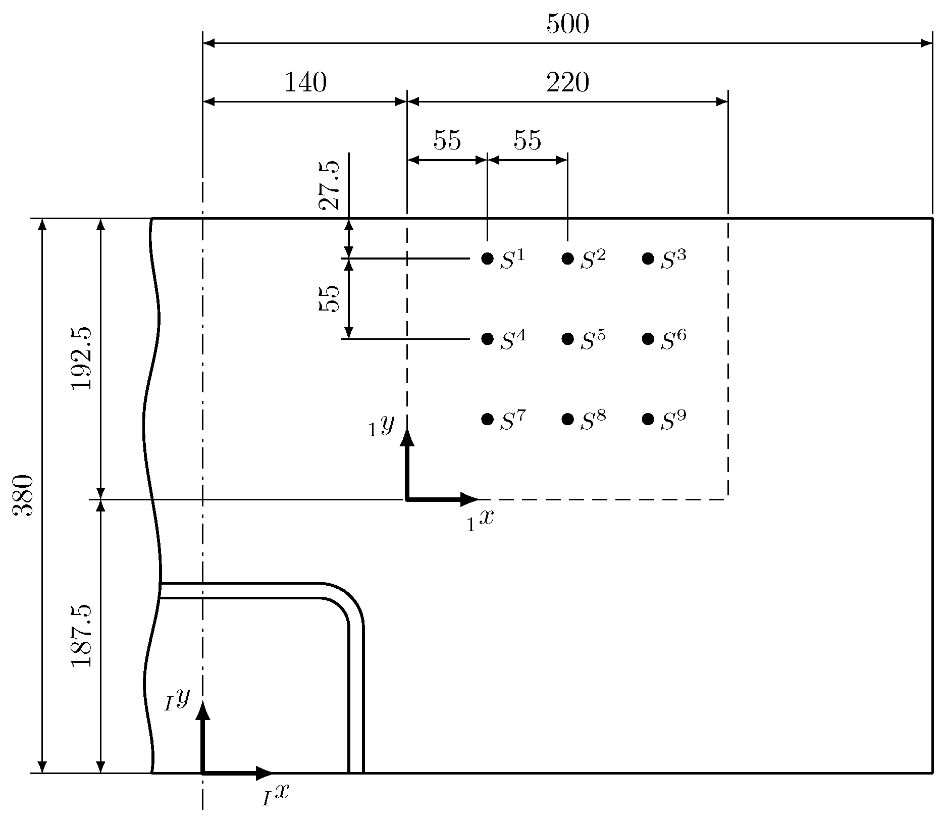
A grid of strain gauge rosettes HBM RY93-6/120 (HBM GmbH, Darmstadt, Germany) is applied to the surface of the demonstrator, close to its trailing edge, where all sensors are spaced 55 $\mathrm{m}$$\mathrm{m}$ apart. Each strain gauge rosette measures strain in 0°, 45° and 90° directions [20]. Figure 2 shows the relevant dimensions and location of the sensor grid on the spoiler demonstrator.

Parallel to the mechanical build of the demonstrator, Winklberger et al. [23] created a detailed numerical 3D model in the FE software Abaqus/Standard 2019 [24]. The symmetric forces (with respect to the $yz$-plane) introduced by the whiffle tree are represented in the FE model by nodal forces, the magnitude and location of which are controllable parameters. The sandwich core was modeled with continuum elements C3D8R (average mesh size: 10 mm × 10 mm × 7.5 mm). The GFRP layers on the top and bottom surface of the sandwich core were modeled using the composite layup feature provided by the property module in Abaqus. The surface layers are discretized by conventional shell elements S4R and an average mesh size of 10 mm × 10 mm.

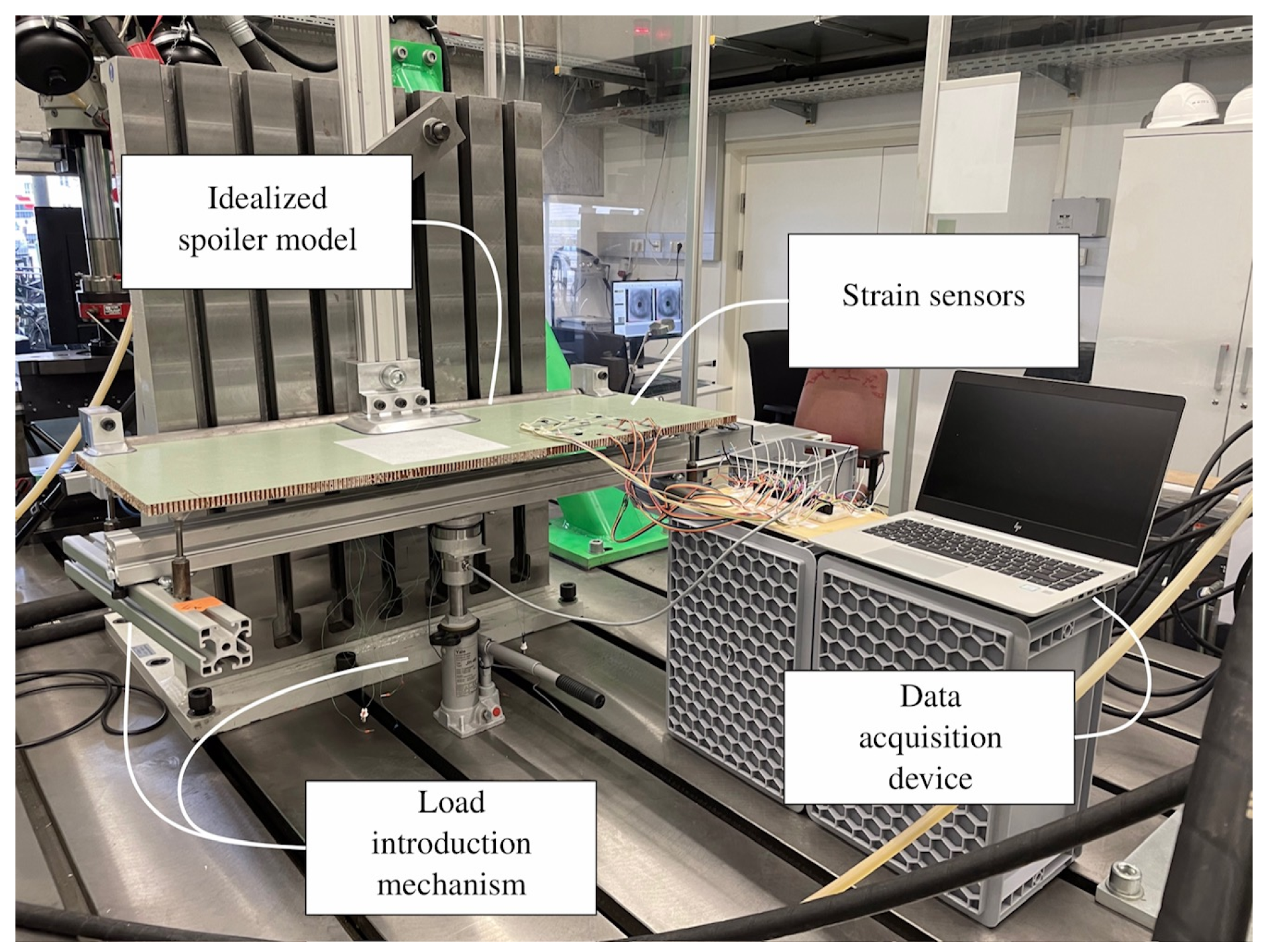
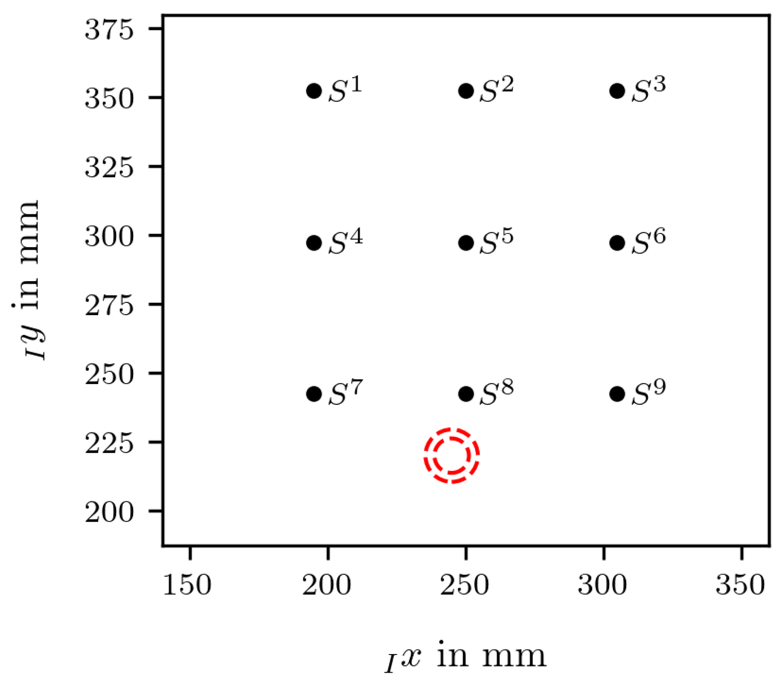
In the course of prior studies utilizing the demonstrator, two damages in the form of different sized holes were introduced. First, strain data due to five unique load cases was acquired from the pristine spoiler. In a following step, a 12.5 mm diameter hole was drilled just below sensor 8 and strain measurements were again conducted for the same load cases as used for the pristine case. Lastly, the same procedure was repeated after enlarging the existing hole to a diameter of 19 mm. This data represents the available experimental test data; thus, there are 15 samples with strains of three different health states (pristine and damaged by hole with diameters 12.5 mm and 19 mm) [20]. The corresponding experimental setup is depicted in Figure 3.

The location of the damages on the spoiler demonstrator, in relation to the sensor grid, are depicted in Figure 4. To easily denote specific sensors in the following, the notation $S_j^i$ has been introduced, where i is replaced with the position number and j with the measurement direction. The directions x, $\xi$ and y correspond to the sensor coil orientations 0°, 45° and 90°, respectively. If the directional index is not given, all directions are considered.

2.2. Synthetic Training Data

A prerequisite for the generation of synthetic training data is an existing FE model of the structure which is to be monitored. The FE model is utilized to simulate different load cases, from the results of which strain data is then extracted for its intended use as training data. In order to acquire strain data which covers a broad range of load cases, i.e., to achieve high variance training data, a large number of unique simulations is necessary.

In the presented work this computational effort is reduced by utilizing a framework for physics-driven feature generation of strain data for the training of ML-based SHM methods, developed by Bergmayr et al. [21]. It uses the FE model and the simulation results of a single, specific load case to generate a large amount of strain data representing new hypothetical, but physically probable, load cases. Therefore, these load cases do not require a simulation, but are instead derived from this objective load case.

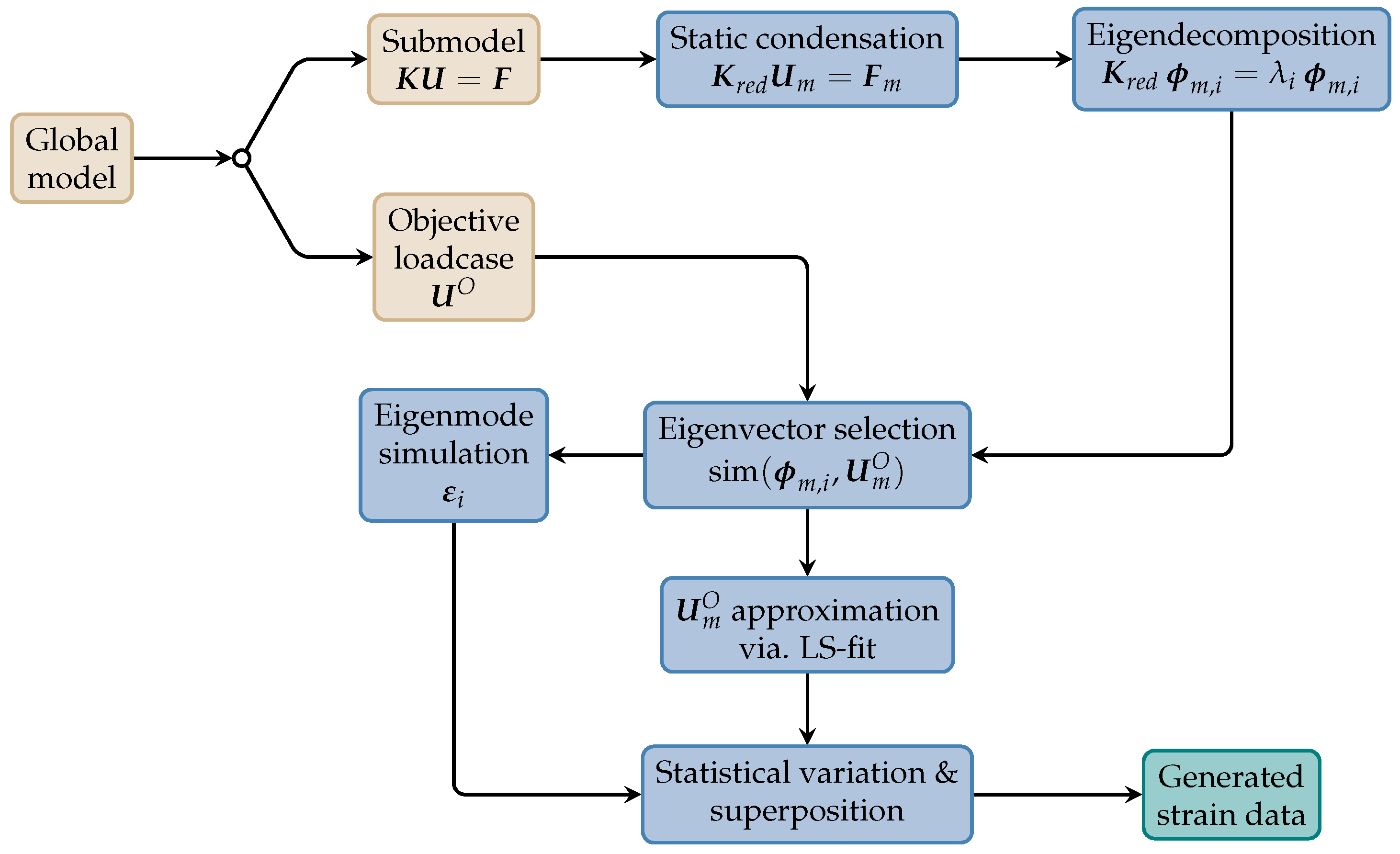
The framework, illustrated in Figure 5 as a process flow, is closely linked to the FE model of the structure. In its current state, it requires that the area of the sensor grid is modeled as a submodel using the sub-structuring technique [21,24]. The FE model of the complete structure represents the global model in this context. When the global model is simulated with an objective load case, the resulting displacements at the submodel edges become available. These then serve as boundary conditions for the simulation of only the submodel, but with refined geometry and mesh settings. The framework uses these objective load case displacements ${\mathit{U}}^O$ and the stiffness matrix $\mathit{K}$ of the submodel as inputs. The stiffness matrix is further reduced in size through a static condensation procedure. For this, it is assumed that no external forces are applied to the submodel, i.e., the relevant displacements result from the boundary conditions at the master nodes, introduced by the loaded global model [21]. The corresponding sub-matrices and sub-vectors are denoted by the subscript m. In a following step, the eigenvectors ${\mathit{\varphi }}_{m,i}$ of the resulting reduced stiffness matrix ${\mathit{K}}_{red}$ are calculated, where $i=1\dots N_m$ and $N_m$ is the size of the quadratic matrix ${\mathit{K}}_{red}$. Those eigenvectors which best approximate the objective load case displacements ${\mathit{U}}_m^O$ are selected for further processing steps. The set of best fitting eigenvectors is denoted as $E_B$. A linear combination of all eigenvectors with the corresponding optimal coefficients $x_i^O$, where $i\in E_B$, is able to closely replicate the objective load case displacements. The coefficients $x_i^O$ are determined for the selected eigenvectors through a least squares optimization with respect to the objective load case displacement:

$$\underset{\mathit{x}}{\min }∥{\mathit{U}}_m^O-\sum _{i\in E_B}{\mathit{\varphi }}_{m,i}{x}_i∥$$

(1)

By applying the elements of the individual eigenvectors as displacements at the submodel edges (instead of the objective load case displacements), strain data ${\epsilon }_i$ acquired using each eigenvector is obtained. The superposition of this eigenvector strain data, additionally scaled with the optimal coefficients, again results in approximately the same strain data as it would result from a simulation with the objective load case displacements at the submodel edges.

By statistically varying the optimal coefficients according to

$${\tilde{x}}_{i,l}^O\sim x_i^O\mathcal{U}(1-u,1+u),$$

(2)

strain data using an artificial but physically plausible load case—similar but not equal to the objective load case—can be derived:

$${\mathit{\epsilon }}_l^O=\sum _{i\in E_B}{\mathit{\epsilon }}_i{\tilde{x}}_{i,l}^O\mathrm{with}l=1,\dots ,N_g$$

(3)

The deviation parameter $u\in [0,1)$ controls the width of the uniform distribution $\mathcal{U}$, i.e., to which extent each parameter is varied. The number of newly generated samples is represented by $N_g$. This way, a large amount of new, physics-driven strain data due to arbitrary load cases is generated in a computationally inexpensive manner.

Figure 5. Simplified process flow of the framework. Brown boxes denote FE-specific process steps (FE domain). Blue boxes denote steps as part of the framework implementation [21].

Figure 5. Simplified process flow of the framework. Brown boxes denote FE-specific process steps (FE domain). Blue boxes denote steps as part of the framework implementation [21].

The original concept and implementation of the framework focused mainly on the generation of strain data derived from one specific objective load case. In the course of this work, the framework was further automated and extended, such that the generation of strain data derived from multiple different objective load cases is possible in a fast and efficient manner. Through this, more diverse training data can be generated, enhancing not only its quantity, but also its quality. An in-depth description of the framework can be found in the original publication by Bergmayr et al. [21].

2.3. Model Architecture and Training

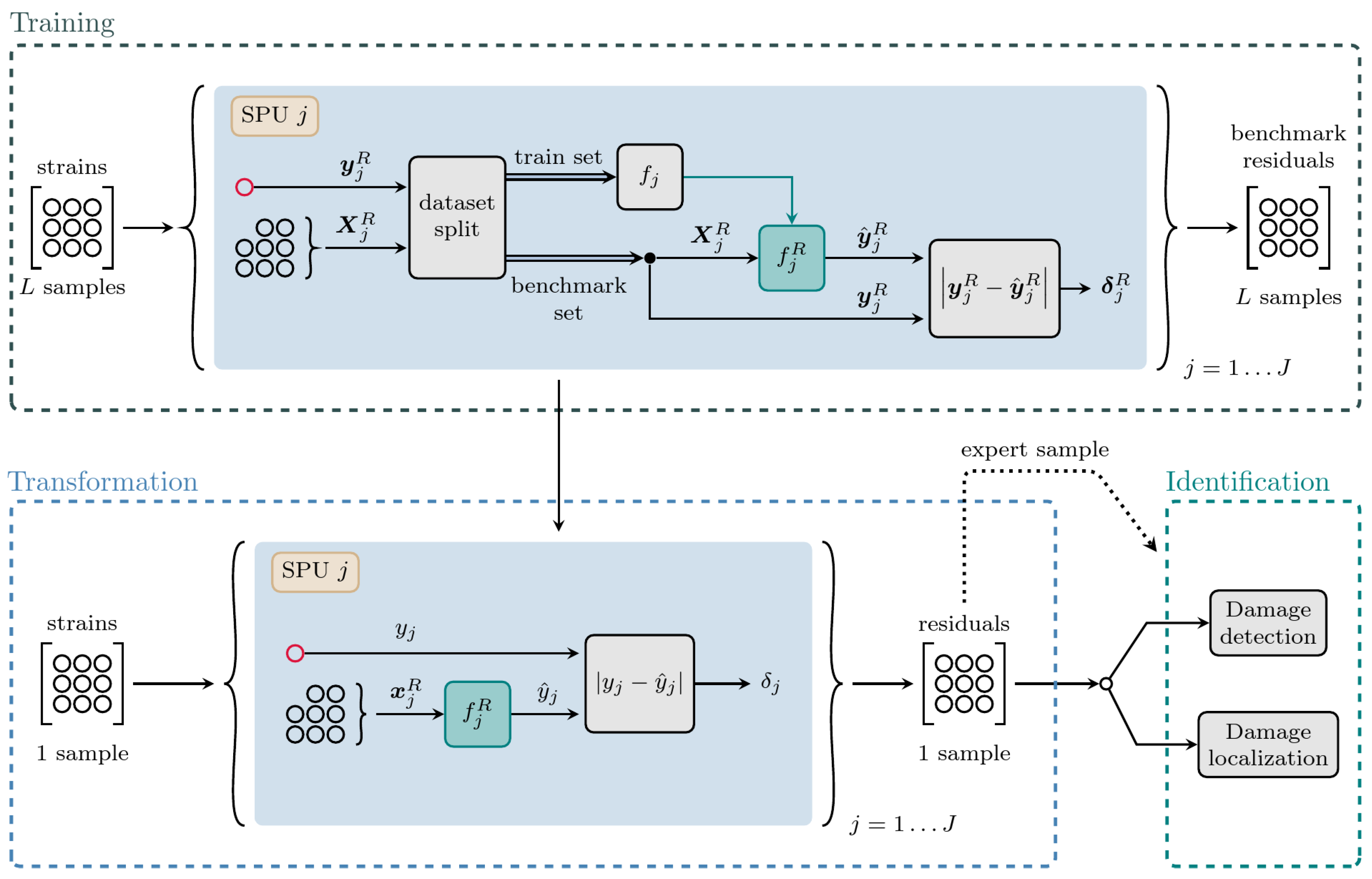
The proposed SHM application now utilizes the physics-driven, synthetic and pristine training data for the identification of damages in strain sensor data acquired from the real structure. The underlying concept is to learn the behavior of each strain value based on the behavior of all other strain values. In unseen data, each strain value is isolated and the remaining strain values are used as input to predict the value of the isolated element. The resulting prediction error is finally used as an anomaly score, characterizing the health state at the corresponding sensor location. The outlined task is broken down into three main process steps, namely training, strain data transformation and damage identification.

To learn the relationship between strain sensor values, the developed overall model consists of an ensemble of regression models, which is governed by the layout of the sensor grid providing the data. Each strain value measured by the sensor grid is considered as a feature j, where J is the total number features.

In the training stage, the synthetic training data is first separated into feature data ${\mathit{X}}_j^R\in {\mathbb{R}}^{L\times J-1}$ (strain values which are used for the prediction) and a target label ${\mathit{y}}_j^R\in {\mathbb{R}}^L$ (target strain which is to be predicted), where L denotes the number of samples and R denotes the reference configuration of the structure, i.e., the pristine state. This data is then further split into a training and a benchmark set. A regression model $f_j$ is subsequently fitted with the training data, resulting in the trained model $f_j^R$. With this, the benchmark set is passed to $f_j^R$, which provides predictions ${\widehat{\mathit{y}}}_j^R$. The residual ${\mathit{\delta }}_j^R\in {\mathbb{R}}^L$ is then calculated element-wise using the absolute error

$${\mathit{\delta }}_j^R=\left|{\mathit{y}}_j^R-{\widehat{\mathit{y}}}_j^R\right|.$$

(4)

This serves as a benchmark for the following damage identification. The residuals of all features together define the benchmark residual set ${\mathbf{\Delta }}^R\in {\mathbb{R}}^{L\times J}$.

Now, when passing unseen strain data of the real structure to the trained model, the prediction results of the fitted regression model $f_j^R$ are again evaluated against the corresponding true strain value. For this, the sample, which is to be classified, is once more separated into feature data ${\mathit{x}}_j\in {\mathbb{R}}^{J-1}$ and target label $y_j$. The feature data is then directly fed as input to $f_j^R$, which produces a prediction ${\widehat{y}}_j$. The residual ${\delta }_j$ is calculated as in (4) and the vector of all J residual values of one sample is subsequently denoted as $\mathit{\delta }\in {\mathbb{R}}^J$.

When the fitted regression models $f_j^R$ are provided with strain values from a pristine structure, they are able to reproduce each strain j. In contrast, when they receive strain values from a damaged structure, there will be a larger difference between true and predicted value, consequently indicating an anomaly.

The above describes the transformation stage, in which sensor grid strain data from the feature space is transformed into a residual space, where variations due to different load cases are compensated and differences due to anomalies, such as damages, are emphasized. The described process is the same for all J features and is therefore summarized in a generic Strain Prediction Unit (SPU). Hence, each feature is transformed by its own SPU. The architecture and corresponding process flow of a single unit is visualized in Figure 6.

Theoretically, any regression model can be chosen for $f_j$, e.g., an ANN as chosen by Grassia et al. [19] or linear regression, as used by Bergmayr et al. [20]. For this SHM application, a Histogram-based Gradient Boosting Regression Tree (GBRT), provided by the scikit-learn 1.4.1 [25] package, was implemented in Python 3.11. It is a fast and effective off-the-shelf model and is not sensitive to the scale of its input data, in contrast to ANNs and linear regression [26].

Since there is an individual SPU for each feature j, there is the possibility to define a separate set of parameters for each unit. Also, due to the setup of the sensor grid, the units at each sensor position have unique prerequisites regarding the information contained in their input data. To give an example, the prediction of strain values at sensor 5 is based on strain values provided by four close-by sensors. These values additionally describe the strain state around sensor 5. In contrast, the prediction of strain values of an edge sensor, e.g., sensor 1, relies on only two close-by sensors. In this context, an attempt has been made to compensate the unequal spatial prediction prerequisites by training each SPU with an individual parameter set. Initially, the parameters of each SPU were determined via a 5-fold cross-validated grid search over the training data, using the GridSearchCV method of scikit-learn 1.4.1. The parameter ranges for the grid search were chosen to promote high sensitivity to variations and support the detection of anomalies in the experimental data during the damage identification step. It was found that the SHM application is more robust when the same parameter set is used for all SPUs. Therefore, the most frequently selected parameter values from the individual grid searches were adopted uniformly for all SPUs. The non-default histogram-based GBRT hyperparameter values are listed in

Table 1. Non-default parameter values used for the scikit-learn implementation of the histogram-based gradient boosting regression tree, together with the values used in the parameter grid search.

Parameter	Grid Searched Values	Final Value
Loss function of boosting process	-	absolute error
Maximum number of trees	$\{200,300\}$	300
Maximum depth of each tree	$\{\mathrm{None},40,60\}$	40
Maximum number of leaves for each tree	$\{31,40\}$	40
Minimum number of samples per leaf	$\{30,50\}$	50
L2 regularization parameter	$\{0,0.5\}$	0.5

.

In a final step, the available transformation results are processed for damage detection and localization.

2.4. Damage Detection

The detection task, given the transformed strain data, is broken down to determine an appropriate threshold, which can reliably separate pristine samples from damaged ones. With the assumption that the transformed data shows high values at features spatially close to a damage and otherwise values close to zero, the following damage detection strategy is implemented: Given a matrix of transformed benchmark residual data ${\mathbf{\Delta }}^R$, the row-wise (i.e., feature-wise) median is calculated as

$$\mathrm{median}\left({\mathbf{\Delta }}^R\right)={\tilde{\mathbf{\Delta }}}^R,$$

(5)

where ${\tilde{\mathbf{\Delta }}}^R\in {\mathbb{R}}^L$. The median is advantageous here because it is robust against possible bad prediction results in the benchmark data, i.e., high residual values. These can occur due to the nature of the generated data, which covers a broad range of physics-based, yet still hypothetical, load cases. Some of these might operate in quite unique value ranges and are therefore more difficult to predict. The result of Equation (5) is further generalized by computing the arithmetic mean over all sample medians

$$\mathrm{mean}\left({\tilde{\mathbf{\Delta }}}^R\right)={\tilde{\mu }}^R,$$

(6)

where ${\tilde{\mu }}^R$ represents the lowest bound for a decision threshold t.

A major challenge in the given classification task is to account for the discrepancy between numerical model and the real structure. A straightforward approach to address this is to introduce a known, pristine expert sample in the form of a residual ${\mathit{\delta }}^E\in {\mathbb{R}}^J$ from the available experimental data. In an application scenario, such an expert sample could be easily acquired during the initial setup of the SHM application with the target structure. With this sample available, its arithmetic mean over all features is computed as

$$\mathrm{mean}\left({\mathit{\delta }}^E\right)={\mu }^E,$$

(7)

which yields a lower bound ${\mu }^E$ for the test data. Since the goal is to identify outliers, it is sensible to compute the mean, which is more sensitive in this regard.

A transformed sample of a pristine structure is expected to have a mean value that is close to ${\tilde{\mu }}^R$ or ${\mu }^E$. In the worst acceptable case, it might possibly have a value slightly higher than ${\mu }^E$. The inclusion of such a sample is controlled by a tolerance parameter $\gamma \in \left[0,1\right]$. The threshold t is then computed as

$$t=\max \left\{{\tilde{\mu }}^R,{\mu }^E\right\}·(1+\gamma ).$$

(8)

The edge-case, where the mean of an expert residual ${\mu }^E$ is smaller then that of the lowest bound of the benchmark data ${\tilde{\mu }}^R$, is covered by the maximum value function. The detection of damage in a given test sample $\mathit{\delta }\in {\mathbb{R}}^J$ ultimately comes down to the decision rule

$$\mathrm{mean}\left(\mathit{\delta }\right)>t.$$

(9)

If the condition (9) is fulfilled, the SHM application labels the test sample as damaged, or otherwise as pristine. The mean of the transformed test sample $\mathrm{mean}\left(\mathit{\delta }\right)$ can also be interpreted as a damage index.

2.5. Damage Localization

Due to the fact that the SHM approach requires that a sensor grid in some form is applied to the monitored structure, where a prediction unit is assigned to each sensor, it is also possible to locate damages. To demonstrate this, a straight-forward approach is proposed, where the residuals ${\delta }_j$ of a specific test sample $\mathit{\delta }$ are interpolated inside the sensor grid area. Specifically, the meshgrid function of the numpy 1.26.4 python module is used to construct an evenly spaced grid of coordinates over the submodel area. These coordinates are then passed, together with the coordinates of the sensors and the corresponding transformed data values, to the griddata function of the python module scipy 1.12.0. This function interpolates the transformed data values at the grid coordinates, using a cubic spline.

The edges of the submodel, used in the generation of synthetic training data, are used as borders for the interpolation. Here, a value of 0 is assigned, based on the assumption that there is no damage located well outside of the sensor grid.

An anomaly somewhere inside the sensor grid will result in an increased residual value ${\delta }_j$ at sensors close to the damage measuring feature j, where the magnitude is proportional to the distance between damage and sensor. The coordinates corresponding to the maximum interpolation value are then considered as a damage location prediction.

3. Results and Discussion

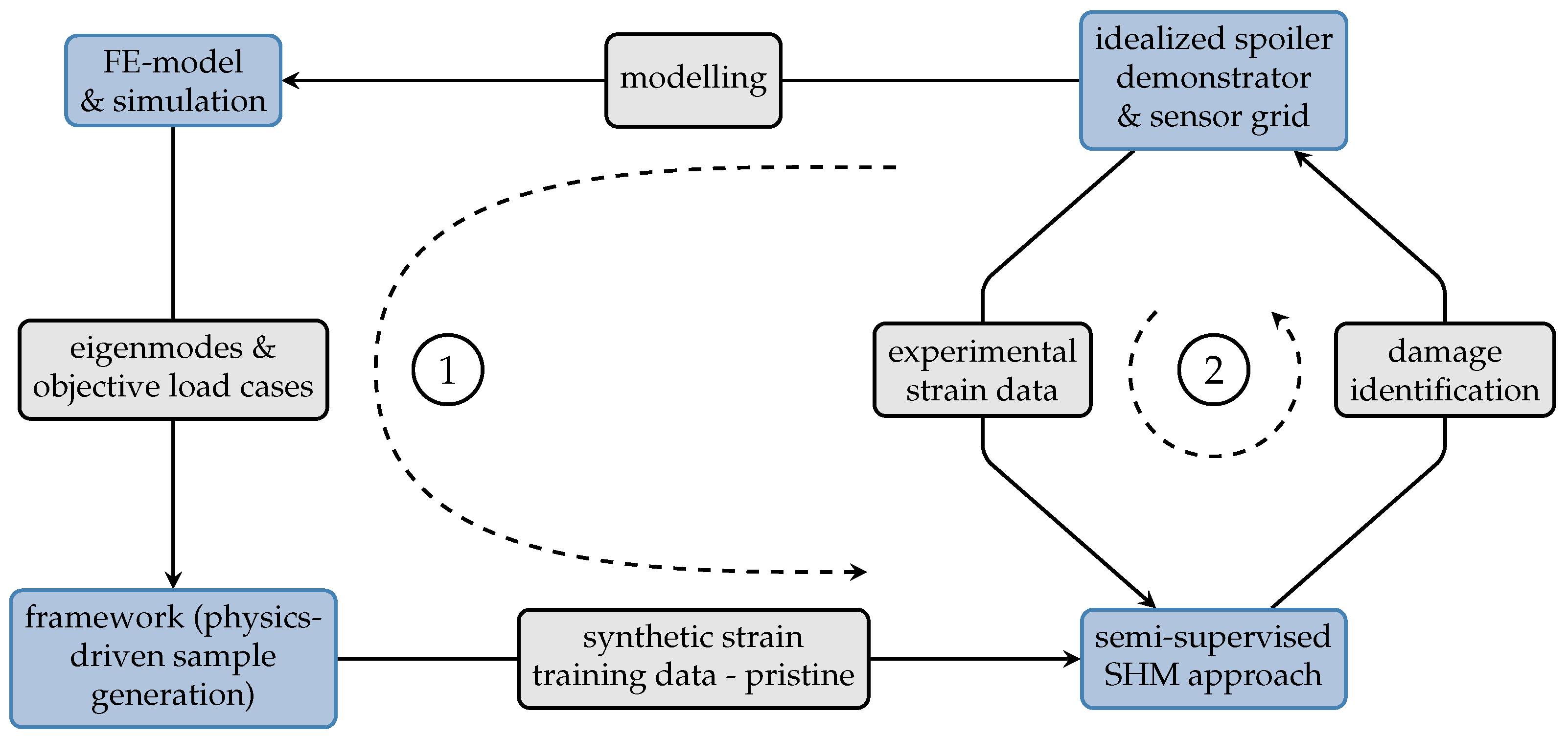
The SHM approach is applied to data of the spoiler demonstrator, introduced as a case example in Section 2.1. The 3 × 3 sensor grid (three-element strain gauge rosettes, HBM RY93-6/120) installed on its surface provides $J=27$ spatially discrete strain values (features) upon application of a specific, static load case. Parallel to the physical model, the corresponding numerical FE model is utilized by the aforementioned framework for the generation of a large amount of synthetic training data. An illustration of this workflow is provided in Figure 7.

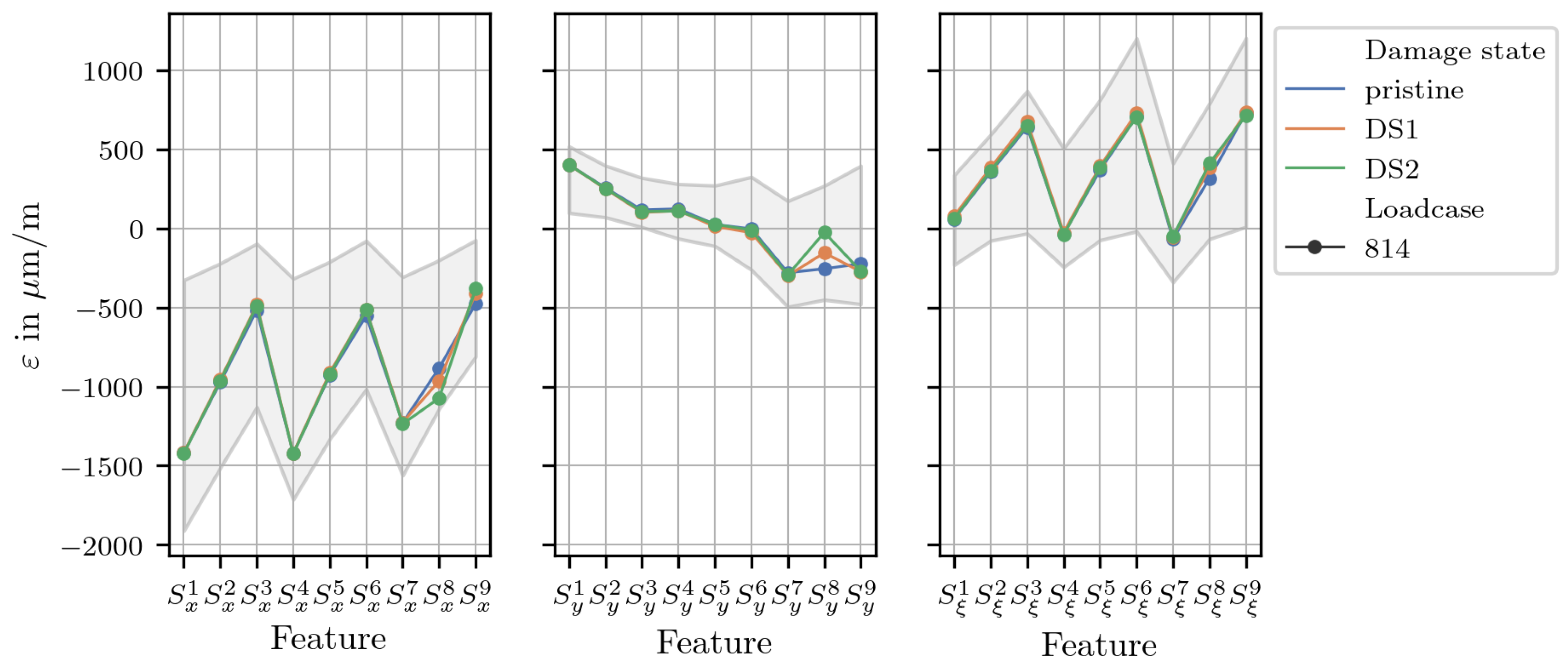
To provide more insight into the proposed SHM approach, the following section visualizes key aspects of the underlying data. Figure 8 compares the range of the synthetic training data, visualized by the grayed out area, with the experimental strain data measured on the spoiler demonstrator. The framework ultimately serves the goal of improving the robustness of a ML-based SHM approach by generating a large and diverse set of synthetic strain data that represents hypothetical, yet physically plausible, load case variations. This process functions as a form of physics-informed training data augmentation, aimed at improving the resilience to operational variability and unseen loading scenarios in the experimental data. The visualized data additionally shows the effect of a damage on the measured strains, as the individual data lines represent strains due to the same load case, but with different structural damages. The highest deviation from the pristine state can be observed at sensor 8, which is closest to the damage.

Following the training stage, unseen strain data from the spoiler demonstrator (experimental) is passed to the SHM model to be transformed into the residual space. The resulting residual values are visualized in Figure 9, together with a small number of transformed samples of the (numerical) benchmark set from the training stage.

As expected, the residual values of samples with different structural configurations is largest at sensors 7, 8 and 9.

Another view on the transformed data is achieved by a dimensionality reduction via Multidimensional Scaling (MDS). MDS maps high dimensional data to a lower-dimensional space while trying to preserve all pairwise distances of the data points [26,27]. Figure 10 shows the two-dimensional embedding of the transformed experimental data, together with a set of 40 randomly picked benchmark residuals.

In general, four visually distinct groups of points can be identified. The largest one is formed by the benchmark residuals. Closest to this is the group of pristine experimental residuals. The groups of damaged experimental residuals are located at a greater distance. Both are clearly distinguishable from each other, where the group containing residuals of the larger damage (diameter 19 mm) is located furthest away from the benchmark samples. This view on the data indicates a further challenge of the upcoming classification task, namely the generalization of the numerical training data to an extent such that real experimental data can be classified. In an ideal case, the pristine samples, regardless of their source, would not be distinguishable, i.e., as seen in the overlap in Figure 10. Here, without any labels, it is quite difficult to clearly ascertain if the pristine experimental samples are truly pristine or if they represent yet another damage state. This discrepancy can be reduced by an even better matching of a physical and numerical model or by the integration of specific system data before the classification stage. The latter strategy was chosen here in the form of including an expert sample in the decision threshold calculation.

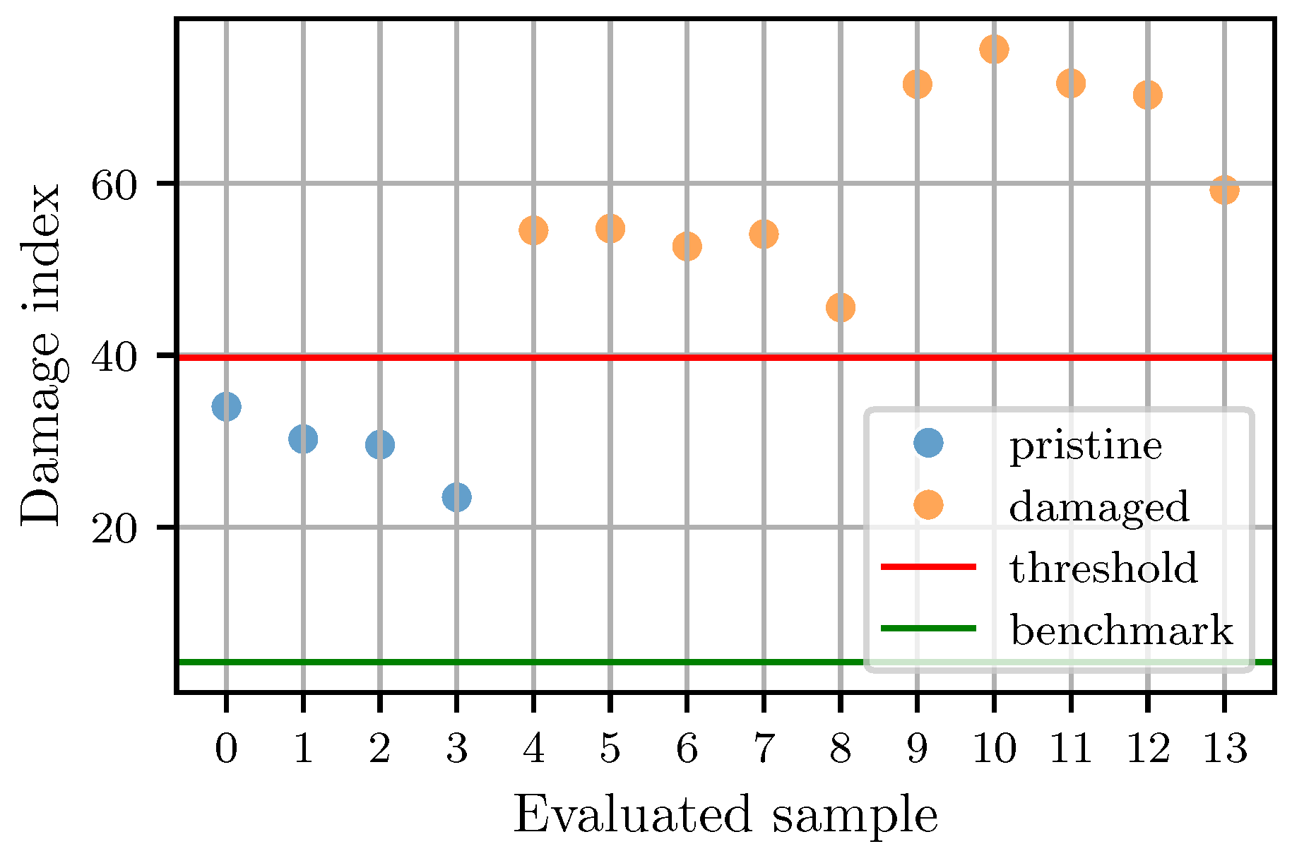
In the actual classification task, the transformed data is further utilized to calculate the corresponding damage index of each unseen sample as outlined in Section 2.4. When plotting the damage indices of all evaluated samples, depicted as colored points in Figure 11, there is again a clear distinction between the different structural states. The lowest bound of the benchmark set ${\tilde{\mu }}^R$ and the threshold t are additionally represented by horizontal lines. For the tolerance parameter, a value of $\gamma =0.3$ was used. The model classifies every sample with a damage index above the threshold as damaged and below it as pristine. This is consistent with the labeling of the data points; the model has a classification accuracy of 100%.

It should be noted that the computation of the threshold t is partly based on the empirical parameter $\gamma$, which controls the sensitivity of the damage detection. While the approach is intuitive, a more rigorous formulation remains a subject for future research. One possible direction could involve linking $\gamma$ to a statistical confidence level or to a similarity metric that quantifies how far the expert sample lies from the distribution of synthetic pristine data.

A further examination of the transformed data depicted in Figure 9 has shown that the model also allows specific conclusions to be drawn about the discrepancies between numerical and experimental model. This can be observed in the high residual values for all structural states at sensor 4, which suggest a systematic error. A closer inspection of the sensor grid on the spoiler demonstrator revealed that most sensors do not align perfectly with the positions used to extract strain data from the numerical model. Particularly, sensor 4 is slightly rotated counter-clockwise while all others are rotated clockwise. It can be shown that a rotational transformation of the measured strain data, which is easily achieved in a post-processing step, reduces the residual values at sensor 4.

Despite the misalignment between the numerical and experimental sensor grid and the almost unavoidable differences in the strain state due to modeling abstractions, the method is able to correctly classify damages. This confirms the method’s practical relevance and highlights its potential to detect real damage based solely on numerically generated pristine data.

In principle, the proposed SPU architecture is applicable to arbitrary structural shapes and sensor grid layouts, provided the sensor density suffices to measure effects of relevant discontinuities, and a pristine training set representing diverse loading scenarios is available. The strain field "fingerprint" of the structure is captured during training, while deviations at individual strain sensing points, which are not supported by the predictions of the ensemble of the remaining SPUs, indicate anomalies. This architecture is independent of the structure’s geometry, as well as the spatial layout of the sensor grid, though full validation remains for future work. Training with synthetic data additionally requires accurate knowledge and pairing of the sensor positions, as shown previously.

The experimental strain data is also used to demonstrate the localization capability of the SHM approach, resulting from the model architecture and a known sensor grid layout. Figure 12 shows the damage heat map due to the interpolation of residual values ${\delta }_j$. Unfortunately, on the spoiler demonstrator, the damage is placed outside of the sensor grid, making the experimental samples not ideal for the evaluation of the model’s localization performance, since the assumption of zero residuals at the sensor grid perimeter significantly influences the result there. Nonetheless, the actual location of the damage and its prediction match quite well.

4. Conclusions

A semi-supervised SHM approach has been presented, which is capable of detecting and localizing damages in spatially discrete strain data of a real structure. This is achieved by solely learning the pristine structure’s behavior under load from synthetic strain data, which is derived from simulations of a corresponding numerical model. The SHM approach is independent of environmental variables, like varying loading scenarios. There is no need to train the method with a specific damage characteristic, in contrast to conventional supervised ML approaches in SHM that require labeled damage data [13,14,15].

The localization of the damage is possible due to the sensor-wise architecture of the method and the known grid setup. This approach also illustrates one of the challenges of strain-based SHM methods quite well when it comes to monitoring larger structures. Damages or discontinuities in a structure only affect the strain field in their local vicinity. This implies a lower bound on the number of sensors and their density required on the structure [4]. The FOSs have shown considerable potential in this context due to their spatial resolution and their ability to be embedded in or applied to complex composite structures [1,3]. Compared to conventional strain gauges, they are well suited for denser sensor layouts and can be tailored more effectively to the geometry and loading characteristics of the monitored structure. This enables the optimization of sensor grid design to improve sensitivity and coverage [10,28]. Since a regular, evenly spaced sensor grid layout is not a mandatory requirement of the SHM approach presented in this work, applying FOS technology represents a promising direction for future research.

In the context of data-driven SHM, however, the ability to measure the strain field alone is not sufficient. For SHM Levels 2 and above, supervised learning approaches are typically required, which in turn depend on labeled damage data at the training stage. This data is typically rarely available [4,29]. As shown in this work, the utilization of synthetic training data mitigates this problem to some extent, but there is much more potential. Recent research focuses on approaches like federated learning [30,31,32] or population-based SHM [4,33]. The latter leverages transfer learning techniques, specifically domain adaption, to increase the available data by moving from a single structure to a population of structures. Through the functional abstraction of structures, the diagnosis of a data-poor target structure is enabled when there is a data-rich source structure similar enough to the initial one. Promising results have been reported in applications such as rotary machine monitoring, using transfer learning techniques like domain-adaption and fine-tuning [34]. These techniques present an interesting direction of further research, as they promise to improve the matching of physical and numerical models.