Towards a Digital Twin for Open-Frame Underwater Vehicles Using Evolutionary Algorithms

Abstract

Hydrodynamic coefficients determine the behavior of all simulated underwater vehicles. Therefore, it is essential to precisely define their values when aiming to replicate a real vehicle. Generally established procedures for obtaining them tend to have limitations, especially in transient responses. To address these issues, this paper proposes a comprehensive methodology for obtaining the hydrodynamic coefficients of an underwater vehicle. The main novelty is the combination of empirical measurements as a first step and evolutionary algorithms as a final step for optimizing the coefficients. The proposed methodology is described and applied to a commercially available remotely operated vehicle (ROV) BlueROV2, followed by analyzing the results in detail and including several tests that compare it to the real vehicle to validate its adequacy.

1. Introduction

Most of the tasks performed by autonomous underwater vehicles (AUVs) have focused on long-range exploration, mostly large torpedo-type AUVs designed for visually exploring and mapping large areas that require very long ranges [1,2]. Inspection and maintenance tasks for parts of the installation that are above water are similar to those performed in onshore installations and are reasonably standardized. Underwater inspections, however, are in a different state, as there are still no procedures or systems in place to carry out these operations in a systematic and cost-effective way. The applications of AUVs in these tasks, such as undersea structure inspection, are relatively new; although, some developments have been made in the oil and gas sector, especially following oil or gas lines [3] and some basic ideas proposed for windfarms [4].

To address these tasks, an approach based on the coordination of swarms of small and medium-sized underwater vehicles could be useful. This approach involves deploying a group of AUVs with autonomous navigation and behavior capabilities, equipped with the appropriate sensor set and sensing strategies, to carry out the analysis of the state of offshore structures. These tasks involve the AUVs not operating in open waters, but in more confined spaces, and have hardly been addressed except for some work on cave exploration [5,6]. Each AUV in the team needs to accurately determine its position with respect to the structure and the rest of the team.

A digital twin of the AUV that allows integrating the measurements made in real time with the simulations of the dynamic behavior of the assembly is proposed in this work. This makes it possible to determine the current situation of the vehicle while simulating and evaluating the future outcome of the decisions to be made by the system. Although parts of the developments in other sectors are applicable to AUVs, the complexity of the environment in which it is located, the high nonlinearity of the environmental responses, and the high degree of interactions make this a very incipient area in the field of AUVs [7], especially when operating closely or in contact with large structures.

Understanding system behavior before real-world deployment is crucial for modern robotics. Digital twins (DTs) are especially valuable in marine robotics [8] where they support risk assessment, strategy optimization, and emergency planning [9] without exposing the physical system to danger. However, building high-fidelity virtual models and ensuring rapid data updates remain key challenges.

DT technology is expanding into cyber physical operation systems, allowing real-time interaction between physical robots and virtual environments. This integration is enhanced by virtual reality visualization and advanced physics engines, which simulate dynamic interactions—such as track-ground contact—with high accuracy. These innovations are validated through experimental comparisons and are paving the way for more stable, efficient, and intuitive underwater operations [8,10].

While DTs are widely applied in manufacturing and other sectors, their use in underwater environments is still maturing due to the complexity of marine modeling [11]. Nevertheless, ongoing research and technological integration are rapidly advancing the capabilities and impact of digital twins in marine robotics [12]. All these factors make the digital twin of AUVs an open problem today that requires not only a base platform but also specific models that allow representing the physical phenomena that take place during the activity of AUVs [7,13].

2. Related Work

Developing simulation tools has been a constant effort with the intention of offering a tool for all underwater works, as can be seen in reviews such as [8]. To model dynamic behavior, various aspects such as vehicle dynamics, propulsion, coefficients defining the model, and added masses need to be considered. In a more traditional simulation, all these models stay static while the vehicle evolves and changes; however, when working with a digital twin, both the vehicle and twin need to evolve together. This introduces a limitation into the evolution of the models as the evolution of the model also needs to be considered.

Regarding the dynamic model, it has been approached from multiple perspectives, covering a wide range of phenomena that can affect the dynamic behavior of underwater vehicles. Various strategies have been employed to validate the model, including numerical simulations, towing tank experiments, and wind tunnel tests. Early works, such as the dynamic behavior modeling of VideoRay Pro III, assume decoupled movements in the three axes [14]. In [15], low-cost sensors are used in real experiments to validate a simplified dynamic model, applied for AUV control in heading, pitch, and depth. Other cases, like [16], use finite element-based numerical examples to validate the dynamic modeling of umbilical cable effects on AUVs.

Dynamic models are also inferred from simulations using computational fluid dynamics (CFD) based on the meshing of the AUV’s three-dimensional (3D) model [17]. Additionally, some studies focus on simulating the dynamic behavior of simple solids, as in [18], where models are tested using finite volume methods and validated in a wind tunnel, analyzing the effects of different edge shapes in detail, with results extrapolated to a real ROV.

In [19], a numerical model for a BlueROV2 is proposed, using the open source CFD software OpenFOAM to cover the four main freedom axes, and numerically simulated by a Reynolds-averaged Navier–Stokes (RANS) solver. The model is contrasted with hydrodynamic force and moment data measured in real trials, subjecting the ROV to various perturbations caused by different current and flow conditions.

Concerning the effects of vehicle propulsion on the dynamic model, different approaches have been considered, often motivated by vehicle control. In [20], the through-body thruster model of a torpedo-type C-SCOUT AUV is generated and numerically simulated, including forces due to hydrodynamic effects on control surfaces. Propeller shaft velocity and ambient flow velocity are used in [21] to estimate axial flow velocity, with the propulsion map divided into zones for analysis of the incoming angle of ambient flow through numerical simulation.

Some works address the propulsion model of underwater gliders propelled by buoyancy modulation. For instance, ref. [22] uses computational and semi-empirical methods to analyze the behavior of three different vehicles, ref. [23] examines thruster interactions, and ref. [24] investigates the influences of external currents on the propulsion model, conducting experiments with a BlueROV2 restrained by eight cables in different orientations relative to the incoming flow, and under different propeller operating conditions. With the development of open source simulators like Gazebo, many researchers started developing plugins and extensions to improve the accuracy of the underwater environment simulation such as the UUV Simulator [11], where the added mass, buoyancy, and other hydrodynamics are modeled using the Fossen equations [25].

As for the parameters affecting each model, various works focus on different aspects, and ref. [22] studies hydrodynamic parameters for the equations governing motion, while ref. [26] estimates hydrodynamic coefficients of a ROV using free decay pendulum motion. Real data are obtained in tests with a planar motion mechanism (PMM) for experimental evaluation of hydrodynamic coefficients in [23,27]. Furthermore, ref. [28] experimentally identifies hydrodynamic parameters for the LAURS open-frame AUV in one and three degrees of freedom, and ref. [29] uses experimental inertial measurement unit (IMU) values from an underwater vehicle to compare with results obtained through the genetic algorithm-based identification of hydrodynamic coefficients. Both refs. [30,31] evaluate hydrodynamic coefficients of an AUV, validating them through CFD simulations and experimental tests using a PMM. Furthermore, ref. [32] conducts towing tank and free-floating experiments to determine hydrodynamic coefficients of a ROV in 2 degrees of freedom.

The study of damping and added mass parameters usually accompanies the dynamic vehicle model. For instance, ref. [33] uses COMSOL Multiphysics to estimate added masses and damping parameters in the 6 degrees of freedom. However, comprehensive studies simultaneously addressing dynamic modeling, propulsion modeling, coefficients, and added masses are common, as seen in [26,34,35]. A comprehensive review is presented in [36].

In this paper, several important steps toward the development of a complete digital twin for an AUV are described. Specifically, Section 3 presents a comprehensive methodology for keeping the digital model up to date by combining information from traditional tests and measurements with the support of evolutionary algorithms to characterize the dynamic behavior of an AUV. An application of this methodology, using a BlueROV2 and a genetic algorithm, is presented in Section 4. The model is then validated through real-world tests, and the differences between model predictions and experimental results are analyzed and discussed in Section 5. Finally, Section 6 presents the conclusions drawn from the work.

3. Methodology Description

Over time, the underwater vehicles and their equipment are updated due to mission requirements, to improve their performance, or by obsolescence. The changes could affect the software, the equipment, and even the vehicle itself, and including more precise sensors, more capable actuators, or modifying other physical aspects can be quite common. All those changes have an impact on the real vehicle, changing its behavior. To avoid the divergence in results over time between the simulation and the reality, the digital twin needs to evolve in parallel with the real vehicle. This evolution requires the incorporation of some changes into the digital twin. This can be translated into the need to perform specific tests and measurements over the real vehicle to adequately evaluate the effects.

One of the key aspects that is affected in most cases is the vehicle’s hydrodynamic behavior, particularly in the case of open-frame vehicles, whose geometry is highly dependent on the onboard equipment. In order to adjust the hydrodynamic model and accurately represent the real behavior, we propose a methodology based on evolutionary algorithms, which is described in this section. Figure 1 shows an overall diagram of the proposed process that is going to be explained in detail in the next subsections.

3.1. Digital Twin Setup

The first step involves creating an accurate representation by integrating various simulators and models and finding a way to have them communicate with the real vehicle. These models capture different aspects of the vehicle, such as its physical structure, sensors, actuators, electronics, and the environment in which it operates. The main purpose is to ensure that all necessary interactions and behaviors for the tasks that we want to perform are adequately represented, providing a solid foundation for subsequent simulations and analyses. Communication is also a crucial factor, as the simulated and real vehicle need to exchange information during the process.

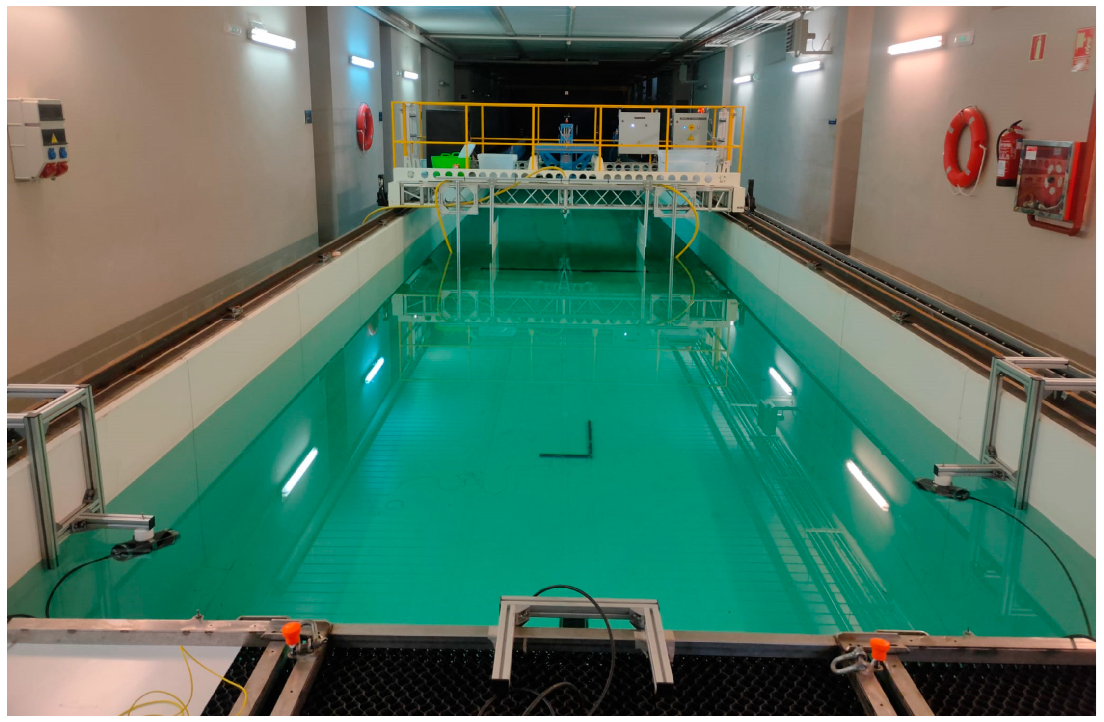
3.2. Real Tests and Measurements

Once the setup is ready, the next step is to conduct different tests and measurements with the real vehicle. These tests are crucial for obtaining precise and reliable data that will serve as a reference for all the different steps adjusting the digital twin. Some of the tests are going to be direct and simple measurements, while in other cases, it may be necessary to perform estimations based on the results of the towing tank tests, position or orientation values over time, etc. To ensure the accuracy of the simulation model, it is necessary to cover a wide range of operating conditions, and the tests should be designed in such a way that they allow the acquisition of all the information needed to accurately model the real vehicle’s behavior.

3.3. Hydrodynamic Model

Once the digital twin setup is established, the next crucial step is to estimate a hydrodynamic model, as a starting point for the optimization. There are many different methods to estimate the hydrodynamic coefficients; in some cases, they can be directly taken from similar vehicles in the literature [37]. In a more general approach, some methods are proposed in [38], including analytical methods, involving theoretical formulations and empirical correlations based on the vehicle geometry and operating conditions. Empirical methods involve conducting physical experiments, such as towing tank tests or free-decay experiments, to directly measure and observe the vehicle’s response in controlled conditions. Numerical methods, particularly CFD, simulate fluid flow around the vehicle under different conditions, offering detailed insights into complex interactions between the vehicle’s shape, propulsion systems, and surrounding fluid.

Both analytical and numerical methods can become quite complex, particularly when working with open-frame vehicles that present a complex geometry with holes and different shapes and a lot of equipment introducing disturbances (sensors, lights, cables, etc.). This leads to the empirical methods being the preferred in these applications as in [39], where the parameters of the dynamic model of the BlueROV2 have been determined and validated using both computer-aided design (CAD) software and physical experiments.

3.4. Optimization Algorithm

The previous estimation phase serves as a starting point, initializing the digital twin model for further refinement and validation through the proposed methodology. By combining the model with real data gathered from the vehicle, the hydrodynamic parameters of the model are optimized so the results of the simulations match the real data. This is a multi-objective problem, with a multitude of parameters to optimize, and a field where the use of a genetic algorithm (GA) has shown its flexibility and robustness.

GA is a stochastic, population-based optimization technique inspired by the process of natural selection and genetic evolution [40]. It operates by iteratively evolving a population of candidate solutions, with each solution represented as a set of parameter values. The optimization process aims to maximize a predefined fitness function, so that the simulated behavior closely matches empirical data from real-world trials.

3.5. Analysis of the Results

After the optimization process is finalized, the results are analyzed to detect some incoherencies or problems that could arise. The algorithm results are not filtered or directed in any way, only the upper and lower limits are considered for each parameter. The general idea with this step is to check for the feasibility of the results and to detect possible flaws. These flaws could be caused by some limitations on the model used, the fitness function considered, or the data-gathering process. However, they need to be adequately evaluated and addressed, if necessary, before the final validation tests.

3.6. Model Validation

The final step is to demonstrate the improvements achieved by the optimization process and the final state reached by the digital twin. This process involves conducting some tests with the real and simulated vehicles and a comparison of the results. This validation phase not only confirms the improvements made through optimization but also provides insights into future improvements and refinements of the digital twin over time.

3.7. Digital Twin Operation

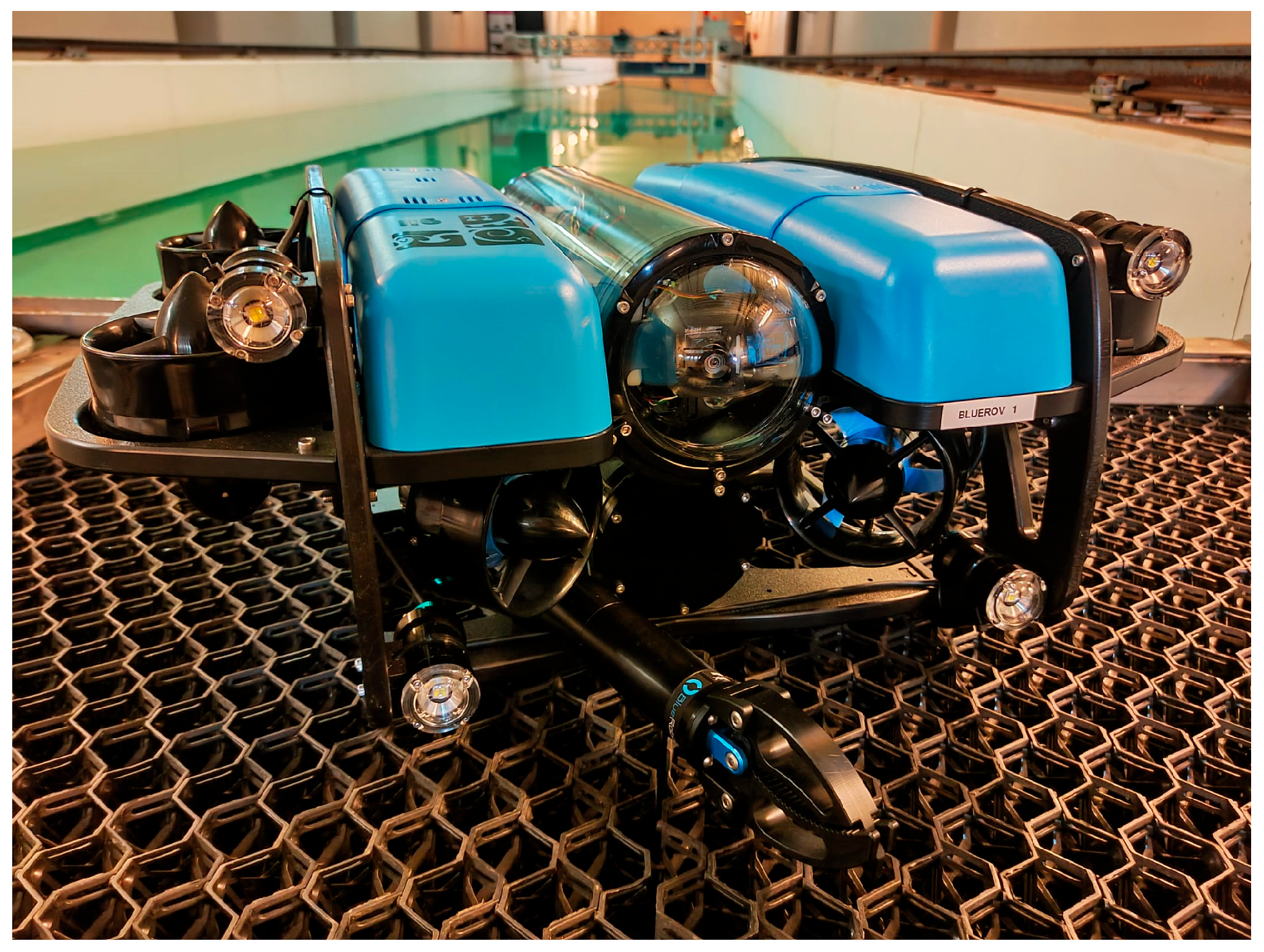
After the digital twin is adjusted and mimics the real vehicle’s behavior, it can be used as intended. During this stage, the digital twin allows the developers to test strategies using a realistic model of the real vehicle. This could be very useful for the development of novel coordination strategies, vehicle controllers, etc. This stage is only interrupted when there are significant differences between the real vehicle and the simulated twin. These changes are generally caused by modifications to the real vehicle required for a new task or project. When this happens, the process starts again, reusing everything from the previous iteration.

4. BlueROV2 Case

The vehicle selected for this work was a BlueROV2 from Blue Robotics Inc., an underwater open-frame ROV that has become very popular for its capabilities and affordability. More specifically, it was a BlueROV2 in its heavy configuration, with four horizontal propellers in a vectored position and the other four vertical propellers in each corner as shown in Figure 2.

The BlueROV2 was powered by an on-board Li-Ion battery that provided up to 6 h of operation, and it was controlled by a Pixhawk autopilot. It was equipped with an IMU and other sensors and actuators like a pressure transmitter, leak-detection sensors, a low-light HD camera, lights, and a gripper. Onboard, there was also a Raspberry Pi 3 that was used in this project for high-level autonomous behaviors and to communicate through the tether or umbilical cord to a topside computer that was used as a supervision tool as described in our previous publication [41].

4.1. Digital Twin Setup

To test the desired autonomous behaviors for the inspection and maintenance of offshore structures using underwater vehicles without risking them or their equipment, a complete simulation environment was set up. This environment relied on the Gazebo [42] simulator with the Unmanned Underwater Vehicle Simulator (UUV Simulator) package [11] to simulate physical effects, such as the propellers, water currents, interactions with other objects, etc., but also included the control logic of the autopilot.

This approach allowed the same code to be executed on both real and simulated vehicles and to even use them simultaneously and seamlessly to test coordination strategies. The mathematical modeling for the simulations was based on Fossen’s [43] equations. For this study, the Society of Naval Architects and Marine Engineers (SNAME) notation [44] was used, and a summary is shown in

Table 1. SNAME notation for marine vessels.

	Position and Angles	Linear and Angular Velocities	Forces and Moments
Movements	NED-frame	B-frame	B-frame
Surge	x	u	X
Sway	y	v	Y
Heave	z	w	Z
Roll	φ	p	K
Pitch	θ	q	M
Yaw	ψ	r	N

.

For a six-degree-of-freedom underwater vehicle, the matrix form of the equations of motion could then be expressed using the following:

$M_{RB}$ as the rigid-body matrix.

$\dot{\mathsf{\nu }}$ as the rate of change of the velocity $\mathsf{\nu }$ with respect to time.

$C_{RB}$ (ν) as the rigid-body Coriolis and centripetal matrix induced by $M_{RB}$ due to the rotation of the body frame about the north, east, down (NED) world frame.

$\mathsf{\nu }$ as the vehicle velocity vector.

$M_A$ as the added mass matrix.

$\dot{v_w}$ as the rate of change of the velocity $v_w$ with respect to time.

${ C}_A$ ($v_w$) as the added mass Coriolis and centripetal matrix induced by $M_A$ due to the rotation of the body frame about the NED world frame.

$v_w$ as the relative velocity vector.

$\mathrm{D}\left(v_w\right)$ as the damping matrix.

$\mathrm{g}\left(\mathsf{\eta }\right)$ as the restoring forces vector.

τ as a vector with all the external forces and moments actuating in the vehicle.

$$M_{RB}\dot{\mathsf{\nu }}+C_{RB}\left(\mathsf{\nu }\right)\mathsf{\nu }+M_A\dot{v_w}+C_A\left(v_w\right)v_w+\mathrm{D}\left(v_w\right)v_w+\mathrm{g}\left(\mathsf{\eta }\right)=\tau$$

(1)

The relative velocity vector $v_w$ can be calculated using the vehicle velocity $v$ and the current velocities in the fluid around the vehicle $v_c$ and thus be expressed as:

$$v_w=\mathsf{\nu }-v_c$$

(2)

A series of common assumptions when modeling underwater vehicles [45] could then be applied to simplify the equations and reduce the number of coefficients to be estimated:

• Assumption 1. The vehicle is assumed to be rigid, and 6 degrees of freedom (DOF) are considered.
• Assumption 2. The ROV is assumed symmetric around the front–back, port–starboard, and the top–bottom axes.
• Assumption 3. The body axes coincide with the main axes of inertia.
• Assumption 4. The origin of the b-frame is located at the center of mass of the vehicle.
• Assumption 5. The ocean current is modeled as a constant irrotational flow in the n-frame. Waves are neglected.
• Assumption 6. The movements for each DOF are assumed to be decoupled as they are performed at low speeds (less than 1 m/s).

The matrix expressions are detailed and explained in [43], but the most important ones are also included in this text to ease the lecture and interpretation. For symmetrical underwater vehicles during low-speed movements and with the gravity center on a vertical line from the coordinate origin (CO), the rigid body matrix $M_{RB}$ and the added mass matrix $M_A$ could be expressed using the following:

• $m$ as the mass of the vehicle in kg.
• $z_g$ as the vertical distance of the gravity center from the CO.
• $I_{XX}, I_{YY}$, and $I_{ZZ}$ as the moments of inertia for each axis.
• $X_{\dot{u}}, Y_{\dot{v}}, Z_{\dot{w}}, K_{\dot{p}}, M_{\dot{q}}, N_{\dot{r}}$ as the added mass coefficients for each degree of freedom (DOF).

$$M_{RB}=\left\{\begin{array}{cccccc}m& 0& 0& 0& m{z}_g& 0\\ 0& m& 0& -m{z}_g& 0& 0\\ 0& 0& m& 0& 0& 0\\ 0& -m{z}_g& 0& I_{XX}& 0& 0\\ m{z}_g& 0& 0& 0& I_{YY}& 0\\ 0& 0& 0& 0& 0& I_{ZZ}\end{array}\right\}$$

(3)

$$M_A=-diag\left\{X_{\dot{u}},Y_{\dot{v}}, Z_{\dot{w}},K_{\dot{p}},M_{\dot{q}},N_{\dot{r}}\right\}$$

(4)

The Coriolis matrixes can be expressed as:

$$C_{RB}\left(\mathsf{\nu }\right)=\left\{\begin{array}{cccccc}0& 0& 0& 0& mw& -mv\\ 0& 0& 0& -mw& 0& mu\\ 0& 0& 0& mv& -mu& 0\\ 0& mw& -mv& 0& I_{z}r& {-I}_{y}q\\ -mw& 0& mu& {-I}_{z}r& 0& I_{x}p\\ mv& -mu& 0& I_{y}q& {-I}_{x}p& 0\end{array}\right\}$$

(5)

$$C_A\left(v_w\right)=\left\{\begin{array}{cccccc}0& 0& 0& 0& {-Z}_{\dot{w}}w& Y_{\dot{v}}v\\ 0& 0& 0& Z_{\dot{w}}w& 0& {-X}_{\dot{u}}u\\ 0& 0& 0& {-Y}_{\dot{v}}v& X_{\dot{u}}u& 0\\ 0& {-Z}_{\dot{w}}w& Y_{\dot{v}}v& 0& {-N}_{\dot{r}}r& M_{\dot{q}}q\\ Z_{\dot{w}}w& 0& {-X}_{\dot{u}}u& N_{\dot{r}}r& 0& {-K}_{\dot{p}}p\\ -Y_{\dot{v}}v& X_{\dot{u}}u& 0& {-M}_{\dot{q}}q& K_{\dot{p}}p& 0\end{array}\right\}$$

(6)

The damping matrix is the combined expression of a lot of phenomena related to the interaction between the vehicle and the surrounding fluid, mostly dependent on the movement speed. It can be expressed as a second-degree polynomial of the movement speed for each axis, which implies two sets of parameters: one of them linearly coupled with the speed and one with the square of the speed.

$$\mathrm{D}\left(v_w\right)=D_L+D_Q\times \left|v_w\right|$$

(7)

$$D_L=diag\left\{X_u,Y_v, Z_w,K_p,M_q,N_r\right\}$$

(8)

$$D_Q=diag\left\{X_{u\left|u\right|},Y_{v\left|v\right|}, Z_{w\left|w\right|},K_{p\left|p\right|},M_{q\left|q\right|},N_{r\left|r\right|}\right\}$$

(9)

The restoring forces vector $\mathrm{g}\left(\mathsf{\eta }\right)$ depends on $\mathsf{\eta }$, the vector with the position and orientation of the CO relative to the navigation frame. For submersibles where the CO and center of gravity (CG) are in the same vertical line, they can be expressed using $W$ and $B$ as the weight and buoyancy of the vehicle, respectively, and $z_b$ as the vertical distance of the buoyancy center from the CO as:

$$g(\eta )=\left\{\begin{array}{c}\left(W-B\right)\sin \theta \\ -\left(W-B\right)\cos \theta \sin \phi \\ -\left(W-B\right)\cos \theta \cos \phi \\ -z_b B\cos \theta \sin \phi \\ -z_b B\sin \theta \\ 0\end{array}\right\}$$

(10)

Regarding the τ, the external forces and moments are primarily generated by the vehicle’s thrusters and can be estimated from their position, orientation, and thrust. These values have been included in the model, and the thrust generated by each propeller is calculated in real time using the thruster curve.

$$\mathsf{\tau }=\left\{\begin{array}{c}X\\ Y\\ Z\\ K\\ M\\ N\end{array}\right\}$$

(11)

4.2. Real Tests

A series of real tests and measurements were performed to gather all the information required to model the vehicle and evaluate it in different conditions. The main characteristics and equipment used for the tests are described in each one of the subsections that follow.

4.2.1. Propeller Modeling

As the only part introducing energy over the system, the thrusters need to be measured and adequately characterized. There are individual characterizations of the BlueROV2 thrusters available [46] that could be used to generate an estimated curve for the vehicle based on the number of thrusters and their orientation. However, the propeller flow when mounted on the vehicle is partially interrupted by its structure, cables, etc.

To adequately measure the real thrust, a series of tests were performed using an AXI 9195 DELTA IP68 triaxle load cell to measure the empirical curve of the thrusters mounted on the vehicle. The tests consisted of thrust and torque measurements with the thrusters of each axis actuated for a few seconds with different turning speeds. The thruster rotation speed was controlled using an electronic speed controller (ESC) with a pulse width modulation (PWM) input signal.

Figure 3 shows the measured and estimated thrust for the x axis ($X$) at different PWM values of the input signal (I). The first curve was obtained directly from the measurements, while the estimated one was obtained from the individual curves and the geometry configuration. In this specific case, assuming the same response for the four horizontal thrusters and $T$ as the individual thrust of each one, obtained from [46], we could express the estimated $X$ as:

$$X=4 T\cos {\displaystyle \frac{\pi }{4}}$$

(12)

There are noticeable differences between the two curves, especially in the region with high PWM signals. The same phenomenon appears on the y axis thrust, with similar intensity. On the z axis, whose thruster flow is unimpeded, the estimated and the empirical curves are almost identical.

4.2.2. Position and Orientation Tests

For the rotational movements (roll, pitch, and yaw), the tests consisted of movements in each axis at different thruster speeds. The motion was measured using the onboard IMU. For the linear motion tests (surge, sway, and heave), the ROV lacked a precise positioning system, so an underwater motion capture system from Qualisys was used. The system, shown in Figure 4, comprised a set of three Miqus underwater cameras that could detect and capture the motion of a body within a control volume up to 32 m³. After the control volume was calibrated, five markers were placed asymmetrically on the vehicle frame, and a virtual representation of the rigid body was defined. Finally, the tests were performed by moving the vehicle in each axis at different speeds, and the positions were captured over time.

4.3. Hydrodynamic Model

According to the measurements performed over the vehicle and some values from the literature, an initial hydrodynamic model was obtained. The results of all the estimations are shown in

Table 2. Initial estimations for hydrodynamic coefficients.

Parameters	Value	Units
$m$	13.17	kg
$B$	132.537	N
$CG$$(x_g$$, y_g$$, z_g$)	(0.0, 0.0, 0.0)	m
$CB(x_b,y_b,z_b)$	(0.0, 0.0, −0.024)	m
$I_{XX}$	0.344	Kg·m2
$I_{YY}$	0.316	Kg·m2
$I_{ZZ}$	0.389	Kg·m2
$X_{\dot{u}}$	13.272	Kg
$Y_{\dot{v}}$	13.123	Kg
$Z_{\dot{w}}$	14.508	Kg
$K_{\dot{p}}$	0.207	Kg·m2
$M_{\dot{q}}$	0.211	Kg·m2
$N_{\dot{r}}$	0.109	Kg·m2
$X_u$	−0.161	Kg/s
$Y_v$	−0.17	Kg/s
$Z_w$	−0.254	Kg/s
$K_p$	−0.349	Kg·m2/s
$M_q$	−0.221	Kg·m2/s
$N_r$	−0.141	Kg·m2/s
$X_{u\left|u\right|}$	−33.346	Kg/m
$Y_{v\left|v\right|}$	−45.731	Kg/m
$Z_{w\left|w\right|}$	−72.668	Kg/m
$K_{p\left|p\right|}$	−0.356	Kg·m2
$M_{q\left|q\right|}$	−0.461	Kg·m2
$N_{r\left|r\right|}$	−0.471	Kg·m2

. A precision scale was used to measure the mass and buoyancy of the vehicle, while the CG was determined by balancing the vehicle in each axis and measuring the distance from the outside structure. To obtain an estimation of the vertical distance between the center of buoyancy (CB) and the CG, a series of weights were added in one side of the vehicle, generating a roll moment that was equilibrated by the moment caused by the CB. The resultant roll angles were measured using the integrated IMU of the vehicle.

Regarding the moments of inertia, they were estimated using CAD commercial software SOLIDWORKS 2023, and a model of the vehicle, in which the weights of the main components (battery, electronics, and payload) had been added into their actual position. For added mass and damping coefficients, estimations were made based on the vehicle geometry and similar vehicles from the literature.

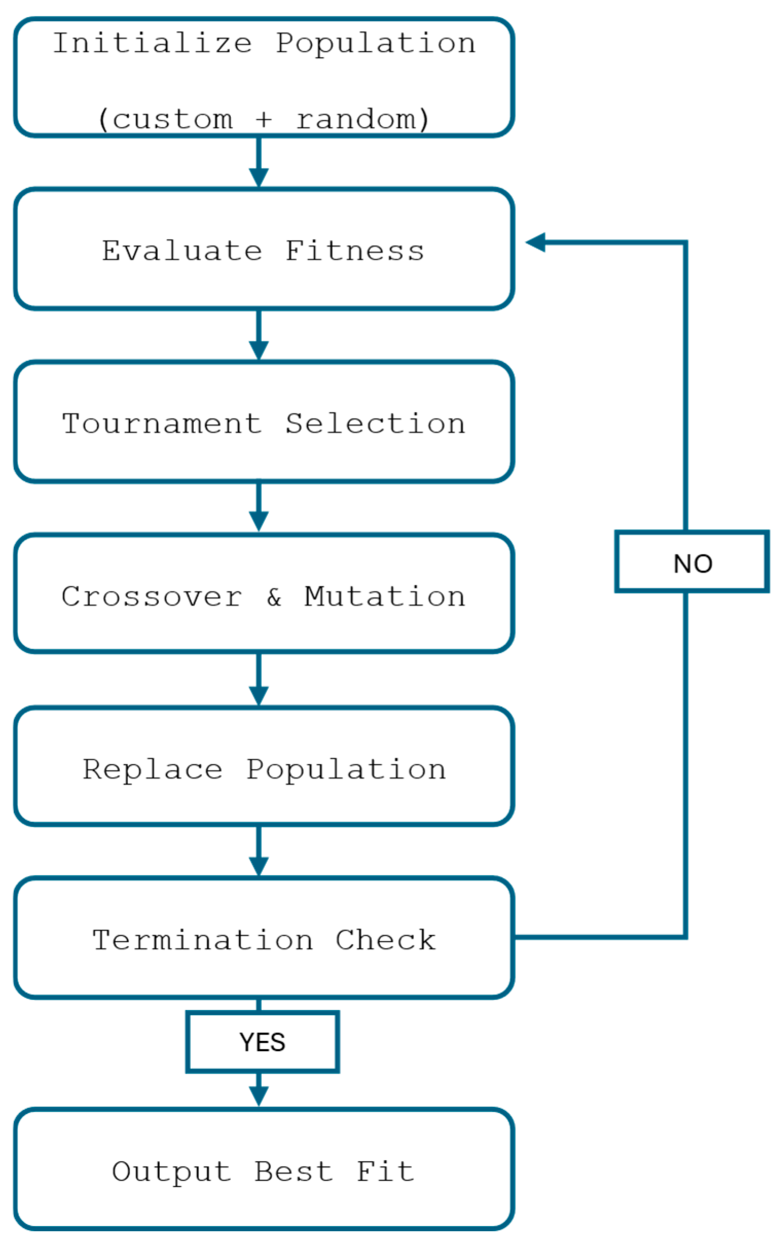
4.4. Genetic Algorithm

In this subsection, we provide a detailed description of the GA employed for optimizing parameter values in our study. In our specific case, a genetic algorithm from the Python DEAP library (version 1.4.1) [47] was selected to optimize the values of the hydrodynamic model. The optimization process, represented in Figure 5, began with the initialization of a population of candidate solutions. Each individual in the population represented a candidate solution composed of a set of dynamic parameters (e.g., added mass, damping coefficients, and inertia), and the algorithm evolved the population over several generations to maximize a fitness function based on the similarity between the simulated and real trajectories.

Each DOF was optimized individually, and the selected parameters for the optimization were different for each type of movement. For the linear movements, only three parameters were selected: the added mass, the linear damping, and the quadratic damping coefficients. For the rotational movements, the inertia was also included as a parameter, as its accuracy may not be good enough for the final modeling.

Table 3. Selected parameters for optimization.

Type of Movement		Inertia	Added Mass	Linear Damping	Quadratic Damping
Linear Movements	Surge	-	${\mathrm{X}}_{\dot{\mathrm{u}}}$	Xu	Xu|u|
	Sway	-	${\mathrm{Y}}_{\dot{\mathrm{v}}}$	Yv	Yv|v|
	Heave	-	${\mathrm{Z}}_{\dot{\mathrm{w}}}$	Zw	Zw|w|
Rotational Movements	Roll	Ixx	${\mathrm{K}}_{\dot{\mathrm{p}}}$	Kp	Kp|p|
	Pitch	Iyy	${\mathrm{M}}_{\dot{\mathrm{q}}}$	Mq	Mq|q|
	Yaw	Izz	${\mathrm{N}}_{\dot{\mathrm{r}}}$	Nr	Nr|r|

summarizes the parameters that were selected for each type of movement.

The range for each parameter was carefully chosen from the initial values listed in Table 2, with some reasonable margin up and down, so the algorithm could find the optimal parameters without using very broad limits. This was made with two ideas in mind: the first one was reducing the optimization time, as it is related to the search space size; and the second one was to avoid configurations that could produce similar numerical results on the simulation but were unreal, like positive damping coefficients. The main idea was to optimize the parameters, adjusting them, without losing all the original information from the real tests.

i.

Initialization

The first generation was partially initialized using specific parameter values obtained from experimental data. The rest of the individuals were randomly initialized within defined parameter ranges.

ii.

Evaluation

After initialization, each individual (candidate solution) was evaluated using a custom fitness function, which calculated the sum of absolute differences between the simulated and real data across multiple tests and degrees of freedom (DOFs).

iii.

Selection

The selection process determined which solutions will proceed to the next generation based on their fitness values. In our study, we employed tournament selection to choose parents for the next generation. This strategy involved randomly selecting a subset of solutions (tournament size = 5) from the population, and the one with the highest fitness was chosen. This method helped maintain diversity while applying selection pressure.

As previously stated, the fitness function evaluated the performance of each candidate solution in the population. It quantified how well the solution matched the desired behavior or characteristics of the system being optimized. In our study, the fitness function was defined as the sum of absolute differences between the ground truth data and the simulated data for each parameter over time.

The problem to solve is a multi-objective one. Even when considering each DOF as decoupled, there are multiple thruster speeds for each one. Specifically in this work, eight different thruster speeds were selected for each DOF. To find an optimal solution, the partial fitness functions for all these tests were combined, adding them into the final fitness function. A series of weights were applied in this process to improve the low-speed movements, as they were more interesting during the inspections.

iv.

Crossover

In the crossover stage, pairs of parent solutions were selected from the population based on their fitness values. These parent solutions underwent a crossover operation, where portions of their parameter values were exchanged to produce offspring solutions. The crossover operation introduces diversity into the population by combining beneficial traits from different parent solutions. In our implementation, we used a two-point crossover strategy with a probability of 0.5 to generate offspring, where two random points were selected along the parameter vectors, and the segments between these points were swapped between parents.

v.

Mutation

Following the crossover, the offspring solutions underwent a mutation operation, which introduced small random changes to their parameter values. Mutation helps to explore new regions of parameter space and prevents premature convergence to suboptimal solutions. We applied a Gaussian mutation operator, where random Gaussian noise was added to each parameter value with a mutation probability of 0.25, introducing variability to avoid local optima. The magnitude of the mutation was controlled by the standard deviation parameter.

vi.

Replacement

The offspring replaced the previous population, and the optimization process continued for a predetermined number of generations or until a termination criterion was met. Common termination criteria include reaching a maximum number of generations, achieving a satisfactory level of fitness, or observing negligible improvement over successive generations. In our case, we established a maximum of 30 generations. Once the termination criterion was satisfied, the algorithm returned the fittest solution found during the optimization process.

Table 4. Summary of genetic algorithm settings.

Stage	Description	Parameter Values
Initialization	Custom initialization for the first generation; standard initialization for subsequent generations	Specific parameter values; random parameter values within predefined ranges Population size: 60
Fitness Function	Sum of absolute differences between ground truth and simulated data	-
Selection	Tournament selection strategy	Tournament size: 5
Crossover	Two-point crossover strategy	Cross rate: 0.5
Mutation	Gaussian mutation operator	Mutation rate: 0.25
Termination	Maximum number of generations	Generations: 30

summarizes all the relevant parameters and information related to the genetic algorithm.

It is important to highlight that the novelty in our implementation lay in the custom initialization of the first generation using experimentally informed parameters, which biased the search toward realistic solutions. Additionally, multiple DOFs were optimized independently, and the fitness function combined the outcomes of multiple tests with a weighted approach to emphasize low-speed movement accuracy, an aspect critical in underwater inspection scenarios.

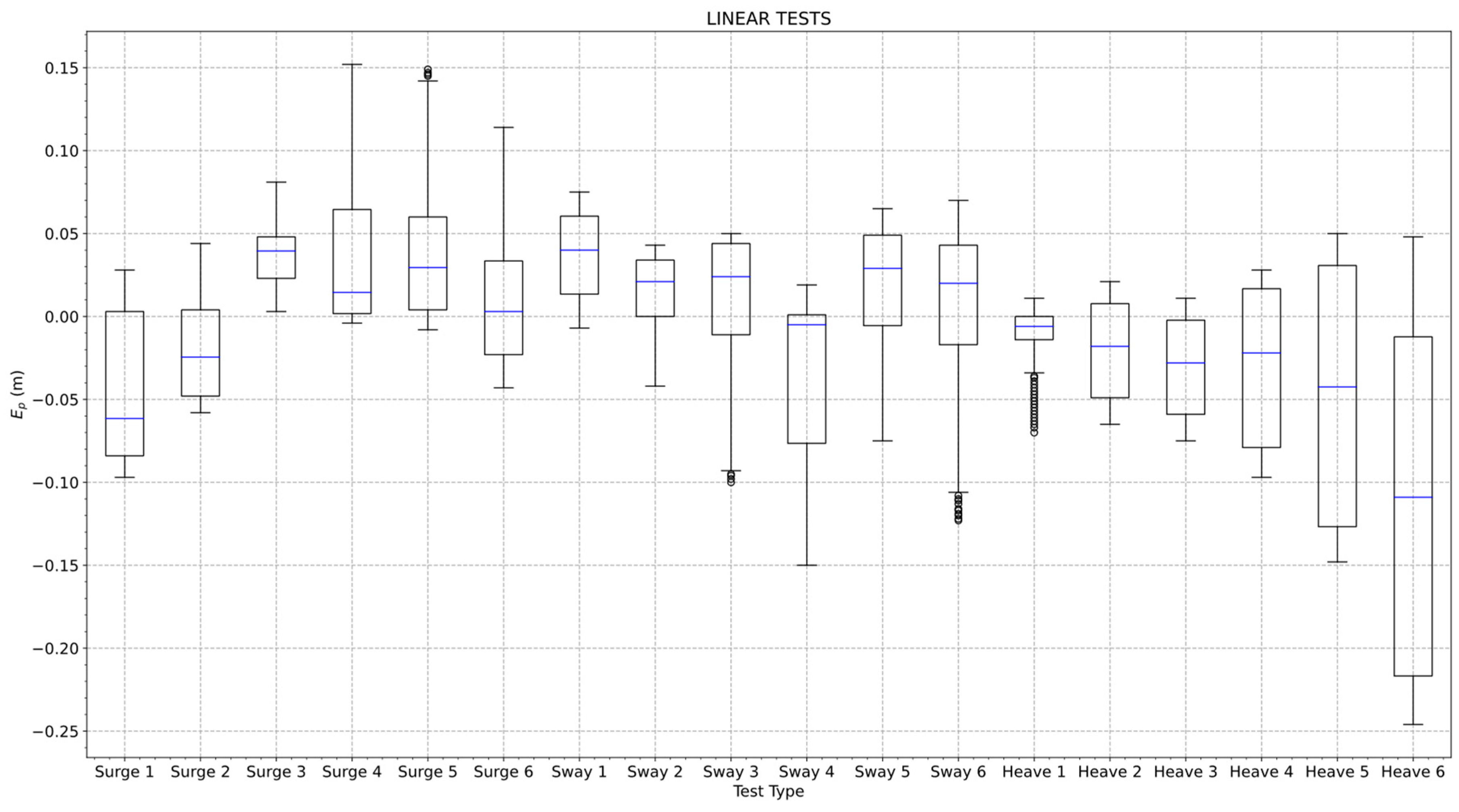
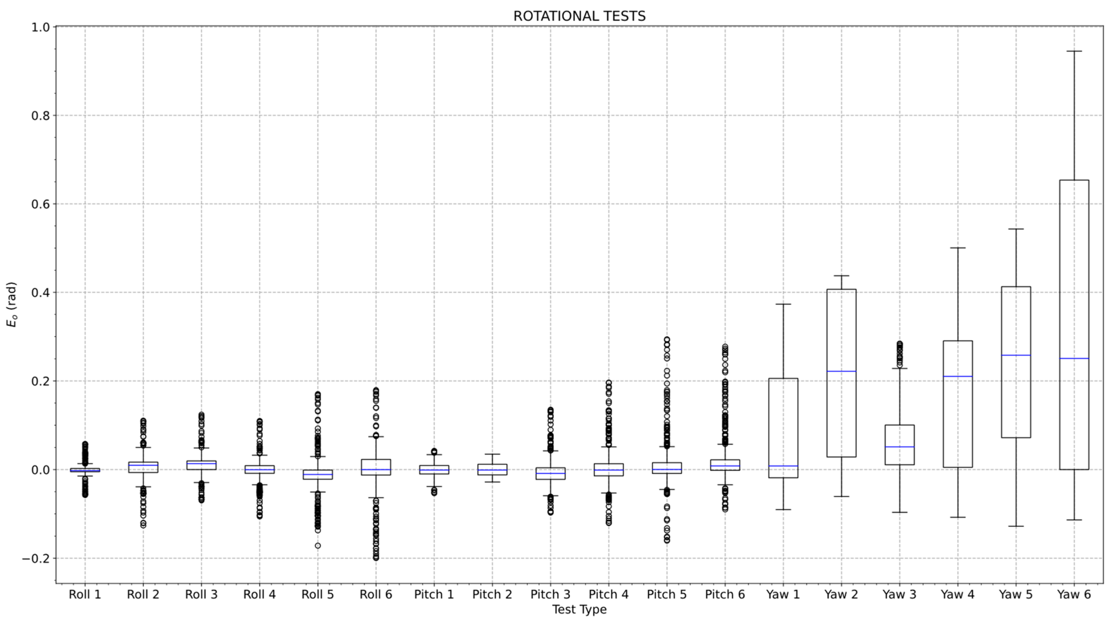
4.5. Analysis of the Results

Once the algorithm reached a solution, it was analyzed to verify that it was adequate and realistic. Some of this work was completed by setting an adequate range that avoided completely unrealistic solutions. The final values obtained are shown in

Table 5. Comparison between optimized and initial hydrodynamic coefficients for the BlueROV2.

Parameter	Initial Value	Optimized Value	Difference (%)
$I_{XX}$	0.344	0.371	7.85
$I_{YY}$	0.316	0.352	11.39
$I_{ZZ}$	0.389	0.426	9.51
$X_{\dot{u}}$	13.272	15.638	17.83
$Y_{\dot{v}}$	13.123	16.477	25.56
$Z_{\dot{w}}$	14.508	16.751	15.46
$K_{\dot{p}}$	0.207	0.157	−24.15
$M_{\dot{q}}$	0.211	0.165	−21.8
$N_{\dot{r}}$	0.109	0.133	22.02
$X_u$	−0.161	−0.153	−4.97
$Y_v$	−0.17	−0.176	3.53
$Z_w$	−0.254	−0.242	−4.72
$K_p$	−0.349	−0.377	8.02
$M_q$	−0.221	−0.201	−9.05
$N_r$	−0.141	−0.127	−9.93
$X_{u\left|u\right|}$	−33.346	−34.972	4.88
$Y_{v\left|v\right|}$	−45.731	−43.118	−5.71
$Z_{w\left|w\right|}$	−72.668	−70.209	−3.38
$K_{p\left|p\right|}$	−0.356	−0.389	9.27
$M_{q\left|q\right|}$	−0.461	−0.427	−7.38
$N_{r\left|r\right|}$	−0.471	−0.425	−9.77

.

The inertia values are very close to the initial estimations using the CAD model within a range of around 10%; however, the real values are slightly larger. This difference may well be caused by small elements that are not included in the CAD model, such as screws, cables, or similar objects. The added mass for the linear movements seems to be relatively close to the initial estimations but less accurate than the previous one, with a ±25% variation. Initial estimations for these values were intended to be only a general guide, so these results seem adequate. Regarding the physical meaning, results for the linear movements seem correct as the sway and heave movements that have a bigger surface area and tend to move more water with them show higher values of added mass. The rotational movements also seem correct, with values a little bit smaller than the initial estimations, but with a very similar relation between them.

The linear and quadratic damping coefficients for the displacements show very small variations within a ±5 range, which also confirms that the initial estimations with the load cell tests were accurate. Regarding the rotations, both linear and quadratic damping coefficients for the rotations show a higher difference in percentage, with the quadratic ones much closer to the estimations. It is important to consider that the values of these coefficients are small, so even small deviations from the original values are translated into big percentages. These results confirm that the hydrodynamic properties of the vehicle were kept after the optimization process and should improve the model’s behavior compared to the original one.

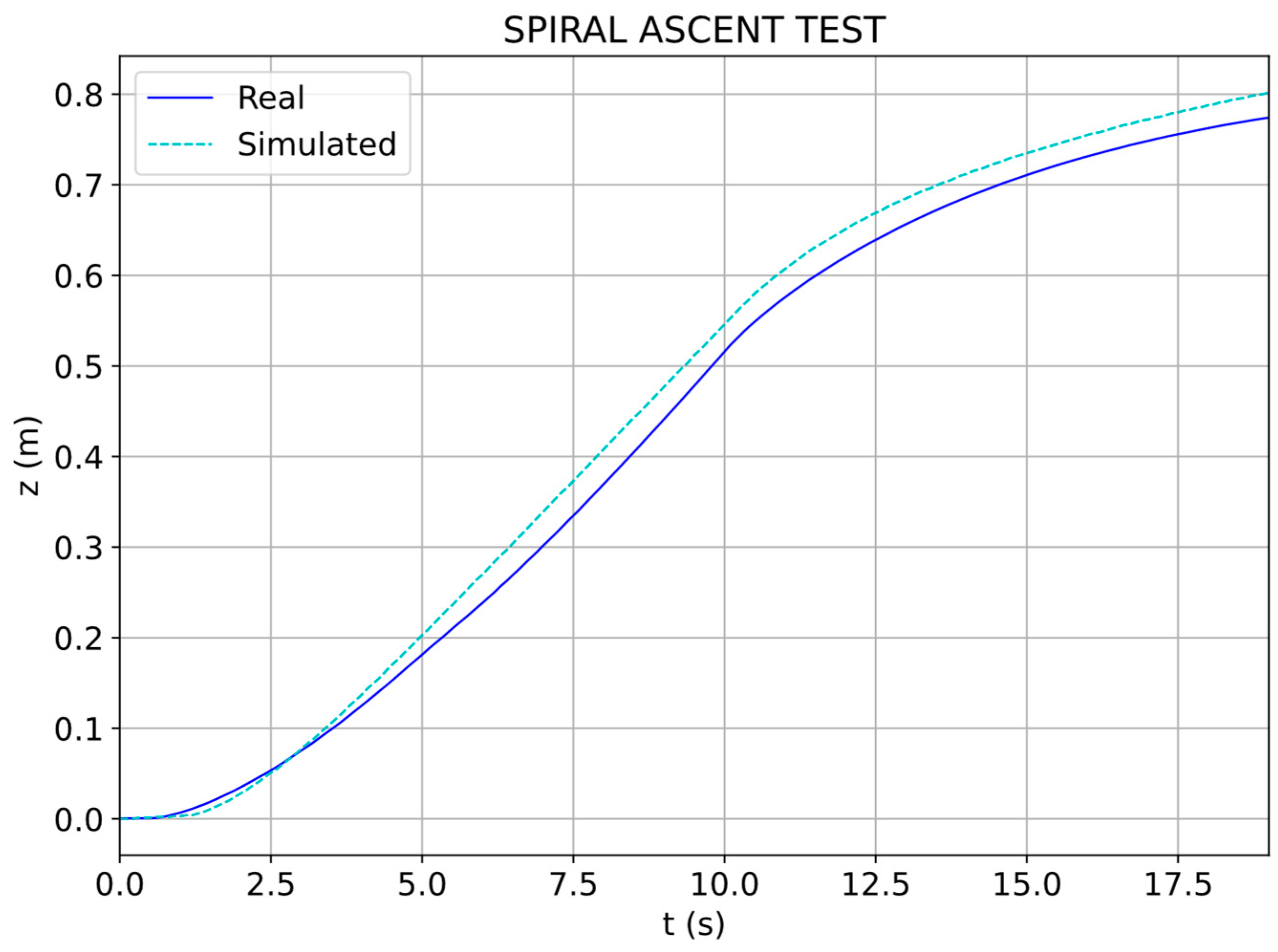
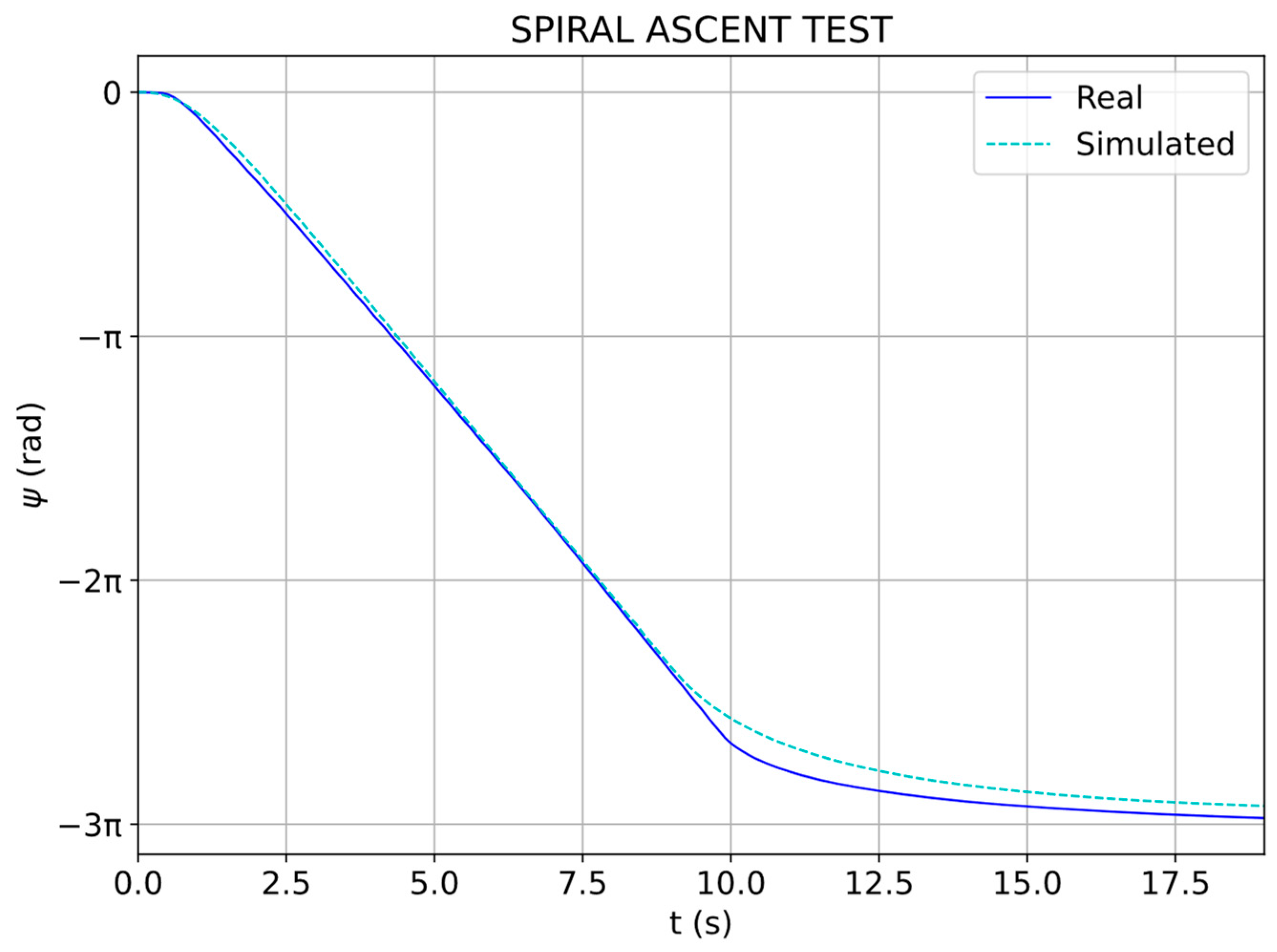
5. Digital Twin Model Validation

With the digital twin adjusted, a series of tests were performed to evaluate the effectiveness of the proposed solution. Figure 6 shows the position error (E_p) distribution for the linear validation tests, where the error values represent the difference between the real and simulated positions of the vehicle for each movement. Each group of boxplots corresponds to a specific linear motion: surge, sway, and heave. The tests consisted of six isolated movements along each axis, similar to those used during algorithm training, but with different amplitudes.

The amplitude ranges for the surge and sway motions were selected to ensure the robot exhibited representative behavior under typical operational conditions. In the case of heave motion, the range was limited by the depth of the towing tank. The results for the surge motion showed low error magnitudes, with most medians close to zero. This indicates that the simulated vehicle closely followed the trajectory of the real one. A similar trend was observed in the sway maneuvers, where the medians remained centered and the dispersion was moderate. The absence of a consistent trend in error magnitude with increasing amplitude suggests that the simulation accurately reproduced the vehicle’s behavior across the range of velocities tested.

The heave tests exhibited different behaviors. While the initial tests (Heave 1 to 3) followed a similar trend to the other linear motions, the remaining tests (Heave 4 to 6) showed significantly larger errors and variability. This discrepancy may be attributed to disturbances generated by the interaction between the fluid and the bottom of the towing tank, which appeared more pronounced at faster heave displacements.

Figure 7 shows the orientation error (E_o) distribution for the rotational validation tests where the error values represent the difference between the real and simulated orientations of the vehicle for each rotational movement. Each group of boxplots corresponds to a specific rotation (roll, pitch, and yaw). For roll and pitch, six tests were carried out up to the stability limit for the robot in these degrees of freedom. Beyond that point, the vehicle became unstable and tended to capsize, making it difficult to obtain reliable or repeatable results. In contrast, yaw rotations were tested over a wider propeller speed range, provided that the motion remained controllable and representative of real operational conditions, as high speeds in these tests did not compromise the robot’s stability.

The results for roll and pitch were consistent across all amplitudes, with low dispersion and median errors close to zero. This suggests a good match between the real and simulated responses for these two degrees of freedom. For yaw, the error values showed more variability, and the median was not centered around zero. This was expected, since the angular change in yaw was much larger than in roll or pitch, which naturally lead to a wider range of errors. Even so, the results followed a similar trend across the different test cases.

A detailed comparison of the angle over time for one of the pitch tests is presented in Figure 8. As can be seen, both the actuated and free motion behavior of the model were very close to the real vehicle. To further quantify the agreement, the root mean square error (RMSE) was computed, yielding a value of 0.015 and a normalized RMSE of 3.5%. These results indicate a strong correlation between the simulated and experimental data, suggesting that the model and the parameter optimization process are effective.

To validate the decoupled motion assumption and assess the model’s adequacy and generalization capability, a spiral ascent test was conducted. The results are illustrated in Figure 9 and Figure 10, which respectively compare the heave displacement and yaw angle over time, for both the real system and the simulation model. Both the heave displacement and the yaw evolution during the combined maneuver exhibited a high level of agreement between the real and simulated data, particularly during the actuated phase of the motion. Minor deviations observed in the latter part of the test can be attributed to unmodeled external effects, such as disturbances introduced by the tether or the discarded coupling effects.

The results, evidenced by the RMSE values of 0.03 (3.4%) for heave displacement and 0.17 (1.8%) for yaw angle, demonstrate that the model was capable of accurately capturing the translational and rotational dynamics independently, thus supporting the validity of the decoupling assumption made during model identification. Moreover, the ability to generalize to a complex, previously unseen trajectory involving simultaneous linear and rotational components highlights the model’s robustness and predictive reliability in nontrivial operational scenarios.

6. Conclusions

In this paper, a methodology to improve the hydrodynamic coefficients of an underwater vehicle is proposed. The methodology is based on the combination of an initial estimation using traditional methods, the application of evolutionary algorithms to refine it, and a critical analysis of the results. This approach could lead to more accurate hydrodynamic coefficient estimations.

The results of the validation tests reveal significant improvements in the accuracy of the position estimations by the simulator when using the optimized model as compared to the original one. The behavior of the optimized model is much closer to the real vehicle, offering a viable alternative solution to the use of CFD software to improve these parameters.

The validation tests also revealed that there is still a reality gap, showing some differences between the real and simulated vehicle, particularly in the transient response. These variations may be caused by some limitations of the mathematical model, which does not consider some known phenomena such as the coupling between different movements or the effects of the umbilical cord. However, the same methodology could be applied to more complex models if required.

References

1. Lee, G.M.; Park, J.Y.; Kim, B.; Baek, H.; Park, S.; Shim, H.; Choi, G.; Kim, B.R.; Kang, H.G.; Jun, B.H.; et al. Development of an autonomous underwater vehicle ISiMI6000 for deep-sea observation. Indian. J. Mar. Sci. 2013, 42, 8. [Google Scholar]
2. Rumson, A.G. The application of fully unmanned robotic systems for inspection of subsea pipelines. Ocean Eng. 2021, 235, 109214. [Google Scholar] [CrossRef]
3. Albiez, J.; Joyeux, S.; Gaudig, C.; Hilljegerdes, J.; Kroffke, S.; Schoo, C.; Arnold, S.; Mimoso, G.; Alcantara, P.; Saback, R.; et al. FlatFish—A compact subsea-resident inspection AUV. In Proceedings of the OCEANS 2015—MTS/IEEE, Washington, DC, USA, 19–22 October 2015. [Google Scholar] [CrossRef]
4. Wright, M.; Gorma, W.; Luo, Y.; Post, M.; Xiao, Q.; Durrant, A. Multi-actuated AUV Body for Windfarm Inspection: Lessons from the Bio-inspired RoboFish Field Trials. In Proceedings of the 2020 IEEE/OES Autonomous Underwater Vehicles Symposium, AUV 2020, St. Johns, NL, Canada, 30 September–2 October 2020. [Google Scholar] [CrossRef]
5. Martins, A.; Almeida, J.; Almeida, C.; Matias, B.; Kapusniak, S.; Silva, E. EVA a hybrid ROV/AUV for underwater mining operations support. In Proceedings of the 2018 OCEANS—MTS/IEEE Kobe Techno-Oceans, Kobe, Japan, 28–31 May 2018. [Google Scholar] [CrossRef]
6. AMartins, A.; Almeida, J.; Almeida, C.; Pereira, R.; Sytnyk, D.; Soares, E.; Matias, B.; Pereira, T.; Silva, E. MARA—A modular underwater robot for confined spaces exploration. In Proceedings of the 2020 Global Oceans 2020: Singapore—U.S. Gulf Coast, Biloxi, MS, USA, 5–30 October 2020. [Google Scholar] [CrossRef]
7. Kutzke, D.T.; Carter, J.B.; Hartman, B.T. Subsystem selection for digital twin development: A case study on an unmanned underwater vehicle. Ocean Eng. 2021, 223, 108629. [Google Scholar] [CrossRef]
8. Matsebe, O.; Kumile, C.M.; Tlale, N.S. A Review of Virtual Simulators for Autonomous Underwater Vehicles (AUVs). IFAC Proc. Vol. 2008, 41, 31–37. [Google Scholar] [CrossRef]
9. Cho, H.-S.; Sohn, J.-H.; Han, J.-B.; Yeu, T.-K. Development of a Real-Time Track Solver for Digital Twin of the Underwater Tracked Vehicle. Int. J. Precis. Eng. Manuf.-Green Technol. 2025, 12, 1023–1036. [Google Scholar] [CrossRef]
10. Ciuccoli, N.; Screpanti, L.; Scaradozzi, D. Underwater Simulators Analysis for Digital Twinning. IEEE Access 2024, 12, 34306–34324. [Google Scholar] [CrossRef]
11. Manhães, M.M.M.; Scherer, S.A.; Voss, M.; Douat, L.R.; Rauschenbach, T. UUV Simulator: A Gazebo-based package for underwater intervention and multi-robot simulation. In Proceedings of the OCEANS 2016 MTS/IEEE Monterey, OCE 2016, Monterey, CA, USA, 19–23 September 2016. [Google Scholar] [CrossRef]
12. Scaradozzi, D.; Gioiello, F.; Ciuccoli, N.; Drap, P. A Digital Twin Infrastructure for NGC of ROV during Inspection. Robotics 2024, 13, 96. [Google Scholar] [CrossRef]
13. Adetunji, F.O.; Ellis, N.; Koskinopoulou, M.; Carlucho, I.; Petillot, Y.R. Digital Twins Below the Surface: Enhancing Underwater Teleoperation. In Proceedings of the OCEANS 2024, Singapore, 15–18 April 2024; pp. 1–8. [Google Scholar] [CrossRef]
14. Wang, W.; Clark, C.M. Modeling and Simulation of the VideoRay Pro III Underwater Vehicle. In Proceedings of the OCEANS 2006—Asia Pacific, Singapore, 16–19 May 2006; pp. 1–7. [Google Scholar] [CrossRef]
15. Valeriano-Medina, Y.; Martínez, A.; Hernández, L.; Sahli, H.; Rodríguez, Y.; Cañizares, J.R. Dynamic model for an autonomous underwater vehicle based on experimental data. Math. Comput. Model. Dyn. Syst. 2013, 19, 175–200. [Google Scholar] [CrossRef]
16. Eidsvik, O.A.; Schjølberg, I. Time Domain Modeling of ROV Umbilical using Beam Equations. IFAC-PapersOnLine 2016, 49, 452–457. [Google Scholar] [CrossRef]
17. Satria, D.; Wiryadinata, R.; A Esiswitoyo, D.P.; I Adji, M.; Rosyadi, I.; Listijorini, E. Hydrodynamic analysis of Remotely Operated Vehicle (ROV) Observation Class using CFD. IOP Conf. Ser. Mater. Sci. Eng. 2019, 645, 012014. [Google Scholar] [CrossRef]
18. Zarei, A.; Ashouri, A.; Hashemi, S.M.J.; Bushehri, S.A.S.F.; Izadpanah, E.; Amini, Y. Experimental and numerical study of hydrodynamic performance of remotely operated vehicle. Ocean Eng. 2020, 212, 107612. [Google Scholar] [CrossRef]
19. Li, Q.; Cao, Y.; Li, B.; Ingram, D.M.; Kiprakis, A. Numerical Modelling and Experimental Testing of the Hydrodynamic Characteristics for an Open-Frame Remotely Operated Vehicle. J. Mar. Sci. Eng. 2020, 8, 688. [Google Scholar] [CrossRef]
20. Evans, J.; Nahon, M. Dynamics modeling and performance evaluation of an autonomous underwater vehicle. Ocean Eng. 2004, 31, 1835–1858. [Google Scholar] [CrossRef]
21. Kim, J.; Chung, W.K. Accurate and practical thruster modeling for underwater vehicles. Ocean Eng. 2006, 33, 566–586. [Google Scholar] [CrossRef]
22. Geisbert, J.S. Hydrodynamic Modeling for Autonomous Underwater Vehicles Using Computational and Semi-Empirical Methods. Ph.D. Thesis, Virginia Tech, Blacksburg, VA, USA, 2007. [Google Scholar]
23. Avila, J.P.J.; Adamowski, J.C. Experimental evaluation of the hydrodynamic coefficients of a ROV through Morison’s equation. Ocean Eng. 2011, 38, 2162–2170. [Google Scholar] [CrossRef]
24. Gabl, R.; Davey, T.; Cao, Y.; Li, Q.; Li, B.; Walker, K.L.; Giorgio-Serchi, F.; Aracri, S.; Kiprakis, A.; Stokes, A.A.; et al. Hydrodynamic loads on a restrained ROV under waves and current. Ocean Eng. 2021, 234, 109279. [Google Scholar] [CrossRef]
25. Fossen, T.I.; Fjellstad, O.-E. Nonlinear modelling of marine vehicles in 6 degrees of freedom. Math. Model. Syst. 1995, 1, 17–27. [Google Scholar] [CrossRef]
26. Lau, W.; Low, E.; Seet, G.; Chin, C. Estimation of the hydrodynamic coefficients of an ROV using free decay pendulum motion. Eng. Lett. 2008, 16, 326–331. [Google Scholar]
27. Avila, J.J.; Nishimoto, K.; Sampaio, C.M.; Adamowski, J.C. Experimental investigation of the hydrodynamic coefficients of a remotely operated vehicle using a planar motion mechanism. J. Offshore Mech. Arct. Eng. 2011, 134, 021601. [Google Scholar] [CrossRef]
28. Avila, J.P.J.; Donha, D.C.; Adamowski, J.C. Experimental model identification of open-frame underwater vehicles. Ocean Eng. 2013, 60, 81–94. [Google Scholar] [CrossRef]
29. Xie, S.; Li, Q.; Wu, P.; Luo, J.; Li, F.; Gu, J. Hydrodynamic coefficients identification and experimental investigation for an underwater vehicle. Sens. Transducers 2014, 164, 81–94. [Google Scholar]
30. Eidsvik, O.A. Identification of Hydrodynamic Parameters for Remotely Operated Vehicles. Master’s Thesis, Norwegian University of Science and Technology, Trondheim, Norway, 2015. [Google Scholar]
31. Eidsvik, O.A.; Schjølberg, I. Determination of hydrodynamic parameters for remotely operated vehicles. In Proceedings of the International Conference on Offshore Mechanics and Arctic Engineering—OMAE, Busan, Republic of Korea, 19–24 June 2016. [Google Scholar] [CrossRef]
32. Lee, Y.; Lee, Y.; Chae, J.; Choi, H.T.; Yeu, T.K. Preliminary Experiments to Determine Hydrodynamic Coefficients of Remotely Operated Vehicle. In Proceedings of the OCEANS 2019—Marseille, Marseille, France, 17–20 June 2019. [Google Scholar] [CrossRef]
33. Hammoud, A.; Sahili, J.; Madi, M.; Maalouf, E. Design and dynamic modeling of ROVs: Estimating the damping and added mass parameters. Ocean Eng. 2021, 239, 109818. [Google Scholar] [CrossRef]
34. Rojas, J.; Eichhorn, M.; Baatar, G.; Matz, S.; Glotzbach, T. Parameter Identification and Optimization of an Oceanographic Monitoring Remotely Operated Vehicle. In Proceedings of the 2018 OCEANS—MTS/IEEE Kobe Techno-Oceans, Kobe, Japan, 28–31 May 2018. [Google Scholar] [CrossRef]
35. Soliman, M.A. Estimation of the ROV hydrodynamic coefficients using CFD. Int. Undergrad. Res. Conf. 2022, 6, 1–8. [Google Scholar]
36. Panda, J.P.; Mitra, A.; Warrior, H.V. A review on the hydrodynamic characteristics of autonomous underwater vehicles. J. Eng. Marit. Environ. 2020, 235, 15–29. [Google Scholar] [CrossRef]
37. Lack, S.; Rentzow, E.; Jeinsch, T. Experimental Parameter Identification for an open-frame ROV: Comparison of towing tank tests and open water self-propelled tests. IFAC-Pap. 2019, 52, 271–276. [Google Scholar] [CrossRef]
38. Busse, C.; Reich, J.E.; Renner, B.C. In Situ Damping Parameter Estimation for an Underwater Vehicle Using Onboard Sensors. In Proceedings of the 2022 IEEE/OES Autonomous Underwater Vehicles Symposium, Singapore, 19–21 September 2022. [Google Scholar] [CrossRef]
39. von Benzon, M.; Sørensen, F.F.; Uth, E.; Jouffroy, J.; Liniger, J.; Pedersen, S. An Open-Source Benchmark Simulator: Control of a BlueROV2 Underwater Robot. J. Mar. Sci. Eng. 2022, 10, 1898. [Google Scholar] [CrossRef]
40. Goldberg, D.E. Genetic and Evolutionary Algorithms Come of Age. Commun. ACM 1994, 37, 113–119. [Google Scholar] [CrossRef]
41. Rodriguez-Cortegoso, J.; Romero, A.; Orjales, F.; Deibe, A.; Diaz-Casas, V. Improving the Hydrodynamic Characterization of Autonomous Underwater Vehicles Through Deep Learning. In Proceedings of the The 33rd International Ocean and Polar Engineering Conference, Ottawa, ON, Canada, 19–23 June 2023; pp. 1764–1769. [Google Scholar]
42. Koenig, N.; Howard, A. Design and use paradigms for Gazebo, an Open-Source Multi-Robot Simulator. In Proceedings of the 2004 IEEE/RSJ International Conference on Intelligent Robots and Systems (IROS), Sendai, Japan, 28 September–2 October 2004. [Google Scholar] [CrossRef]
43. Fossen, T.I. Handbook of Marine Craft Hydrodynamics and Motion Control; Wiley: Hoboken, NJ, USA, 2021. [Google Scholar] [CrossRef]
44. Hydromechanics Subcommittee of the Technical and Research Committee of the Society of Naval Architects and Marine Engineers. SNAME, Nomenclature for Treating the Motion of a Submerged Body Through a Fluid; The Society of Naval Architects and Marine Engineers: New York, NY, USA, 1950; pp. 1–5. [Google Scholar]
45. Antonelli, G. Underwater Robots; Springer International Publishing: Cham, Switzerland, 2014; Volume 96. [Google Scholar] [CrossRef]
46. Lam, J.; Chen, A.; Bennett, A.; Triantafyllou, M. Propeller Characterization Testing of a Blue Robotics T200 Thruster. In Proceedings of the OCEANS 2023—Limerick, Limerick, Ireland, 5–8 June 2023; pp. 1–8. [Google Scholar] [CrossRef]
47. Fortin, F.A.; De Rainville, F.M.; Gardner, M.A.; Parizeau, M.; Gagńe, C. DEAP: Evolutionary algorithms made easy. J. Mach. Learn. Res. 2012, 13, 2171–2175. [Google Scholar]
Figure 1. Methodology process diagram.
Applsci 15 07085 g001
Figure 2. BlueROV2 prepared for tests.
Applsci 15 07085 g002
Figure 3. Estimated and measured thruster curve for surge movement.
Applsci 15 07085 g003
Figure 4. Setup for motion capture system.
Applsci 15 07085 g004
Figure 5. Block diagram illustrates the flow of the proposed genetic algorithm.
Applsci 15 07085 g005
Figure 6. Error in the linear validation tests: 6 for surge, 6 for sway, and 6 for heave.
Applsci 15 07085 g006
Figure 7. Error in the rotational validation tests: 6 for roll, 6 for pitch, and 6 for yaw.
Applsci 15 07085 g007
Figure 8. Pitch angle evolution over time in one of the pitch validation tests for the simulated and real vehicle.
Applsci 15 07085 g008
Figure 9. Heave displacement during spiral ascent test.
Applsci 15 07085 g009
Figure 10. Yaw evolution during spiral ascent test.
Applsci 15 07085 g010