Integration of RSM and Machine Learning for Accurate Prediction of Surface Roughness in Laser Processing

Featured Application

The proposed hybrid modeling approach, combining response surface methodology and regression tree learning, can be effectively applied to improve prediction accuracy in laser machining processes. It is particularly useful in industrial settings, where precise control of surface roughness is critical.

Abstract

This study investigates the modeling of surface roughness (Ra) in the laser cutting of EN 10130 steel process by integrating classical statistical and machine learning methods. First, a quadratic model was developed using response surface methodology (RSM) based on a Box–Behnken experimental design with 17 runs, using cutting speed, laser power, and auxiliary gas pressure as input parameters. Although the RSM model achieved an R² value of 0.8227, there were still some nonlinear deviations between the predicted and experimental values. To improve the prediction accuracy, a regression tree algorithm was applied to model the residuals of the RSM output. The resulting hybrid model, which combines RSM predictions with machine learning-based corrections, yielded a higher R² of 0.8889 and a lower RMSE compared to the original RSM model. A leave-one-out cross-validation (LOOCV) was performed to evaluate the generalization, which resulted in an RMSE of 0.3241 and an R² of 0.6039. These findings confirm the effectiveness of the hybrid approach in capturing complex dependencies and improving prediction accuracy, highlighting its potential for advanced process modeling in laser machining.

1. Introduction

Laser cutting has become a fundamental technology in modern manufacturing due to its ability to deliver high precision and process a wide range of materials, including metals, polymers, and fiber-reinforced composites [1]. Despite these advantages, the industry is increasingly demanding tighter tolerances and better surface finishes. As a result, surface roughness (Ra) has become an important quality indicator, as it affects not only the aesthetic appeal but also the functional performance of components [2]. Even though laser cutting is a well-established technology, achieving good surface quality remains a challenge due to the complex and often nonlinear interactions between process parameters. For example, certain combinations of cutting speed and laser power can cause chaotic melt ejection [3,4,5]. Additional issues include gas pressure instabilities and material damage caused by overheating and resolidification [6]. These subtleties highlight the need for advanced modeling strategies capable of capturing the underlying physics while supporting robust process optimization.

Response surface methodology (RSM) is often used to develop empirical models that describe the relationship between input process parameters and output performance metrics. For example, Shrivastava et al. successfully applied a Box–Behnken RSM design to optimize surface roughness (Ra) and kerf width in the laser cutting of Inconel 718 sheets [7]. Their regression models demonstrated high predictive accuracy, with an R² value of approximately 99%, identifying cutting speed and laser power as the most influential factors affecting cut quality. Wang et al. used RSM to develop quadratic models based on four input process parameters—oxygen pressure, pulse width, pulse frequency, and cutting speed—and two output responses: average kerf taper and surface roughness (Ra) [8]. The analysis of variance (ANOVA) results indicated good agreement between the experimental data and the predicted nonlinear regression model, with R² values of approximately 97%. Similarly, Boudjemline et al. developed a multiple linear regression model to predict the maximum surface roughness height in CO₂ laser cutting of Ti-6Al-4V alloys [9]. Their analysis showed that the cutting speed was the dominant factor for surface roughness, while the auxiliary gas pressure had a negligible influence within the investigated range. The model was validated using ANOVA and achieved a high coefficient of determination (R²) of 99.33%, confirming its appropriateness. Similarly, Ming systematically investigated the effects of process parameters, such as cutting speed, focal length, and laser power, on the temperature adjacent to the cut kerf and cutting surface roughness using RSM [10]. A central composite design (CCD) was employed for the experimental setup and ANOVA, which revealed the significance of each factor’s contribution to the responses. The resulting regression models demonstrated high accuracy in predicting both temperature distribution and surface roughness. Generally, these studies affirm RSM’s value as a transparent and statistically sound tool for surface quality prediction in laser-based manufacturing processes. It is worth noting, however, that these models were developed using relatively large experimental datasets, which likely contributed to the high R² values.

Recent advances in machine learning (ML) have enabled highly accurate modeling of surface roughness in laser cutting processes, often more successfully traditional statistical approaches in predictive performance. Kusuma and Huang evaluated the performance of three machine learning models—support vector regression, random forest, and extreme learning machine—for predicting kerf width in pulsed laser cutting [11]. They indicated that the vibration features selected from the optimal base wavelet selection combined with the random forest model are efficient for forecasting the straight kerf width of the workpiece by pulsed laser cutting. Tercan et al. proposed a hybrid machine learning approach that combines clustering and classification to support laser cutting process planning by extracting meaningful patterns from time-consuming simulation data [12]. Their method enables designers to identify key parameter regions associated with high-quality cuts and gain valuable insights through interpretable models and visualization techniques. Chen et al. developed predictive models using decision trees, random forests, and support vector machines for surface roughness in the fiber laser cutting of aluminum, based on 81 experimental points [13]. Among the tested algorithms, the random forest model achieved the best performance, with an R² of 0.981 and RMSE of 0.206, outperforming support vector regression (R² = 0.959, RMSE = 0.298) and gradient boosting (R² = 0.968, RMSE = 0.260). Tianhao et al. proposed a high-precision roughness prediction model for high-power laser bevel cutting based on a least-squares support vector machine augmented by a whale optimization algorithm [14]. The optimized model achieves a reasonable coefficient of determination of 0.9576 and shows great potential for the effective prediction of bevel surface roughness. These developments underscore the growing role of machine learning in predicting laser processing performance characteristics. Despite its predictive power, full industrial adoption remains limited. This is because of the transparency of the methods and explainability. Most importantly, studies to date have relied predominantly on purely data-driven machine learning models, without considering the underlying physical or mathematical relationships.

Several critical gaps in the current literature motivate the development of a hybrid RSM–ML framework, which is particularly suitable for applications with limited datasets. First, stand-alone RSM models are often unable to capture the nonlinear behavior of modern manufacturing processes. For example, Bose and Nandi highlighted the limitations of RSM in modeling complex interactions in wire EDM of hybrid titanium–matrix composites, suggesting that RSM alone may not provide sufficient accuracy in such complicated processes [15]. Similarly, comprehensive reviews emphasized the shortcomings of RSM in high-dimensional and nonlinear problem spaces, advocating the integration of intelligent algorithms to enhance modeling flexibility and accuracy [16,17]. Secondly, integrating RSM with ML techniques has shown promise in enhancing predictive accuracy. Gao et al. demonstrated that a hybrid model combining RSM with a whale optimization algorithm-optimized back-propagation neural network outperformed traditional RSM in optimizing laser-induced hybrid hardening processes, indicating the efficacy of such hybrid approaches in capturing complex process dynamics [18]. These findings align with those in the review by Piri et al., who observed that hybrid RSM–ML models consistently deliver better performance in process optimization across various advanced manufacturing domains [19]. Finally, rigorous validation strategies are essential to ensure the generalizability of prediction models [20,21]. Leave-one-out cross-validation is widely used in structural optimization and reliability analysis, as it provides nearly unbiased error estimates especially useful for small datasets [22]. However, the aforementioned method can be very computationally intensive. To overcome this, improved leave-one-out cross-validation techniques have been developed that incorporate hyperparameter tuning from the full training dataset to improve both the accuracy and efficiency of model evaluation [23].

This study presents a hybrid RSM–ML framework for predicting the surface roughness of laser-cut EN 10130 steel. By integrating the interpretability of the RSM with regression tree-based residual correction, the framework achieves significantly improved prediction accuracy. The modeling process begins with the development of a quadratic RSM model, which is refined by eliminating statistically nonsignificant terms. The residuals are then modeled using regression trees, effectively capturing nonlinear effects that were not considered in the original RSM formulation.

To ensure the robustness and generalizability of the model, verification is performed using leave-one-out cross-validation (LOOCV), a step that is often overlooked in similar studies. The proposed workflow offers a balanced approach that combines the transparency of RSM with the enhanced predictive capability of machine learning, providing a practical and adaptable solution for industrial applications where both model accuracy and interpretability are essential.

The paper is structured as follows: Section 2 describes the materials used, the methodology, and the experimental setup. Section 3 offers a discussion of the obtained results, their implications, and potential directions for future research. Finally, Section 4 summarizes the main conclusions and key findings of the study.

2. Materials and Methods

In this study, a hybrid modeling strategy was employed by combining the classical response surface methodology (RSM) with machine learning (ML). The RSM approach was applied to develop a regression model based on the Box–Behnken experimental design. Residuals between the experimental and predicted values of surface roughness were subsequently modeled using the regression tree algorithm (fitrtree). This enabled the correction of systematic deviations and improved the accuracy of the predictions. The final model combines RSM predictions with ML-based residual corrections, offering enhanced adaptability to nonlinear behavior. The process is illustrated in Figure 1.

2.1. Description of Experimental Setup

The experimental tests were carried out using a Glorystar GS4020 (Glorystar Laser Technology Co., Ltd., Dongguan, China) fiber laser cutting machine with a maximum laser power of 1.5 kW. This machine ensures high cutting precision and stability and is therefore suitable for processing various types of metal sheets.

The material used in this study was cold-rolled low-carbon steel of grade EN 10130, which is widely used in various industries due to its excellent surface finish and dimensional stability. The sheet thickness used for the experiments was 5 mm. During the laser process, the cutting speed, laser power, and gas pressure were varied. The laser power was set within a certain percentage of the maximum machine power (1.5 kW), while the cutting speed was selected to ensure efficient material separation and minimal thermal deformation. Oxygen was used as an auxiliary gas. The selected cutting modes are listed in

Table 1. Parameters and their levels during laser cutting.

Factor	A	B	C
Cutting speed [m/min]	0.9	1.1	1.3
Laser power [%]	80	84	88
Gas pressure [bar]	1	1.1	1.2

.

An illustration of a steel sheet cutting experiment is presented in Figure 2. In all experiments, various laser cutting parameters were kept constant to ensure process stability and repeatability. Oxygen was used as the auxiliary gas, and a constant nozzle configuration with a double nozzle of 1.5 mm diameter was used. The cutting height was maintained at 0.7 mm, while the laser frequency was set to 5000 Hz. The laser focus position was set at −3.8 mm and the focus setting of the device was kept at +2.6. These parameters were chosen based on manufacturer recommendations to ensure consistent cutting conditions across all trials.

The surface roughness was evaluated with the average roughness parameter Ra, which was measured with a Mitutoyo Surftest SJ-210 (Mitutoyo Corporation, Kawasaki, Japan). The laser-cut surface usually consists of three different zones: the initial entry zone that occurs when the laser beam penetrates the material, a smooth zone that results from a stable cut, and a rough zone at the bottom, where the roughness is most pronounced. In this study, the width of the rough zone was used as a key indicator of cut quality, as it is the most sensitive to irregularities during processing. The roughness measurements were taken in the middle of this rough zone (Figure 3).

2.2. Box–Behnken Design

To investigate the effect of input parameters on surface roughness during laser cutting, a Box–Behnken design was used. This design is considered highly efficient, as it enables the development of a mathematical model and the assessment of parameter influence while minimizing the number of experiments, resulting in significant savings in both time and cost. The experimental results obtained in terms of surface roughness are shown in

Table 2. Experimental results of surface roughness evaluation for the Box–Behnken design.

	Code Factors				Input Factors			Outputs
No.	x0	x1	x2	x3	v [m/min]	Pw [%]	P [bar]	Ra (µm)	Ra RSM (µm)	Residual (-)	Ra HYB (µm)
1.	1	−1	−1	0	0.90	80.00	1.10	3.151	3.073	0.078	3.071
2.	1	1	−1	0	1.30	80.00	1.10	3.994	3.677	0.317	4.011
3.	1	−1	1	0	0.90	88.00	1.10	2.541	2.628	−0.087	2.480
4.	1	1	1	0	1.30	88.00	1.10	2.951	3.232	−0.281	3.084
5.	1	−1	0	−1	0.90	84.00	1.00	2.399	2.366	0.033	2.315
6.	1	1	0	−1	1.30	84.00	1.00	2.585	2.970	−0.385	2.919
7.	1	−1	0	1	0.90	84.00	1.20	2.342	2.366	−0.024	2.364
8.	1	1	0	1	1.30	84.00	1.20	3.320	2.970	0.350	3.304
9.	1	0	−1	−1	1.10	80.00	1.00	2.493	2.789	−0.296	2.738
10.	1	0	1	−1	1.10	88.00	1.00	2.787	2.344	0.443	2.293
11.	1	0	−1	1	1.10	80.00	1.20	2.69	2.789	−0.099	2.787
12.	1	0	1	1	1.10	88.00	1.20	2.269	2.344	−0.075	2.196
13.	1	0	0	0	1.10	84.00	1.10	1.964	2.082	−0.118	2.080
14.	1	0	0	0	1.10	84.00	1.10	2.025	2.082	−0.057	2.080
15.	1	0	0	0	1.10	84.00	1.10	2.159	2.082	0.077	2.080
16.	1	0	0	0	1.10	84.00	1.10	2.188	2.082	0.106	2.080
17.	1	0	0	0	1.10	84.00	1.10	2.099	2.082	0.017	2.080

.

2.3. Response Surface Methodology

Response surface methodology (RSM) is a collection of statistical and mathematical techniques used to model and optimize the relationship between multiple input variables (factors) and a response (output). It is often used in process optimization, design of experiments (DoE), and predictive modeling. RSM usually involves the design of experiments (e.g., central composite design, Box–Behnken design) and the fitting of a regression model (usually a linear or quadratic model). The main objective of this method is to analyze the response surface to find optimal conditions.

Since surface roughness after laser cutting exhibits nonlinear behavior, it is necessary to develop nonlinear prediction models to achieve the best correlation between the predicted and experimental results. The RSM was used to represent the relationship between the input parameters and the output parameters, as shown in Equation (1).

$$Y=f\left(v, P_w, P\right)+error$$

(1)

In this study, experimental errors are evaluated through residuals, and the response Y is modeled using a quadratic polynomial multiple regression (Equation (2)).

$$Y=c_0+\sum _{i=1}^3{c}_i{x}_i+\sum _{i=1}^3{c}_{ii}{x}_i^2+\sum _{i<j}^3{c}_{ij}{x}_i{x}_j$$

(2)

Here, c₀ is the constant term, while c_i, c_ii, and c_ij represent the coefficients of the linear, quadratic, and interaction terms, respectively. Using cutting speed (v), laser power (P_w), and assist gas pressure (P) as the three input parameters, the surface roughness response Y can be expressed by Equation (3).

$$Y=c_0+c_{1}v+c_2{P}_w+c_{3}P+c_{11}{v}^2+c_{22}{P}_w^2+c_{33}{P}^2+c_{12}v{P}_w+c_{13}vP+c_{23}{P}_{w}P$$

(3)

2.4. Machine Learning Method—Decision Tree Regression

Decision tree regression (DTR) is a nonparametric supervised learning method used for predicting continuous outcomes by recursively partitioning the feature space. Unlike parametric approaches such as response surface methodology (RSM), which rely on predefined polynomial functions, DTR adaptively splits data into subgroups to minimize prediction error. In this study, DTR is employed to model and correct the residuals of the discrepancies between experimental measurements (R_aexp) and RSM-predicted values (R_arsm). Since RSM may not fully capture complex nonlinear relationships in the data, DTR enhances predictive accuracy by learning the underlying patterns in these residuals.

The splitting process in DTR is governed by impurity reduction, typically measured using mean squared error (MSE). At each node, the algorithm evaluates potential splits across all features and thresholds, selecting the one that maximizes the decrease in MSE. The MSE for a given node is calculated as the average squared difference between the observed values and their mean within that node (Equation (4)):

$$MSE={\displaystyle \frac{1}{n}}\sum _{i=1}^n{(y_i-\overline{y})}^2$$

(4)

where n represents the number of samples in the node, y_i denotes the actual response value, and $\overline{y}$ is the mean response of the node. The quality of a split is quantified by the reduction in MSE (ΔMSE), computed as the difference between the parent node’s MSE and the weighted MSE of its child nodes (Equation (5)):

$$\Delta MSE={MSE}_{parent}-(w_L·{MSE}_L+w_R·{MSE}_R)$$

(5)

where ${MSE}_{parent}$ is the MSE before the split, ${MSE}_L$ and ${MSE}_R$ are the MSE values for the left and right child nodes, and $w_L$ and $w_R$ are the proportions of samples in the left and right nodes.

To prevent overfitting, tree growth is constrained by stopping criteria such as the maximum number of splits (MaxNumSplits), minimum samples per leaf node, or a minimum improvement in impurity. These parameters control the model’s complexity, balancing bias and variance. By integrating DTR-corrected residuals with RSM predictions (Equation (6)),

R_ahybrid = R_arsm + Residual,

(6)

the hybrid model achieves superior accuracy, particularly in capturing nonlinearities that the RSM alone might miss. This approach combines the interpretability of RSM with the flexibility of machine learning, offering a robust framework for predictive modeling.

3. Results and Discussion

3.1. Development of the RSM Model

For the purposes of this study, laser cutting experiments were designed using a Box–Behnken experimental design with three factors at three levels. The independent variables were cutting speed (A), laser power (B), and assist gas pressure (C). The dependent variable, or system response, was surface roughness. Initially, the significance of the model and its terms was determined through analysis of variance (ANOVA). Based on the statistical evaluation of the model’s adequacy and the significance of deviations from the model, a quadratic model was recommended for surface roughness and subsequently selected for further analysis. A backward elimination method was applied to remove nonsignificant terms, resulting in a reduced model containing only influential parameters.

Table 3. ANOVA for response surface reduced quadratic model.

Source	Sum of Squares	df	Mean Square	F Value	p-Value	Significance
Model	3.71	4	0.93	13.93	0.0002	Significant
A-v	0.73	1	0.73	10.96	0.0062	None
B-Pw	0.4	1	0.4	5.95	0.0313	None
A2	1.45	1	1.45	21.79	0.0005	None
B2	0.99	1	0.99	14.88	0.0023	None
Residual	0.8	12	0.067	None	None	None
Lack of Fit	0.76	8	0.096	11.08	0.0171	Significant
Pure Error	0.035	4	0.008626	None	None	None
Cor Total	4.51	16	None	None	None	None

presents the reduced ANOVA table with the significant factors retained.

The analysis of variance (ANOVA) indicated that the developed model is statistically significant, with a model F-value of 13.93 and only a 0.02% probability that such a high F-value could occur due to noise.

Factors A and B, as well as their quadratic terms (A² and B²), were found to be significant (p-values less than 0.05), while factor C was excluded from the model due to its lack of statistical significance, according to the RSM analysis. Since the inclusion of nonsignificant terms can degrade model quality, a model reduction was performed to enhance predictive performance and simplify interpretation.

The lack of fit test revealed a significant mismatch between the model and the experimental data (lack of fit F-value of 11.08, p = 0.0171), suggesting that the model does not fully capture the variability in the response and could be further improved.

The reduced model, obtained by eliminating nonsignificant factors, will be used for further process optimization and prediction of surface roughness during laser processing. Its improved simplicity and maintained statistical significance make it suitable for reliable interpretation and practical application. The final model, in terms of actual factors, is given in Equation (7):

$$R_a=236.534-30.738·v-5.143·P_w+14.658·v^2+0.030·P_w^2$$

(7)

The basic statistical data of the reduced quadratic model for processing productivity are presented in

Table 4. Basic statistical data of the adopted model.

Statistic	Value	Statistic	Value
Std. Dev.	0.26	R-Squared	0.8227
Mean	2.59	Adj R-Squared	0.7637
C.V. %	9.98	Pred R-Squared	0.5898
PRESS	1.85	Adeq Precision	11.399

. The coefficient of determination (R-squared) is 0.8227, indicating a strong relationship between the model predictions and experimental data. Both the adjusted R-squared (0.7637) and the predicted R-squared (0.5898) are reasonably close to each other, which confirms the significance and reliability of the model. The adequacy of the model is further supported by the Adeq Precision value of 11.399, which is well above the recommended minimum of 4, indicating an adequate signal-to-noise ratio. In addition, the coefficient of variation (C.V. %) of 9.98% and the predicted residual sum of squares (PRESS) value of 1.85 further confirm the model’s significance and stability.

3.2. Influence of Input Parameters on Surface Roughness

The influence of each process parameter on surface roughness (Ra) was further analyzed using a perturbation diagram, which illustrates the effects of changing one factor at a time while keeping the others at their central values. As can be seen in Figure 4, cutting speed (A) has the greatest influence on Ra, followed by laser power (B), while auxiliary gas pressure (C) has a relatively small influence. The dominant influence of cutting speed can be attributed to the phenomenon of melt jet retardation at higher speeds, where the interaction between the molten material and the assist gas is less effective. This delay can lead to incomplete material removal and an increase in surface roughness. Laser power also has a significant impact on Ra, as more energy enters the cutting zone at higher power, increasing the amount of molten material and potentially creating a rougher surface if it is not ejected properly. Although gas pressure showed a limited impact on surface roughness within the experimental range, its presence remains essential for maintaining cut quality. It facilitates the efficient removal of molten material and prevents dross formation, contributing to cleaner and more stable cutting conditions.

To complement the qualitative analysis of the perturbation diagram (Figure 4), a quantitative sensitivity analysis is presented in Figure 5. The contribution of each significant factor from the reduced RSM model was calculated based on the normalized sum of squares from the ANOVA. As can be seen from the bar chart, the quadratic term A² (cutting speed squared) had the greatest influence on surface roughness, contributing approximately 40.6%, followed by B² (laser power squared) at 27.7%, A (cutting speed) at 20.4%, and B (laser power) at 11.2%.

These contributions reflect the nonlinear and dominant role of cutting speed in the laser cutting process. The strong influence of A² indicates that both too low and too high cutting speeds can deteriorate the surface finish, probably due to the instability of the melt pool and insufficient material removal. Similarly, the influence of B² suggests that the surface roughness also depends on the fine-tuning of the laser power: too low a power leads to incomplete cutting, while too high a power increases the molten material, causing rougher surfaces. The lower contribution of B confirms its secondary but nevertheless important role in the energy balance of the process.

3.3. Residual Modeling Using Regression Trees

The RSM model provided a statistically significant fit and revealed the key influences of individual process parameters on surface roughness. However, deviations between predicted and experimental values remained, with a coefficient of determination (R²) of 0.8227 and a root mean square error (RMSE) of 0.2169, indicating that further improvement in predictive accuracy was possible.

To address these residual discrepancies and capture nonlinearities not modeled by quadratic regression, a residual modeling approach using regression trees was implemented. Rather than predicting surface roughness directly, the algorithm was trained on residuals defined in Equation (6), representing the differences between experimental and RSM-predicted values.

This residual-based modeling strategy was chosen because the RSM model had already captured the dominant linear and quadratic trends. By applying regression trees only to the residuals, the model focused on identifying the remaining nonlinear structures, thereby reducing the risk of overfitting and preserving model interpretability.

The dataset consisted of 17 samples obtained from a Box–Behnken design, with cutting speed, laser power, and assist gas pressure as input variables. A grid search was conducted by varying the MaxNumSplits parameter from 1 to 10 to determine the optimal tree complexity. The best results were achieved with MaxNumSplits = 3, yielding a minimum RMSE of 0.1717. This indicates that a moderately complex regression tree was sufficient to capture the residual structure without overfitting a crucial consideration, given the limited number of samples.

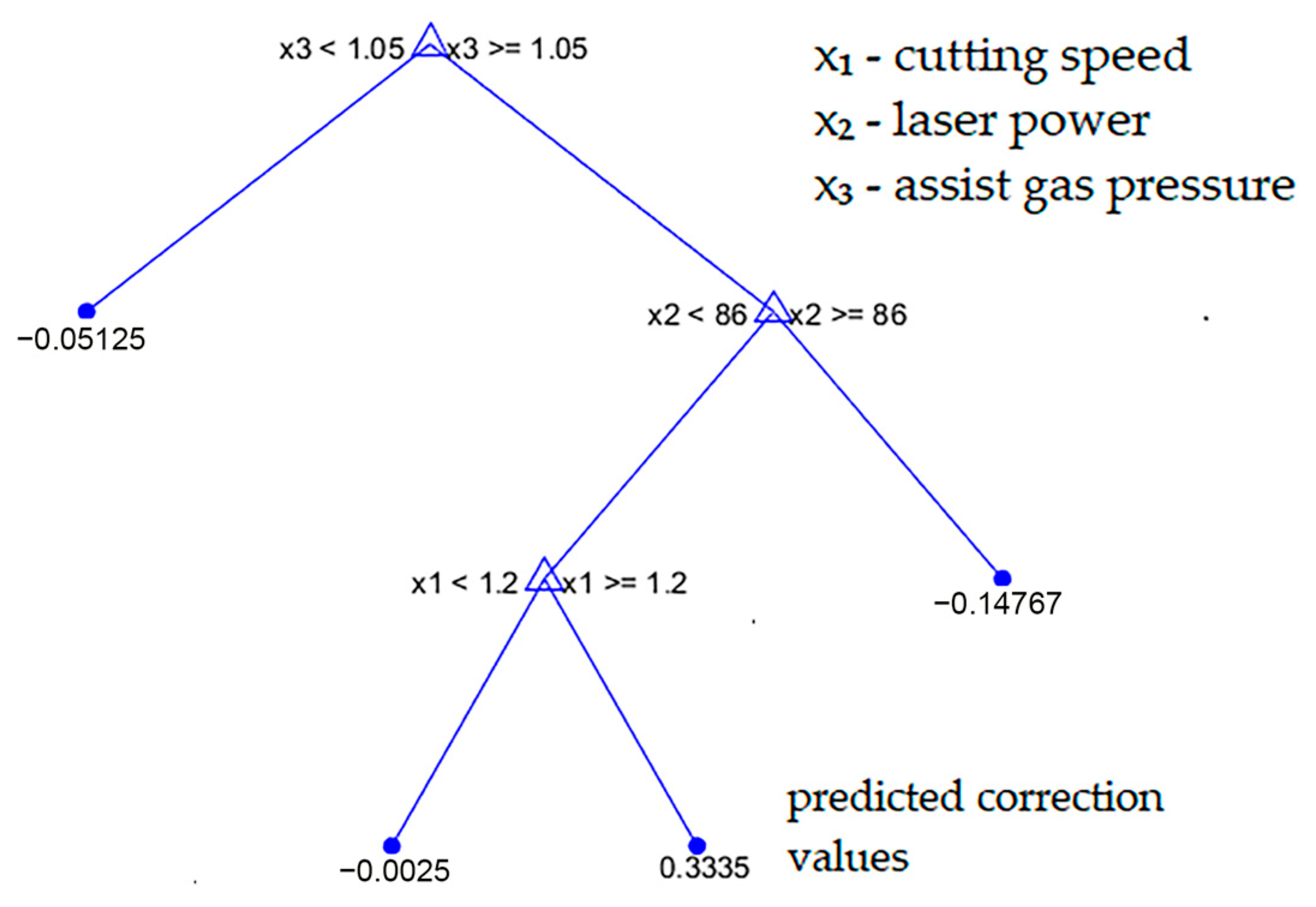
The structure of the regression tree model is shown in Figure 6. Each internal node represents a binary partition based on a threshold value of one of the input parameters cutting speed, laser power, or auxiliary gas pressure chosen to minimize the prediction error. These decision rules divide the input space into regions with similar residual behavior. The end nodes (leaves) indicate the predicted correction values that are added to the RSM output, along with the number of samples associated with each region. The overall depth and branching pattern of the tree reflect the ability of the model to isolate localized nonlinear effects within the residuals. This graphical representation provides a transparent and interpretable view of how the hybrid model adjusts the original predictions to bring them more in line with the experimental data.

The resulting hybrid model, which combines RSM predictions with machine learning-based residual correction, achieved an improved R² of 0.8889. This demonstrates that the regression tree successfully modeled the nonlinear deviations unaccounted for by the RSM model.

Figure 7 shows a comparison between the experimental surface roughness values, the predictions from the RSM model, and the corrected predictions from the hybrid model. The hybrid model matches the experimental data more closely across the entire range, especially in areas where the RSM model showed noticeable deviation.

The performance gains of the hybrid model are further quantified in Figure 8 and Figure 9, which compare the RMSE and R² values, respectively. As shown in Figure 8, the hybrid model reduced the RMSE from 0.2169 µm to 0.1717 µm, representing a 20.85% reduction in prediction error. Similarly, Figure 9 shows that the R² value increased from 0.8227 to 0.8889, corresponding to an 8.04% improvement in the explained variance.

This modeling strategy improves prediction accuracy by decomposing the problem into two levels: the RSM model captures the dominant trends, while the regression tree isolates complex nonlinear residual patterns that RSM cannot explain. By modeling only the residuals, rather than Ra directly, the tree avoids overfitting and focuses on local correction. This layered structure results in a better fit to experimental data, as reflected by the reduction in RMSE and the increase in R².

One additional advantage of using regression trees is their interpretability. Unlike black-box models, the resulting decision rules can offer insight into specific interactions among input parameters that lead to systematic under- or overestimations in the base model.

In summary, the proposed hybrid modeling approach effectively combines the transparency of statistical regression with the adaptive capabilities of machine learning. This integration results in improved prediction accuracy and enhanced generalization, even when working with a limited experimental dataset.

3.4. Validation of the Hybrid Model Using LOOCV

Leave-one-out cross-validation (LOOCV) was employed to rigorously evaluate the generalizability of the developed hybrid model. In this approach, each of the 17 data points in the dataset was iteratively excluded from the training set and used as an independent test case. The regression tree model was retrained on the remaining samples, and the residual for the excluded point was predicted. This process was repeated for all data points, ensuring an unbiased assessment of model performance while mitigating the risk of overfitting, which is critical for small datasets.

RMSE and R² in LOOCV are performance metrics that evaluate how well a model predicts and explains variance in the dependent variable during leave-one-out cross-validation. RMSE measures the average prediction error, while R-squared reflects how much variance is captured by the model. These metrics help assess generalization, especially for small datasets, but can be sensitive to outliers. Interpretation should consider model complexity and the potential for overfitting.

In this research, the LOOCV results revealed an RMSE of 0.3241 µm and an R² of 0.6039, indicating that the predicted surface roughness (Ra) deviates by approximately 0.32 µm from experimental values. By applying LOOCV, the R² obtained is considered acceptable, depending on the application area, with values ranging from approximately 0.2 to 0.9 (i.e., 20% to 90%) [24]. This variation reflects the differing levels of model performance required across various domains. This accuracy is acceptable for industrial applications, considering typical Ra values in the laser cutting range from 2 to 3 µm [25]. Although the performance declined compared to the training results (RMSE = 0.1717, R² = 0.8889), LOOCV offers a realistic estimate of generalization. These findings confirm the practical value of the proposed model and provide a solid basis for the concluding observations in the next section.

As shown in

Table 5. Comparison of the obtained model with relevant literature in terms of R².

Study (Ref)	Method	Trials	R2
Obtained model	RSM + Tree (Hybrid)	17 (Box–Benkhen)	≈0.89
Safari et al. [26]	RSM	15 (Box–Benkhen)	≈0.93
Vinoth [27]	RSM	27 (Taguchi)	≈0.93
Salem et al. [28]	RSM	32 (Taguchi)	≈0.90

, the R² value obtained for the proposed hybrid model (≈0.89) is comparable to those reported in similar studies using traditional RSM approaches. For example, Safari et al. [26] and Vinoth [27] achieved R² values of ≈0.93 using Box–Behnken and Taguchi designs, respectively, with a similar number of experimental trials. Salem et al. [28] reported an R² of ≈0.90 based on 32 experiments. Although our study involved only 17 experimental points, the predictive performance remains consistent with these references, highlighting the effectiveness of the proposed hybrid approach.

These are often constrained by practical limitations such as machine settings, control accuracy, and technological stability during processing. Despite these constraints, the hybrid model successfully captured key process relationships, demonstrating its applicability, even with a limited dataset. It is also well recognized in the statistical literature that what is considered a good R² depends heavily on the field and context. According to published sources, R² values in the range of 0.60 to 0.90 are generally regarded as acceptable to strong for engineering and manufacturing processes, particularly when using empirical models such as RSM or hybrid learning frameworks [29]. In this regard, the obtained R² of ≈0.89 supports the practical validity of the proposed model.

4. Conclusions

This study presented a hybrid modeling approach for predicting surface roughness (Ra) in laser cutting by combining response surface methodology (RSM) with machine learning-based residual correction. A quadratic RSM model was initially developed using a Box–Behnken design, with cutting speed, laser power, and auxiliary gas pressure as input parameters. Although the RSM model achieved a reasonable fit (R² = 0.8227), it showed limitations in capturing certain nonlinear relationships between the predicted and experimental values. To address this, a regression tree algorithm was applied to model the residuals of the RSM predictions, resulting in a significant improvement in accuracy. The final hybrid model demonstrated enhanced predictive performance, achieving an R² of 0.8889 and a reduced RMSE compared to the standalone RSM model.

Leave-one-out cross-validation (LOOCV) further confirmed the model’s generalization capability, yielding an RMSE of 0.3241 µm and an R² of 0.6039. Although lower than the training performance, these results validate the model’s robustness when applied to limited experimental datasets. Comparative analysis with existing approaches such as random forest (RMSE = 0.05 µm, R² = 0.91) demonstrated the competitiveness of the proposed hybrid method, particularly in balancing predictive accuracy and interpretability.

The findings underscore the benefits of integrating classical statistical techniques with machine learning for modeling complex manufacturing processes. The hybrid approach not only enhances prediction accuracy but also preserves interpretability, making it suitable for real-world applications where data availability is limited. Future research could explore the integration of alternative machine learning algorithms or extend this methodology to additional machining parameters and material types.