Featured Application
Estimation of dynamic error signal parameters for a measurement chain containing a digital signal processing algorithm.
Abstract
This paper presents a method for estimating the parameters of the dynamic error signal in a measurement chain. The method is based on knowledge of the transmittance of subsequent elements in the chain and analysis of the spectrum of the processed signal. The proposed approach allows for determining the parts of uncertainty budget of the measurement chain related with dynamic errors, considering the currently processed signal and the calculation of the expanded uncertainty associated with the dynamic error signal. The paper describes the proposed error model, the algorithm for estimating the error signal parameters, and detail measurement and simulation experiments conducted to verify the effectiveness of the proposed method.
1. Introduction
The measurement channels of modern measurement and control equipment typically include components that perform digital processing of measurement signals [1,2,3,4]. This approach enables the use of a wide range of signal processing algorithms to extract useful information [5,6,7], apply multiplicative algorithms for power and energy measurements [8,9], analysis of power grids fails and short circuits [10,11], or perform static and dynamic reproduction of processed quantities [12,13,14,15]. Although the most important operations related to signal processing are performed digitally, the physical quantity being measured is continuous in time and must first be converted into an electrical voltage. This voltage—after being processed by the analog part of the measurement chain—is then converted into digital form by an analog-to-digital (A/D) converter. This process is shown in Figure 1.
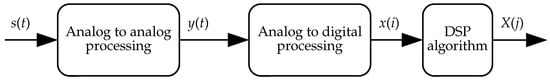
Figure 1.
Diagram of a typical implementation of a measurement chain (source [16] under the CC BY 4.0 license).
The analysis of the inaccuracy in determining the values of the output quantities of the measurement chain must therefore include a description of the analog processing, which ultimately allows for estimating the uncertainty budget of the input quantities of the A/D converter [14,17]. The next stage of the analysis is to determine the impact of the A/D conversion process on the error signals present in the output quantities of the A/D converter. The final stage is to determine the metrological properties of the digital processing algorithm (D/D). This approach has been successfully used, among others, in [14,16,18,19,20].
According to the proposal presented in the literature [14,19,21] for dividing error signals, it can be observed that the parameters of some of the above-mentioned signals are closely correlated with the waveform of the signal representing the measured physical quantity. As shown in [13,16,18,19,22,23], the dynamic error signals resulting from the imperfect transmittance of subsequent fragments of the measurement chain are closely related to the spectrum of the signal processed by the chain. Imperfect transmittance is understood as one that deviates from that assumed by the designer of the measurement chain [23]. In practice, this means that the development of the uncertainty budget of the output quantities of the measurement chain is not possible without knowing or estimating the spectrum of the input quantity processed by it. Currently, no method has been proposed in the literature that allows estimation of the parameters of the discussed error signals without knowledge of the properties of the processed signal.
To address the above-mentioned problems, this article proposes a method for estimating the parameters of the dynamic error signal of the input quantities of the digital part of the measurement chain based on the spectrum of these quantities and the error model of the analog part of the chain. The presented analysis includes various cases in which typical problems of the method are discussed and its effectiveness is demonstrated. In addition to simulation results, the article presents an example of the application of the proposed method to an exemplary measurement chain and provides the results of a measurement experiment verifying the effectiveness of the method. The article is a continuation of the considerations contained in [16,18].
The paper is divided into six sections. Section 1 discusses the current state of knowledge on the subject and presents the general concept of the work. Section 2 is devoted to the discussion of the mathematical model of the error signal, where the most important dependencies and derivations are presented. In Section 3, a proposed method for estimating the error signal parameters, discussed in Section 2, is presented. Section 4 and Section 5 are devoted to simulation and measurement verification of the proposed method, and examples of its application are indicated. The final Section 6 summarizes the most important properties of the method and presents the main conclusions from the conducted research.
2. Dynamic Error Model
Dynamic error signals are signals whose realized values change for subsequent samples of the algorithm’s input quantities within the analyzed measurement window, and the nature of these changes is deterministic. An example of such an error signal is a signal resulting from the introduction of a phase shift in the output quantities of the analog part of the measurement chain. Let us assume that a fragment of the measurement chain converts a time-varying physical quantity into a voltage signal representing it, , in accordance with the diagram in Figure 2.
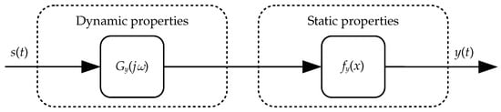
Figure 2.
Diagram of the measurement chain analog part (source [16] under the CC BY 4.0 license).
For the presented fragment of the measurement chain, a certain ideal transmittance and a processing function can be assumed, which result from the measurement task being performed. Unfortunately, the actual properties of this fragment and the quantities and describing them may differ from the ideal ones. Taking these assumptions into account, the ideal and the actual outputs of the analog part can be described by the following equations:
hence, the error signal introduced by this object can be described by Equation [13,19]:
where is the angular frequency, is the amplitude, and is the phase of the jth harmonic of signal , while the values of the introduced gain and phase shift are [24], respectively:
Assuming that the transfer function of the object is linear and time-invariant and that the processing function of the object is linear and additive, the object can be described solely by the transfer function , whose static gain equals the static sensitivity of the analyzed object [25]. Under these assumptions, and in accordance with the division proposed in [19,21], the error signal component for the harmonic constitutes the static error signal:
while the remaining harmonics contribute to the dynamic error signal:
As shown in [16,18], the most important source of the dynamic error signal in this case is the introduction of a phase shift, , by the analyzed fragment of the measurement chain, which differs from the expected value, . An additional source of the signal in question may also be the introduction by the object of a gain other than the desired one . It can be observed that the analyzed fragment of the measurement chain acts as a filter with parameters determined by its physical properties, while ideally the transmittance of this object should have the following form:
where is the sensitivity of the analyzed object. According to the adopted assumption, the ideal gain and phase characteristics are given by the following:
Assuming the measurement process is performed multiple times, the variance of the subsequent harmonics of the dynamic error signal [24] can be determined as follows:
and the expanded uncertainty can be calculated as follows:
where is the expansion factor for the sine function distribution at the assumed confidence level [17,26].
If the resulting dynamic error signal consists of many harmonics with different angular frequencies, the resultant variance of this signal is given by Equation [24]:
However, determining the expanded uncertainty for a given confidence level in this case is complex and can be achieved using methods described in [27,28,29,30,31,32,33,34]. If the error signal contains harmonics with identical angular frequencies, the resultant values of these harmonics should be determined according to the method presented in [16,24,34].
Assuming that the signal is the input quantity of the A/D converter, this converter transfers the dynamic error signal present in this signal to the output. Additionally, the converter introduces its own errors [14,35,36] to the output quantity . These error signals result from the finite resolution of the converter, imperfections of the sample-and-hold (S/H) system, inhomogeneity of the internal structure of the standard, or imperfections of the reference voltage source [35,37]. Throughout the remainder of the paper, it is assumed that the metrological properties of the S/H system are included in the error model of the analog part of the measurement chain. Hence, the value of the converter output quantity, expressed in the unit of the input quantity , is given by Equation [14]:
where is the value of a single quantum of the transducer that processes voltage in the range , where , with resolution .
Under the adopted assumptions, in the ideal case, the output quantity of the A/D converter is described by the following equation:
where is sampling period, while in the real case, this quantity is described by the following equation:
The resulting error signal at the output of the A/D converter can be described as follows:
where is the error signal due to the rounding operation in Equation (14). The dynamic error signal is then propagated to the A/D converter output according to the following equation:
where the variance of this signal is identical at the input and output of the A/D converter [16,19]:
3. Dynamic Error Parameter Estimation
According to the diagram shown in Figure 1, subsequent samples of the output quantities of the A/D converter are processed by the D/D processing algorithm used in the measurement chain. For each run of the algorithm, N subsequent samples of the signal are collected, based on which the values of the output quantities of the measurement chain are determined. To estimate the parameters of the dynamic error signal in quantity , a spectral analysis can be performed on the current vector of input samples. This analysis can be performed using the discrete Fourier transform (DFT) algorithm.
Assuming that the samples are real numbers, the output quantities of the DFT algorithm are given by Equation [3,24]:
while the amplitude , phase , and angular frequency of the output quantities are determined as follows:
for , where is the sampling rate.
By analyzing Equation (7) together with Equation (18), a single harmonic component of the dynamic error signal of quantity can be described as follows:
where the estimated realization can be approximated from the signal spectrum as follows:
In the absence of dynamic error, the ideal harmonic , without additional phase shift or attenuation, is given by the following equation:
Based on Equations (7), (11), (19), and (24), the estimated variance of the kth harmonic component of the dynamic error signal can be described as follows:
and the resultant variance of the dynamic error signal is described by the following equation:
The method presented above requires knowledge of the dependence of the resultant phase shift and gain introduced by the analog part of the measurement chain. The estimation of these parameters, based on measurement experiments and data from the catalog notes of the components used, is described in [16]. If, for the measurement chain part under discussion, the gain value for frequencies in the range closely matches the expected value (i.e., when ) and the ideal phase shift is zero (i.e., when ), then (27) simplifies to the following form:
By assuming that the difference between the actual and the ideal phase shift value is small (i.e., when ), this equation can be simplified even further:
The simplification contained in Equation (30) results from the properties of the sine and cosine functions, where for small angle measures the sine function is close to a linear function, while the cosine function assumes similar values in the indicated range of arguments. Throughout the remainder of the paper, Equation (27), without simplifications, is used. During the discussion of conclusions, selected results obtained using Equation (30) are also presented.
The analytically implemented method presented so far allows for a very accurate estimation of the dynamic error signal parameters. However, its actual implementation may encounter several problems typical when using the DFT algorithm. The most important problems in the analyzed case are aliasing, spectral leakage, and noise in the processed quantity . Aliasing can be reduced by using appropriate filters [38]. In the case of spectral leakage, an appropriate measurement window [39] can be used, while in the case of noise, it is proposed to use a method similar to the one described in [40,41], used to reduce noise in the measurement signal using the discrete wavelet transform (DWT) algorithm.
The method proposed for handling noise in the measurement signal involves rejecting harmonics with amplitude values lower than a threshold determined by the following equation [41]:
Thus, in Equation (28), the corrected amplitude values are used, defined as follows:
The application of the measurement window consists of feeding the input of the DFT algorithm, described by Equation (20), with the modified signal , described as follows:
where is the applied window function [42]. The term in the denominator normalizes the window energy to preserve the original energy of the processed signal [24]. This normalization is necessary because the estimated energy of the error signal depends on the estimated energy of the processed signal, as shown in Equation (27).
4. Simulation Verification of the Method
First, the effectiveness of the proposed method was verified by simulation. For this purpose, a series of Monte Carlo experiments [33,43] were conducted, the results of which are discussed later in the article. Each experiment involved computing the variance of the dynamic error signal 100,000 times, for a vector consisting of N samples taken at time intervals . The initial phase of the processed signal was randomly selected for each iteration. The actual variance of the dynamic error signal was determined based on Equation (13), taking into account the dependencies described by Equations (7) and (19), while the estimated variance was determined based on Equation (28). For the obtained results, the relative error in estimating the variance was determined:
along with statistical parameters of this value: the mean , standard deviation , and expanded uncertainty at a 95% confidence level [17]. The effectiveness of the proposed method for the experimental conditions was assessed based on these parameters.
During the experiments, the measurement chain converting the physical quantity into its voltage representation and then into its discrete form , which is the input for the D/D processing algorithm, was analyzed. The subsequent N values of were taken with a sampling frequency . The fragment converting to was characterized by the transfer function , assuming the following:
where is the cutoff frequency of the analog processing part (A/A). Depending on the experimental conditions, the A/D converter introduced a quantization error to , and the measured quantity was disturbed by a white noise signal with constant power spectral density and normally distributed values [44,45].
The experiments were performed using GNU Octave version 9.4.0 [46]. Equation (20) was implemented using the program’s built-in FFT function. The source code, which allows reproducing all experiments, is publicly available in the repository [47].
4.1. The Case of Spectrum Leakage
The first problem considered is the case of spectral leakage [39]. This situation occurs in the case of noncoherent sampling, i.e., when where . While the estimated energy value for the analyzed signal does not change, the output quantities of the DFT algorithm show additional harmonics with frequencies close to the actual harmonic frequency of the signal . This means that the estimated dynamic error signal contains more harmonics than actually present.
Because, according to Equation (27), the estimated variance of the kth harmonic depends on the introduced phase shift, which in turn depends on the harmonic’s frequency, this situation is unfavorable. If most of the real energy of the harmonic of leaks to a lower frequency harmonic, the variance of the dynamic error signal associated with that harmonic will be underestimated. Otherwise, due to a larger value of the phase shift parameter , this variance will be overestimated.
To verify the influence of this phenomenon on the relative error in estimating the variance of the dynamic error signal described by Equation (34), a monoharmonic signal , defined by the equation, was applied to the input of the measurement channel described in the Introduction section of this paper:
where is the angular frequency of the signal and is the initial phase of this waveform, random for each iteration of the experiment. The quantization error introduced by the A/D converter was not considered in the experiment.
The experiment was performed for the following parameter combinations: , , and for the signal frequency equal to the following:
where the multiplier . Thus, for each frequency, different cases of spectral leakage were tested, caused by failure to meet the coherent sampling condition for , as well as the case of coherent sampling where . The experiment was performed for all combinations of these parameter values. Selected results are presented in Figure 3 and summarized in Table 1. The experiment can be reproduced by running the script in the file case_1_sine.m located in the repository [47].
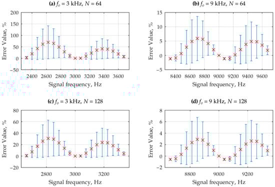

In analyzing the presented results, it can be seen that the phenomenon of spectrum leakage significantly affects the relative error in estimating the variance of the dynamic error signal and its spread. When coherent sampling conditions are maintained, the value of this error is close to zero. This phenomenon is particularly noticeable when the number of samples of the analyzed signal is low, where the frequency resolution of the DFT algorithm is limited, and for low frequencies of the signal processed by the measurement chain. As the frequency of the processed signal increases and the number of samples increases, the effect of spectrum leakage becomes less noticeable, and consequently its impact on the obtained results is minimal.
For low frequencies of the processed signal, the variance of the dynamic error signal is small, and the ratio of the frequency difference between subsequent results of the DFT algorithm is much higher than in the case of higher values of this quantity. Because this difference directly influences the estimated phase shift and consequently the estimated variance, these differences are significant in this context. However, it should be noted that the variance of the dynamic error signal is very small in this case, which, relative to the overall uncertainty budget, may have a negligible impact on the resultant variance and the expanded uncertainty of the analyzed quantity. This phenomenon is discussed in more detail later in the paper.
As mentioned in the Introduction, the phenomenon of spectral leakage can be mitigated by using an appropriate measurement window. The experiment discussed so far was repeated using the following measurement windows: “Blackman”, “Hamming”, “Bartlett”, “Hann”, and “Flat Top” [42], in accordance with Equation (33). The experiment was conducted under conditions identical to those in the previous case, with the only difference being the use of a constant input quantity vector length of . Selected experimental results are presented in Table 2 and Figure 4. The experiment can be reproduced by running the script in the file case_2_window.m, located in the repository [47].

Based on the presented results, it can be concluded that when the conditions of coherent sampling are met, the inaccuracy in estimating the variance of the dynamic error signal is greater than in the case without a measurement window. The measurement window used under coherent sampling causes the phenomenon of spectrum blurring. In the case of non-coherent sampling, the value of the discussed parameter is significantly smaller. It should be noted that, in practical measurements, achieving full sampling coherence is not possible. The use of a measurement window is therefore justified, despite the mentioned negative effects. The introduced error is small, while the inaccuracy in non-coherent sampling is significantly reduced.
Of all the measurement windows used, the “Flat Top” window showed the lowest effectiveness. The “Bartlett”, “Hann”, “Blackman”, and “Hamming” windows showed similar effectiveness. It can therefore be concluded that, for the analyzed case, dynamics are more important than window resolution. By analyzing the statistical parameters of the obtained results, it can also be observed that the “Blackman” and “Flat Top” windows show almost zero dispersion in the relative error of estimating the variance. Because the “Hamming” measurement window showed the greatest effectiveness for the analyzed case, it is used throughout the remainder of this paper.
Given the results of the previous experiment, where 95% of the relative error values in estimating the variance for were within the range %, while in the experiment using a measurement window this range narrowed to % for the “Hamming” window, it is clear that the use of a measurement window significantly improves the accuracy of the obtained results. It should be emphasized, however, that in the first experiment, the overestimated variance values concerned cases where the variance was very small compared to other more accurately estimated cases, which may be insignificant in the background of other error signals. Therefore, the advantages and disadvantages of using a measurement window should be considered in terms of computational complexity and potential impact on the accuracy of the obtained results. This topic is further discussed later in the paper.
4.2. The Case of Random Error Signals
According to the classification proposed in [16,19,48], the group of random error signals includes signals whose realization values vary within a single measurement window, and this variation is nondeterministic. The parameters of such signals can be described probabilistically by their variance and the probability density function representing the likelihood of obtaining a particular realization. An example of this type of signal is the quantization error, as defined by Equation (14). Another example is the presence of white noise in the measurement signal.
To assess the influence of random error signals on the effectiveness of the proposed method, an experiment was carried out in which the signal was applied to the input of the measurement chain in the following form:
where represents white noise with zero mean, constant power spectral density , and normally distributed realizations [44,45]. The experiment was conducted for a given signal-to-noise power ratio, defined for the experimental conditions by the following equation:
where results from the unit amplitude and zero mean of the fundamental harmonic of the signal . The quantization error introduced by the A/D converter was not considered in this experiment.
The experiment was performed using the following parameter combinations: , , , and a signal frequency defined by Equation (38), where the multiplier . Selected results are presented in Table 3 and Figure 5. The experiment can be reproduced by running the script in the file case_3_noise.m located in the repository [47].
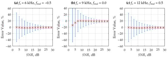
The results of the experiment indicate that using the method described by Equation (32) produces a relative error in estimating the variance of the dynamic error signal that is close to zero and reduces the variability of the estimate. It can also be observed that the method does not cause negative effects in cases where no noise is present. Although the expected value of the parameter remains close to zero regardless of the ratio of useful signal power to noise, its dispersion increases as this ratio decreases. In practice, this means that for highly noisy signals, the uncertainty of estimating the variance value becomes significantly larger. It should be noted that the discussed experiment was conducted for values much lower than those typically found in measurement chains [16,17].
4.3. Case of the Error Model Parameter Inaccuracy
Since the presented analysis method requires knowledge of the transfer function of the subsequent elements of the measurement chain, its effectiveness depends on the accuracy of the estimation of this transmittance. Assuming that and are estimated values of the actual parameters and , we can write
where is the correctly estimated value of the variance of the k-th harmonic of the dynamic error signal (in the case of knowing the actual transfer function ), while is the variance value estimated on the basis of inaccurately determined values of the parameters and .
For the discussed case the relative error in estimating the variance value of the kth harmonic of the dynamic error signal with pulsation , presented earlier in Equation (34), takes the form
so after substituting Equations (41) and () into Equation (43), one can write
For the rest of the experiments described in the paper, it is assumed that the parameters of the measurement chain error model were determined correctly, therefore holds. Analyzing the content of Equation (44), it can be noticed that the inaccuracy of the gain parameter estimation has a greater impact on the effectiveness of the proposed analysis method than the inaccuracy of the phase shift parameter estimation. Analyzing the measurement experiment described in work [16] it can be noticed, however, that in the case of the gain value, determining the dependence of this quantity on the pulsation of the signal processed by the measurement chain is much easier than in the case of determining this dependence for the phase shift.
4.4. Comprehensive Verification of the Effectiveness of the Method
The previous experiments allowed for the evaluation of the effectiveness of the proposed method in various conditions. The final measurement experiment presents a complex case in which the analyzed measurement chain processes a polyharmonic input signal given by the following equation:
where for each iteration of the experiment, the parameters of this waveform were randomly selected. The value of the constant component was ; the amplitudes of the subsequent harmonics were ; the angular frequencies were ; the phase values were ; and the variance of the white noise signal was (therefore, according to Equation (40), dB). Symbol denotes uniform distribution [44].
During the experiment, the contribution of the A/D converter to the uncertainty budget of the quantity was additionally taken into account. Therefore, for the discussed case, in accordance with (14), this quantity is described by the following equation:
where the quantity , which depends on described by Equation (45), is defined by Equations (1) and (2). The value of the quantum is .
The experiment was carried out for a variable length N of the input quantity sample vector and for a varying number K of harmonic components of the signal . During the experiment, the method used the “Hamming” window and the algorithm for reducing the impact of the noise signal on the effectiveness of the proposed method, as described by Equation (32). Due to the large variability in the parameters of the dynamic error signal, Equation (27) was used to estimate its variance, without any simplifications. Selected results from the experiment are shown in Figure 6. The experiment can be reproduced by running the script in the file case_4_mix.m located in the repository [47].
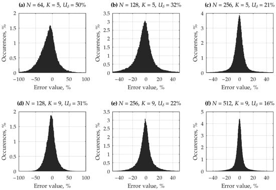
Figure 6.
Histograms of the obtained values of the realization of the relative error in the estimation of the variance of the dynamic error signal (34) for the input signal (45), depending on the adopted experiment parameters (selected cases using the “Hamming” window function, with expanded uncertainty at a 95% confidence level).
By analyzing the presented histograms, it can be observed that the expected value of the relative error in estimating the variance of the dynamic error signal is close to zero, while the spread of this value is noticeable. However, it should be noted that a significant portion of the parameter combinations of the processed signal exhibited very unfavorable conditions for the applied algorithm. These cases include the presence of several signals with very similar frequencies, which intensified the phenomenon of spectral leakage, the presence of multiple low-frequency signals, and a large share of noise compared to the useful part of the processed signal. By examining the results, it can be seen that the effectiveness of the proposed method increases as the length of the input quantity vector increases, which directly improves the frequency resolution of the DFT algorithm. However, within the context of this research, the proposed method can be considered suitable for measurement practice [17], provided it is applied using parameters that are appropriate for the characteristics of the error signal, the variance of which is being estimated. It should be further emphasized that the ultimate goal of this method is to estimate the uncertainty value, which is proportional to the square root of the variance. Therefore, the discrepancy in estimating this parameter will be considerably smaller.
Based on the results shown in Figure 6, it can be concluded that the accuracy of estimating the variance of the dynamic error signal under the experimental conditions depends mainly on the frequency domain resolution of the DFT algorithm. For the same value of N, both the spread and the expected value of the analyzed parameter do not change significantly with an increase in the number of harmonics of the processed signal.
5. Measurement Verification of the Effectiveness of the Proposed Method
The measurement verification of the effectiveness of the discussed method was performed on the measurement chain, the error model and metrological properties of which were described in [16]. A schematic diagram is shown in Figure 7. This measurement chain processes the time-varying voltage , which is first conditioned by the A/A processing system into the signal and then converted into the form by the A/D converter. The analyzed quantity is defined as follows:
where is the sampling period corresponding to the sampling frequency , and is the resultant error signal of magnitude , which consists of the following:
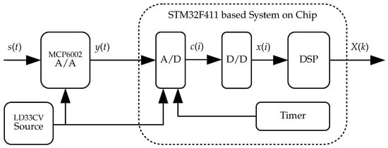
Figure 7.
Schematic diagram of the analyzed measurement chain (source: [16] under the CC BY 4.0 license).
- —resultant random error signal with constant power spectral density, zero expected value, normally distributed realization values, and variance of 0.13 ,
- —resultant dynamic error signal, whose variance values for subsequent harmonics is estimated using the proposed method.
According to the considerations in [16], the origin of the dynamic error signal for the discussed measurement chain is the imperfect dynamics of the operational amplifier operating in a non-inverting configuration, whose cutoff frequency is about 165 kHz. This component introduces a significant phase shift:
for a harmonic with angular frequency , where for the ideal measurement task, . Regarding gain values, it can be assumed that for frequencies in the range , holds.
Therefore, the information presented in [16] concerning the metrological properties of the analyzed measurement chain allows direct application of the proposed method to estimate the variance of the dynamic error signal. In this section of the paper, the proposed algorithm is applied to the quantity , which in this case is the input to the Discrete Wavelet Transform (DWT) algorithm.
For the given parameters of the signal , 30,000 sets of subsequent values of the realization of the quantity were collected, with the initial phase of the signal randomized. The proposed method for estimating the variance of the dynamic error signal was applied to the obtained samples. Then, the trajectory/realization/behavior of the error signal and its variance were estimated according to Equation (48), based on which the actual value of the variance of the dynamic error signal was estimated:
It should be noted that the variance estimated according to Equation (50) may be higher in practice than the actual variance of the dynamic error signal . This equation assumes that, apart from the errors mentioned in the Introduction, there are no other significant sources of error. This assumption may not be entirely accurate, but without knowledge of the exact error model of the entire measurement chain, determining the exact value of this parameter is not possible.
5.1. The Case of a Monoharmonic Signal
Although the application of the proposed method does not require prior knowledge of the processed signal, verifying its effectiveness must be based on certain assumptions that allow for determination of the true value of the estimated parameter. In the first experiment, a sinusoidally varying signal described by the following equation was applied to the input of the measurement chain:
where is the amplitude, is the direct current (DC) component, is the phase, and is the angular frequency of the signal. The source of the signal was the RIGOL DG1011 [49] arbitrary waveform generator, and the amplitude setpoints were verified using an additional Agilent 3458A [50] multimeter, assuming that , where is the effective value of the signal indicated by the instrument [24].
The experiment was performed for various frequencies of the waveform with amplitude and constant component . The determined relative errors in estimating the variance of the dynamic error signal for this experiment are presented in Table 4, while histograms of the realization values of this quantity for selected experiment parameters are shown in Figure 8.
Table 4.
Results * of the measurement experiment for the case of the monoharmonic signal described in Equation (51) (with expanded uncertainty at a 95% confidence level).
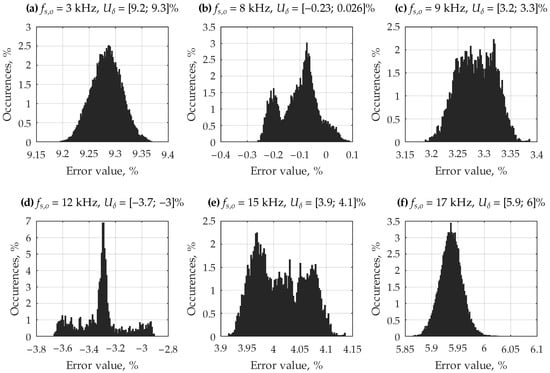
Figure 8.
Histograms of the realization values of the relative error in estimating the variance of the dynamic error signal (selected cases of monoharmonic signal, with expanded uncertainty at a 95% confidence level).
5.2. The Case of a Polyharmonic Signal
The final measurement experiment concerned the case where the input of the analyzed measurement chain was supplied with a polyharmonic input signal described by the following equation:
where is the DC component, is the amplitude, is the angular frequency, and is the phase shift of the fundamental harmonic of the signal. The source of the signal was the RIGOL DG1011 [49] arbitrary waveform generator, and the amplitude setpoints were verified using an additional Agilent 3458A [50] multimeter, assuming that , where is the effective value of the signal indicated by the instrument [24].
The experiment was performed for various frequencies of the waveform, with amplitude and constant component . The determined relative errors in estimating the variance of the dynamic error signal for this experiment are presented in Table 5, while histograms of the realization values of this quantity for selected parameters are shown in Figure 9.
Table 5.
Results * of the measurement experiment for the case of the polyharmonic signal described in Equation (51) (with expanded uncertainty at a 95% confidence level).
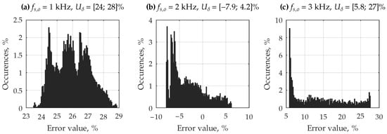
Figure 9.
Histograms of the realization values of the relative error in estimating the variance of the dynamic error signal (selected cases of polyharmonic signal, with expanded uncertainty at a 95% confidence level).
5.3. Analysis of the Obtained Measurement Results
In analyzing the results of the conducted experiments, it can be seen that the proposed method is suitable for use with a typical measurement chain built using a “system-on-chip” solution. For selected experimental conditions, the relative error in estimating the variance value exceeds ±10%, but it should be emphasized that a similar magnitude of discrepancies was observed using the analytical method in [16]. As in the cited work, the cause of the discrepancy between the obtained results is the inaccuracy in determining the parameters of the error model of the analyzed measurement chain and the presence of additional error signals, the parameters of which were not estimated accurately enough or were completely omitted, being considered insignificant.
By comparing the results of the measurement and simulation experiments, it can be seen that in the simulation case, the expected value of the estimated parameter was consistently very close to the true value. The variability of this value, and consequently the relative error dispersion, resulted from confounding factors discussed in the description of the experiments. Therefore, it can be concluded that in the measurement experiment, the non-zero expected value of the relative estimation error does not arise from the properties or specificity of the proposed method.
In the case of the applied measurement chain, the DWT algorithm was used, the implementation of which was made in the matrix form as show in [51]. The output quantities of the algorithm were determined according to the method described in the work [18], using for this purpose the function arm_mat_mult_f32 contained in the CMSIS-DSP [4] library. At a sampling frequency of 48 kHz, collecting the vector of input quantities needed to perform a single iteration of the measurement of the used algorithm took 2.67 ms, while the time needed to determine the vector of output quantities of this algorithm was 1.85 ms. The realization of Equation (20) was implemented using the arm_rfft_fast_f32 function of the CMSIS-DSP [4] library, where the time required to perform the calculations was 0.069 ms. The time required to estimate the variance value according to Equation (28) was 0.086 ms, where Equation (21) was implemented using the arm_cmplx_mag_f32 function of the CMSIS-DSP [4] library. It can therefore be seen that in the presented measurement system, the proposed method can be used in real time. The source code of the program used in the discussed measurement system can be found in [52] repository.
An alternative to using the matrix form of the algorithm can be a recursive implementation, in which the wavelet transform algorithm is treated as a pair of filters [7]. This approach was used in the [53] library, where for the case of the analyzed measurement chain, the time needed to implement the wavelet transform algorithm using the discussed method is 0.981 ms. It should be noted here that the originally proposed method presenting the wavelet transform algorithm in the matrix form is much more universal and simpler to implement, which is why it is more user-friendly for the measurement chain designer than the solution proposed in [53]. Regardless of the method of implementing the algorithm, it can be noticed that for the analyzed measurement chain, the time needed to perform calculations is much shorter than the acquisition time of a single vector of input quantities of this algorithm, hence the system can operate in continuous mode.
6. Conclusions
The presented experiments show that the proposed method is effective and suitable for the assigned task. The expected relative error in estimating the variance of the dynamic error signal is close to zero in all analyzed scenarios, where both the measurement window and the correction method for the DFT algorithm output were used. The variability of this effectiveness indicator depended directly on the application conditions mainly on the noise level in the processed measurement signal.
Using a measurement window during the application of the proposed method is necessary to mitigate the effects of spectral leakage. The measurement window used should have good dynamic characteristics, with resolution being a secondary consideration in this case. Because the use of the “Bartlett” measurement window during the experiments produced results very similar to those of the “Hamming” window, it is recommended for cases where lower computational complexity is important. Using a low-dynamic measurement window increases the expected value of the relative error in estimating the variance of the dynamic error signal.
Correcting the amplitude value of the DFT algorithm coefficients before applying the method is necessary when random error signals are present in the processed measurement signal. This correction algorithm allows obtaining an expected value of the estimated quantity close to zero, while its variability is directly proportional to the ratio of noise power to useful signal power. The operation of the proposed correction algorithm does not affect the effectiveness of the proposed method when these error signals are absent.
The experiments showed that the simplifications proposed in Equation (30) do not significantly affect the effectiveness of the proposed method. This is an important property because the form of Equation (27) is much more complex. This property holds both when spectral leakage occurs and when noise is present in the measurement signal.
Therefore, the presented method makes it possible to estimate the parameters of the dynamic error signal associated with the input quantities of digital signal processing algorithms, enabling the development of an uncertainty budget for the output quantities without prior knowledge of the spectrum or nature of the processed signal. Applications of the proposed method may include cases where wavelet transformation algorithms [5,6,7,10,11,16,18] are used in the measurement chain or multiplicative algorithms used during power and energy measurement [8,9].
The use of the proposed method enables the development of the uncertainty budget of the output quantities of the measurement chain, using various types of data processing algorithms. This operation is extremely important when, based on the analysis of the values of these quantities, a decision related to the task being performed is made, for example, on the activation of protections related to the detection of a short circuit or a fault in the transmission network [10,11]. This work, together with the works [16,18,23,51], is a comprehensive guide to metrological analysis in the described cases. It should be noted here that this analysis is most often omitted, mainly due to the high degree of complexity or the lack of appropriate mathematical models.
Another approach to solving the problem presented in this paper may be to use the Prony’s method [54] to estimate the spectrum of the signal processed by the measurement chain. This method is resistant to the phenomenon of spectrum leakage and can be used when the processed signal contains noise. It should be noted, however, that the discussed method requires an appropriate selection of the model order and is also characterized by greater computational complexity. A significant disadvantage of the Prony’s method is also the need to solve a system of equations, but in the case of the CMSIS-DSP [4] library available for the ARM platform, there is no ready implementation of the algorithm enabling this operation.
Author Contributions
Data curation, Ł.D.; Formal analysis, M.K. and J.R.; Funding acquisition, M.K.; Investigation, Ł.D.; Methodology, M.K. and Ł.D.; Project administration, M.K.; Resources, Ł.D.; Software, Ł.D.; Supervision, J.R.; Validation, M.K. and J.R.; Writing—original draft, Ł.D.; Writing—review and editing, M.K. and J.R. All authors have read and agreed to the published version of the manuscript.
Funding
This research was partially funded by Rector of Silesian University of Technology grant number 05/020/RGJ25/0094.
Institutional Review Board Statement
Not applicable.
Informed Consent Statement
Not applicable.
Data Availability Statement
All data related to the simulation experiments supporting the conclusions of this article can be replicated using examples provided on GitHub [47]. The raw data obtained from measurement experiments will be made available by the authors upon request.
Conflicts of Interest
The authors declare no conflicts of interest.
Abbreviations
The following abbreviations are used in this manuscript:
| A/A | Analog-to-analog |
| A/D | Analog-to-digital converter |
| DC | Direct current |
| D/D | Digital-to-digital |
| DFT | Discrete Fourier transform |
| DWT | Discrete wavelet transform |
| S/H | Sample-and-hold |
References
- Saleh, R.; Wilton, S.; Mirabbasi, S.; Hu, A.; Greenstreet, M.; Lemieux, G.; Pande, P.P.; Grecu, C.; Ivanov, A. System-on-chip. Proc. IEEE 2006, 94, 1050–1069. [Google Scholar] [CrossRef]
- Reay, D.S. Digital Signal Processing Using the ARM Cortex M4; John Wiley & Sons: Hoboken, NJ, USA, 2015. [Google Scholar]
- Oppenheim, A.V.; Schafer, R.W. Discrete-Time Signal Processing, 3rd ed.; Pearson: London, UK, 2009. [Google Scholar]
- ARM Limited. CMSIS-DSP—Embedded Compute Library for Cortex-M and Cortex-A. 2024. Available online: https://arm-software.github.io/CMSIS-DSP (accessed on 20 June 2025).
- Mallat, S. A Wavelet Tour of Signal Processing, 3rd ed.; Academic Press: Cambridge, MA, USA, 2008. [Google Scholar]
- Addison, P.S. The Illustrated Wavelet Transform Handbook: Introductory Theory and Applications in Science, Engineering, Medicine and Finance, 2nd ed.; CRC Press: Boca Raton, FL, USA, 2017. [Google Scholar]
- Akujuobi, C.M. Wavelets and Wavelet Transform Systems and Their Applications; Springer: Berlin/Heidelberg, Germany, 2022. [Google Scholar]
- Alegria, F. Using digital methods in active power measurement. Acta IMEKO 2023, 12, 1–8. [Google Scholar] [CrossRef]
- Pandey, S. Analog Multiplier Based Single Phase Power Measurement. J. Electr. Electron. Syst. 2016, 5, 1–4. [Google Scholar] [CrossRef]
- Liu, Z.; Zhao, Z.; Huang, G.; Wang, F.; Wang, P.; Liang, J. Power Grid Faults Diagnosis Based on Improved Synchrosqueezing Wavelet Transform and ConvNeXt-v2 Network. Electronics 2025, 14, 388. [Google Scholar] [CrossRef]
- Altaie, A.S.; Abderrahim, M.; Alkhazraji, A.A. Transmission Line Fault Classification Based on the Combination of Scaled Wavelet Scalograms and CNNs Using a One-Side Sensor for Data Collection. Sensors 2024, 24, 2124. [Google Scholar] [CrossRef]
- Agarwal, S.; Sharma, S.; Rahman, M.H.; Vranckx, S.; Maiheu, B.; Blyth, L.; Janssen, S.; Gargava, P.; Shukla, V.K.; Batra, S.; et al. Air quality forecasting using artificial neural networks with real time dynamic error correction in highly polluted regions. Sci. Total Environ. 2020, 735, 139454. [Google Scholar] [CrossRef]
- Volosnikov, A.S. Measurement System Based on Nonrecursive Filters with the Optimal Correction of the Dynamic Measurement Error. Meas. Tech. 2023, 65, 720–728. [Google Scholar] [CrossRef]
- Jakubiec, J.; Roj, J. Error Analysis of Analytical and Neural Real-Time Reconstruction of Analog Signals; Wydawnictwo Politechniki Śląskiej: Gliwice, Poland, 2024. [Google Scholar] [CrossRef]
- Roj, J. Estimation of the artificial neural network uncertainty used for measurand reconstruction in a sampling transducer. IET Sci. Meas. Technol. 2014, 8, 23–29. [Google Scholar] [CrossRef]
- Kampik, M.; Roj, J.; Dróżdż, L. Error Model of a Measurement Chain Containing the Discrete Wavelet Transform Algorithm. Appl. Sci. 2024, 14, 3461. [Google Scholar] [CrossRef]
- Joint Committee for Guides in Metrology. Evaluation of Measurement Data—Guide to the Expression of Uncertainty in Measurement; JCGM: Sèvres, France, 2008; Available online: https://www.bipm.org/documents/20126/2071204/JCGM_100_2008_E.pdf (accessed on 20 June 2025).
- Kampik, M.; Roj, J.; Dróżdż, L. Estimation of the resultant expanded uncertainty of the output quantities of the measurement chain using the discrete wavelet transform algorithm. Appl. Sci. 2024, 14, 3691. [Google Scholar] [CrossRef]
- Jakubiec, J.; Konopka, K. The error based model of a single measurement result in uncertainty calculation of the mean value of series. Probl. Prog. Metrol. 2015, 20, 75–78. [Google Scholar]
- Jakubiec, J. Reducing interval arithmetic in dynamic error evaluation. In Proceedings of the 5th International Workshop on ADC Modelling and Testing, XVI IMEKO World Congress, Wien, Austria, 26–28 September 2000; pp. 100–105. [Google Scholar]
- Ruhm, K.H. Deterministic, Nondeterministic Signals; Institute for Dynamic Systems and Control: Zurich, Switzerland, 2008. [Google Scholar]
- Shi, S.; Yang, L.; Lin, J.; Long, C.; Deng, R.; Zhang, Z.; Zhu, J. Dynamic Measurement Error Modeling and Analysis in a Photoelectric Scanning Measurement Network. Appl. Sci. 2019, 9, 62. [Google Scholar] [CrossRef]
- Dróżdż, L.; Roj, J. Origin and properties of own error signals of the discrete wavelet transform algorithms. Int. J. Electron. Telecommun. 2024, 70, 643–648. [Google Scholar] [CrossRef]
- Oppenheim, A.V.; Willsky, A.S.; Nawab, S.H. Signals & Systems, 2nd ed.; Pearson: London, UK, 2013. [Google Scholar]
- Proakis, J.G.; Manolakis, D.G. Digital Signal Processing: Principles, Algorithms and Applications, 5th ed.; Pearson: London, UK, 2021. [Google Scholar]
- Horalek, V. Analysis of basic probability distributions, their properties and use in determining type B evaluation of measurement uncertainties. Measurement 2013, 46, 16–23. [Google Scholar] [CrossRef]
- Kampik, M.; Roj, J.; Dróżdż, L. A Method for Estimating the Resultant Expanded Uncertainty Value Based on Interval Arithmetic. Appl. Sci. 2024, 14, 7334. [Google Scholar] [CrossRef]
- Koliander, G.; El-Laham, Y.; Djurić, P.M.; Hlawatsch, F. Fusion of probability density functions. Proc. IEEE 2022, 110, 404–453. [Google Scholar] [CrossRef]
- Zhang, Z.; Wang, J.; Jiang, C.; Huang, Z.L. A new uncertainty propagation method considering multimodal probability density functions. Struct. Multidiscip. Optim. 2019, 60, 1983–1999. [Google Scholar] [CrossRef]
- Dieck, R.H. Measurement Uncertainty: Methods and Applications; ISA: Dubai, United Arab Emirates, 2017. [Google Scholar]
- Yang, L.; Guo, Y. Combining pre-and post-model information in the uncertainty quantification of non-deterministic models using an extended Bayesian melding approach. Inf. Sci. 2019, 502, 146–163. [Google Scholar] [CrossRef]
- Urbanski, M.K.; Wąsowski, J. Fuzzy approach to the theory of measurement inexactness. Measurement 2003, 34, 67–74. [Google Scholar] [CrossRef]
- Joint Committee for Guides in Metrology. Evaluation of Measurement Data—Propagation of Distributions Using a Monte Carlo Method; JCGM: Sèvres, France, 2008; Available online: https://www.bipm.org/documents/20126/2071204/JCGM_101_2008_E.pdf (accessed on 20 June 2025).
- Dróżdż, L. Reductive Interval Arithmetic Method Application Example on GitHub, 2024. Available online: https://github.com/Kuszki/Octave-Uncertainty-RIA-Example (accessed on 20 June 2025).
- STMicroelectronics. Application note AN1636; STMicroelectronics: Geneva, Switzerland, 2003. [Google Scholar]
- Baker, B.C. Optimize Your SAR ADC Design; Texas Instruments Inc.: Dallas, TX, USA, 2019. [Google Scholar]
- Arpaia, P.; Baccigalupi, C.; Martino, M. Metrological characterization of high-performance delta-sigma ADCs. In Proceedings of the 2018 IEEE International Instrumentation and Measurement Technology Conference (I2MTC), Houston, TX, USA, 14–17 May 2018; pp. 1–6. [Google Scholar] [CrossRef]
- Hajek, K.; Kohl, Z. Multiple Aliasing of Windowed Real-Valued Signal as a Cause of Accuracy Limitation of DFT Methods. IEEE Access 2025, 13, 6515–6526. [Google Scholar] [CrossRef]
- Qian, W.; Xiao, Y.; Yong, R. Spectrum leakage suppression for multi-frequency signal based on DFT. In Proceedings of the 2017 13th IEEE International Conference on Electronic Measurement & Instruments (ICEMI), Yangzhou, China, 20–23 October 2017; pp. 394–399. [Google Scholar] [CrossRef]
- Vimala, C.; Priya, P.A. Noise reduction based on Double Density Discrete Wavelet Transform. In Proceedings of the 2014 International Conference on Smart Structures and Systems (ICSSS), Chennai, India, 9 October 2014; pp. 15–18. [Google Scholar] [CrossRef]
- Halidou, A.; Mohamadou, Y.; Ari, A.A.A.; Zacko, E.J.G. Review of wavelet denoising algorithms. Multimed. Tools Appl. 2023, 82, 41539–41569. [Google Scholar] [CrossRef]
- Prabhu, K.M.M. Window Functions and Their Applications in Signal Processing; Taylor & Francis: Boca Raton, FL, USA, 2014. [Google Scholar] [CrossRef]
- Janssen, H. Monte-Carlo based uncertainty analysis: Sampling efficiency and sampling convergence. Reliab. Eng. Syst. Saf. 2013, 109, 123–132. [Google Scholar] [CrossRef]
- Grimmett, G.; Stirzaker, D. Probability and Random Processes, 4th ed.; Oxford University Press: Oxford, UK, 2020. [Google Scholar]
- Kuo, H.H. White Noise Distribution Theory; CRC Press: Boca Raton, FL, USA, 2018. [Google Scholar] [CrossRef]
- Eaton, J.W. GNU Octave Official Website. 2024. Available online: https://octave.org/ (accessed on 20 June 2025).
- Dróżdż, L. Dynamic Error Parameters Estimation Example on GitHub, 2025. Available online: https://github.com/Kuszki/Octave-Uncertainty-DEPE-Example (accessed on 20 June 2025).
- Topór-Kaminski, T.; Jakubiec, J. Uncertainty modelling method of data series processing algorithms. In Proceedings of the IMEKO TC-4 Symposium on Development in Digital Measuring Instrumentation and 3rd Workshop on ADC Modelling and Testing, Naples, Italy, 17–18 September 1998; Volume 2, pp. 631–636. [Google Scholar]
- RIGOL Technologies Inc. User’s Guide DG1-070518. 2007. Available online: https://supportjp.rigol.com/Public/Uploads/uploadfile/files/20210729/DSB01100-1110.pdf (accessed on 20 June 2025).
- Agilent Technologies Inc. Agilent 3458A Multimeter. 2011. Available online: https://dfzk-www.oss-cn-beijing.aliyuncs.com/www-PRD/resources/files/Ag_3458A_UserGuide_en.pdf (accessed on 20 June 2025).
- Roj, J.; Dróżdż, L. Propagation of Random Errors by the Discrete Wavelet Transform Algorithm. Electronics 2021, 10, 764. [Google Scholar] [CrossRef]
- Dróżdż, L. STM32F411 Sampler Using FWT and DSP Package Project on GitHub. 2025. Available online: https://github.com/Kuszki/F411-FWT-Sampler (accessed on 20 June 2025).
- Montalivet, E. A C Implementation of the One Dimensional Discrete Wavelet Transform (DWT) Based on CMSIS Library. 2025. Available online: https://github.com/etiennedemontalivet/arm-dwt-c-library (accessed on 20 June 2025).
- Zygarlicki, J.; Zygarlicka, M.; Mroczka, J.; Latawiec, K.J. A reduced Prony’s method in power-quality analysis—Parameters selection. IEEE Trans. Power Deliv. 2010, 25, 979–986. [Google Scholar] [CrossRef]
Disclaimer/Publisher’s Note: The statements, opinions and data contained in all publications are solely those of the individual author(s) and contributor(s) and not of MDPI and/or the editor(s). MDPI and/or the editor(s) disclaim responsibility for any injury to people or property resulting from any ideas, methods, instructions or products referred to in the content. |
© 2025 by the authors. Licensee MDPI, Basel, Switzerland. This article is an open access article distributed under the terms and conditions of the Creative Commons Attribution (CC BY) license (https://creativecommons.org/licenses/by/4.0/).