Article

Mode Shape Extraction with Denoising Techniques Using Residual Responses of Contact Points of Moving Vehicles on a Beam Bridge

School of Civil Engineering and Architecture, Hainan University, Haikou 570228, China
*
Author to whom correspondence should be addressed.
Appl. Sci. 2025, 15(13), 7059; https://doi.org/10.3390/app15137059
Submission received: 13 May 2025 / Revised: 15 June 2025 / Accepted: 20 June 2025 / Published: 23 June 2025
(This article belongs to the Special Issue Advances in Architectural Acoustics and Vibration)

Abstract

This work introduces a novel approach to extract beam bridge mode shapes using the residual response between consecutive contact points of vehicles passing through a bridge. A comprehensive investigation is conducted on several critical parameters, including window size, vehicle velocity, road roughness, and beam damping property, as well as the influence of traffic flow. To enhance the mode shape extraction performance using the approximate expression of the contact points’ displacements under noisy disturbance, two new signal denoising methods, CEEMDAN-NSPCA and CEEMDAN-IWT, are proposed based on complete ensemble empirical mode decomposition (CEEMDAN). CEEMDAN-NSPCA integrates CEEMDAN with principal component analysis and a coefficient-based filtering strategy. While CEEMDAN-IWT utilizes an improved wavelet thresholding technique with adaptive threshold selection. The numerical simulations demonstrate that both methods could effectively attenuate high-frequency noise with small amplitudes and retain low-frequency components. Among them, CEEMDAN-IWT exhibits superior denoising performance and greater stability, making it particularly suitable for robust modal identification in noisy environments.

1. Introduction

The extraction of modal parameters is essential for the dynamic analysis, damage detection, and model updating of bridges. Recently, significant advancements have been made in the experimental modal analysis of bridges, particularly in utilizing moving vehicles as an excitation source for damage detection [1,2,3]. Compared to natural frequencies, mode shapes are more sensitive to local variations along the bridge caused by degradation or damage [2,4]. To improve the accuracy of bridge mode identification and effectively capture modal variations induced by structural deterioration, advanced signal processing techniques have been increasingly employed. Specifically, empirical mode decomposition (EMD) [5,6,7] and variational mode decomposition (VMD) [8] have been employed to extract intrinsic mode functions (IMFs), providing a robust and effective framework for identifying modal changes associated with bridge damage [9,10].
Compared with the widely used impulse load and steady-state load, a vehicle moving along the bridge is a cost-effective and efficient mean to excite the full bridge span in a single trip. Bridge responses can be measured directly via sensors installed on the bridge or indirectly through vehicle-mounted sensors. While direct measurements on the bridge can provide accurate data, they require extensive and costly on-site instrumentation tailored to each bridge. Alternatively, the moving vehicle serves as both an excitation source and a data collector. However, vehicle-mounted measurements primarily reflect the coupled vehicle–bridge dynamics, encompassing the bridge responses, the surface roughness, and the interaction between the vehicle and the bridge.
A variety of novel methods has been continuously developed to distinguish the bridge response from the vehicle-induced signals. Eshkevari et al. [11] proposed a new second-order blind identification method by combining the vehicle transfer function and ensemble empirical mode decomposition (EEMD) to extract the vibrations caused by surface roughness and identify bridge modes. Oshima et al. [12] tried to eliminate the interaction between the vehicle axle and the bridge surface by measuring their relative motions. Additional strategies enhance the response of the bridge by applying artificial forces [11,13] and heavy trucks [14] and employing subtraction between two consecutive vehicle responses to facilitate mode shape identification [15,16].
The contact point between a vehicle and a bridge has emerged as a critical location for damage detection [17,18] and mode recognition [13,19]. Although it is physically associated with the vehicle, the contact point’s motion could reflect the bridge’s dynamic response at time-varying positions along its length as the vehicle moves. Additionally, serving as the transmission between the vehicle and the bridge, the contact point allows for the more efficient extraction of bridge dynamics by suppressing vehicle-induced interference. Instead of one single contact point, the residual response between consecutive vehicular contact points is adopted to remove road roughness. Xu et al. [20] investigated the dynamic response relationship between the front and rear contact points of a dual-axle scanning vehicle. Furthermore, a recursive formula was developed to mitigate damping distortion. Xu et al. [21] recognized a bridge beam mode based on the contact response of dual-axle test vehicles in wavelet transforms. In addition, in a moving reference-based manner, the local short-time Fourier transform (STFT) amplitudes of these residual accelerations along the frequency ridges [13] benefit mode recognition.
However, the previous studies have demonstrated [13,22] that the majority of the energy in both the vehicle and the bridge responses is concentrated in the lower frequency range around the bridge’s fundamental natural frequency under moving loads. Consequently, the dynamical characteristic of this interaction system is not sufficiently excited at the higher frequency range. When noise is inevitably introduced during the data collection step, the higher-order mode become increasingly sensitive to noise and may seem unreliable. Therefore, an appropriate denoising method is crucial for the extraction of the accurate bridge modes, especially for those in the higher frequency range.
The commonly adopted signal denoising processing technologies include feature extraction [23], empirical mode decomposition (EMD) and its variants [24,25,26,27], the wavelet threshold [28], and a moving average filter [29]. However, these methods could not guarantee signal integrity. For instance, EMD may suffer from mode aliasing [24]. Peng et al. [25] proposed a denoising method based on ensemble empirical mode decomposition (EEMD) with multi-scale principal component analysis, which improved signal decomposition but still struggled with wavelet-based limitations. Liu et al. [26] improved EEMD to enhance the stability and reliability of EMD, although reconstruction errors remained significant. Torres [27] proposed complete ensemble empirical mode decomposition (CEEMDAN), which mitigates mode aliasing by applying EMD to white-noise-augmented signals and averaging the results. Luo [29] introduced a moving average method that was effective in suppressing periodic interference, making it particularly suitable for high-frequency oscillations. Wang et al. [28] numerically compared the denoising performances of different wavelet thresholds. Zhao et al. [30] combined CEEMDAN with threshold screening singular value decomposition (SVD) to improve the signal-to-noise ratio and preserve fault features in vibration signals. Zhang et al. [31] integrated CEEMDAN and principal component analysis (PCA) to reduce high-frequency noise while retaining low-frequency information and minimizing mode aliasing. However, this technology relied on single-noise involved assumptions and involved lossy PCA-based compression, which may lead to information loss due to repeated decomposition.
To balance noise suppression and signal detail retention in the denoising process, a novel method named CEEMDAN-NSPCA is presented in this work. Unlike conventional methods that standardize input signals, it may potentially amplify noise, and this method avoids standardizing the signal and instead focuses on preserving low-frequency components while denoising high-frequency content. The process begins by decomposing the noisy signal using CEEMDAN to obtain intrinsic mode functions (IMFs). High-frequency IMFs are then selectively identified and subjected to dimensionality reduction using PCA, without normalization. Finally, the denoised high-frequency components are combined with the unaltered low-frequency IMFs to reconstruct a denoised signal.
In addition, the wavelet threshold is another option to improve CEEMDAN [32]. The IMF components obtained from CEEMDAN are selected by the correlation coefficient criterion and then filtered by the wavelet threshold algorithm. However, the direct removal of certain IMF components risks discarding valuable signal information alongside noise. To address these limitations, this study proposes an enhanced denoising method called CEEMDAN-IWT, which integrates CEEMDAN with an improved wavelet threshold (IWT) technique [33]. Initially, the CEEMDAN method decomposes the signal into multiple IMFs. The high-frequency IMFs are then subjected to wavelet decomposition, then filtered by the wavelet coefficients using an improved wavelet threshold. The filtered IMFs are subsequently reconstructed via wavelet inverse transform. Finally, the denoised signal is obtained by combining the reconstructed high-frequency IMFs with the original low-frequency IMFs, achieving effective noise reduction while preserving critical signal features.
Excluding the introduction, there are three sections including methodology, simulation examples, and conclusions in this work. In the methodology part, the approximate expression of the residual response between two contact points as well as denoising methods of CEEMDAN-NSPCA and CEEMDAN-IWT is expressed in detail. Then, a two-degree-of-freedom (DOF) tractor and three one-DOF tractors are simulated to travel along a 25 m simply supported beam bridge under different scenarios. The effects from STFT window size, vehicle speed, bridge surface roughness, and noise are examined. In addition, the influence of the bridge damping property is thoroughly investigated with and without traffic flow. The performance of the two proposed denoising methods is evaluated against two baseline methods, CEEMDAN-PCA and IWT, and summarized in the conclusion part.

2. Methodology

2.1. Dynamics Under Moving Vehicles

Figure 1a shows a fleet of three 1-DOF vehicles (M1, M2, and M3) that are supported by springs (k1, k2, and k3) and dashpots (c1, c2, and c3), and they move on a simply supported beam bridge at a constant velocity (Ve) with an equal space (d) between them. In Figure 1b, a beam with mass m, flexural rigidity EI, and damping c is connected to the regular rigid road at the ends without gaps. The 2-DOF vehicle with wheelbase Lc is supported by springs (kF and kR) and dashpots (cF and cR) from the beam and the regular road with rough profile ur.
Without the consideration of the damping properties of these three vehicles and the beam, the beam motion equation could be written as follows [34,35]:
m u ¨ ( x , t ) + E I u ( x , t ) = i = 1 3 [ k i ( u i u r V e ( t t i 1 ) u ( V e ( t t i 1 ) , t ) ) m i g ] δ ( x V e ( t t i 1 ) ) Γ i ( t )
where Γi(t) is defined below by the Heaviside step function He(t) to indicate the status of each vehicle on this bridge. The over-dot and the prime denote the derivative with time and space, respectively. δ is the delta function.
Γ i ( t ) = H e ( t t i 1 ) H e ( t t i 2 ) , t ( i + 1 ) , 1 = t i , 1 + Δ t , Δ t = d V e
where ti1 and ti2 are time instants when the vehicle enters and leaves the bridge.
The response of this beam could be expressed by the mode superposition method.
u ( x , t ) = j = 1 V j ( t ) ϕ j ( x )
The mode shape ϕj, the undamped natural frequency ωj of the simply supported beam mode j, and the vehicle’s natural frequency ωv,i are given below.
ϕ j ( x ) = sin ( j π x L ) , ω j = ( j π ) 2 E I m L 4 , ω v , i = k i m i
Substituting Equation (2) into Equation (1), multiplying by ϕn, and then integrating from 0 to L yields the following:
v ¨ n ( t ) + ω n 2 v n ( t ) i = 1 3 2 ω v , i 2 m i m L [ u i u ( V e ( t t i 1 ) , t ) ] ϕ n ( V e ( t t i 1 ) ) Γ i ( t ) = i = 1 3 [ 2 ω v , i 2 m i m L u r ( V e ( t t i 1 ) + 2 m i m L g ] ϕ n ( V e ( t t i 1 ) ) Δ i ( t )
A previous work [36] provided an analytical solution form for this interaction between the vehicle and the beam, and an approximate solution form is given here to demonstrate the contact point’s response to each vehicle. With the consideration of the small mass ratio (mi/mL) between the vehicle and the beam, the third term in the left side of Equation (5) could be discarded [13]. Similarly, compared to the gravity term, the roughness terms ω v , i 2 u r ( V e ( t t i 1 ) ) are very small and could also be discarded. Then Equation (5) could be simplified into an approximate form.
v ¨ n ( t ) + ω n 2 v n ( t ) = i = 1 3 2 m i m L g ϕ n ( V e ( t t i 1 ) ) Δ i ( t ) = i = 1 3 2 m i m L g sin ( n π V e ( t t i 1 ) L ) Γ i ( t )
With zero initial conditions, its solution could be determined, as shown below [13].
v n ( t ) = 1 1 q n 2 i = 1 3 2 L 3 m i g E I n 4 π 4 [ sin ( n π V e ( t t i 1 ) L ) q n sin ( ω n ( t t i 1 ) ) ] Γ i ( t ) , q n = n π V e L ω n
Meanwhile, the beam surface roughness ur should be added to the response of the contact point with the time-varied beam location x k = V e ( t t k 1 ) of each vehicle (k = 1, 2, 3).
u c , k ( t ) = j = 1 1 1 q j 2 i = 1 3 L 3 m i g E I n 4 π 4 [ cos ( j π V e ( t k 1 t i 1 ) L ) cos ( 2 j π V e t L + θ k , i ) q j [ cos ( ( ω j j π V e L ) t + θ k , i , ω j ) cos ( ( ω j t + j π V e L ) t + θ k , i , + ω j ) ] Γ i ( t ) + u r ( V e ( t t k 1 ) ) = R k ( t ) + u r ( V e ( t t k 1 ) ) θ k , i V e = j π V e ( t i 1 + t k 1 ) L , θ k , i , ω j = j π V e t k 1 L ω j t i 1 , θ k , i , + ω j = ( j π V e t k 1 L + ω j t i 1 )
There are three main frequency response components for one beam mode (j): the driving frequency (2jπVe/L) and the two frequencies (ωj jπVe/L and ωj + jπVe/L) centered at the beam natural frequency (ωj) and shifted by the half driving frequencies (jπVe/L). Due to the absence of vehicle frequency components, the response of the contact point could be a better measurement than the responses of the vehicle body [10]. Normally, the moving velocity (Ve) can be kept low to guarantee that the half driving frequencies (jπVe/L) are much smaller than the beam frequency (ωi). Then the shift in the half driving frequencies (jπVe/L) could be reduced efficiently. On the other hand, for ratio qn in Equation (7), this ratio decreases as the velocity decreases. Then the contact point’s response will be dominated by the component of the driving frequencies that are close to the static load case.
The roughness term (ur) on the right side of Equation (8) could be removed by subtracting two consecutive contact points such as uc,1 and uc,2 at their durations on the beam.
Δ u 1 , 2 ( t ) = u c , 1 ( t ) u c , 2 ( t + Δ t ) = R 1 ( t ) + u r ( V e ( t t 11 ) ) R 2 ( t + Δ t ) + u r ( V e ( t + Δ t t 11 Δ t ) ) = R 1 ( t ) R 2 ( t + Δ t )
This residual response form could reveal that the beam vibrates directly at these beam natural frequencies. The terms about the two frequencies (ωi − jπVe/L and ωi + jπVe/L) are denoted below.
B j k , i ( t ) = [ cos ( ω j t j π V e t L + j π V e t k 1 L ω j t i 1 ) cos ( ω j t + j π V e t L j π V e t k 1 L ω j t i 1 ) ]
From the residual expression of Equation (9), the subtraction Δu12(t) contains the term B j 1 , i ( t ) B j 2 , i ( t + Δ t ) , which could be rewritten after some operations.
B j 1 , i ( t ) B j 2 , i ( t + Δ t ) = 2 ( sin ( ω j t ω j t i 1 ) + sin ( ω j t ω j t i 1 + ω j Δ t ) ) sin ( j π V e t L j π V e t 11 L )
Then the ratio between the subtraction terms of Δu12(t) and Δu23(t) becomes as follows.
B j 1 , i ( t ) B j 2 , i ( t + Δ t ) B j 2 , i ( t ) B j 3 , i ( t + Δ t ) = sin ( j π V e ( t t 11 ) L ) sin ( j π V e ( t t 21 ) L ) = sin ( j π V e ( t t 11 ) L ) sin ( j π V e ( t t 11 Δ t ) L )
Considering Equation (4), both the numerator and the denominator in Equation (12) present the jth beam mode shape, but with a lag of VeΔt as the distance between the contact points. Therefore, the mode shapes could be estimated from the time-varying ratio of two residual responses from the three consecutive contact points (uc,1, uc,2, and uc,3) at the bridge’s natural frequencies.

2.2. Short-Time Fourier Transform

While the fast Fourier transform (FFT) serves as a powerful and widely utilized tool for transforming signals from the time domain to the frequency domain, it exhibits inherent limitations when applied to non-stationary signals. In contrast, the short-time Fourier transform (STFT) could provide greater flexibility and effectiveness in analyzing such signals by offering time–frequency localization, capturing dynamic characteristics, enabling multi-resolution analysis, and fulfilling practical application requirements.
Through the window function w(t), the traditional Fourier transform is extended to the short-time Fourier transform (STFT) [37], which could provide the localized frequency components of the signal s(t).
S t ( τ , ω ) = s ( t ) w ( t τ ) e i ω t d t
As shown in Equation (11), if the acceleration responses of these contact points are utilized for beam mode shape extraction, there are two residual accelerations.
Δ u ¨ 1 , 2 ( t ) = R ¨ 1 ( t ) R ¨ 2 ( t + Δ t ) , Δ u ¨ 2 , 3 ( t ) = R ¨ 2 ( t ) R ¨ 3 ( t + Δ t )
S Δ 12 ( τ , ω ) = Δ u ¨ 1 , 2 ( t ) w ( t τ ) e i ω t d t , S Δ 23 ( τ , ω ) = Δ u ¨ 2 , 3 ( t ) w ( t τ ) e i ω t d t
The ratio φ n + 1 , n i at the natural frequency ωi corresponding to Equation (12) with the distance of d = VeΔt between the neighboring trailers can be expressed.
φ n + 1 , n i = S Δ 12 ( ( n + 1 , Δ t ) , ω i ) S Δ 23 ( n Δ t , ω i )
The mode shape ϕ x n i at the beam coordinate xn = nVeΔt could be estimated in a moving-reference-based manner [13,38].
ϕ x n i = φ n + 1 , n i , when   n = 1 , ϕ x n i = φ n + 1 , n i ϕ x n 1 i , when   n = 2 ,

2.3. Finite Element Modeling

For conciseness, only the interaction system of the tractor (2-DOF vehicle) and the beam in Figure 1b will be presented here. The 2-DOF vehicle motion is described by its vertical translational displacement (uc) and angular displacement (θc).
M c 0 0 I c u ¨ c ( t ) θ ¨ c ( t ) + c F + c R ( c F a F c R a R ) L c ( c F a F c R a R ) L c ( c F a F 2 + c R a R 2 ) L c 2 u ˙ c ( t ) θ ˙ c ( t ) + k F + k R ( k F a F k R a R ) L c ( k F a F k R a R ) L c ( k F a F 2 + k R a R 2 ) L c 2 u c ( t ) θ c ( t ) = c F c R c F a F L c c R a R L c Γ F ( t ) 0 0 Γ R ( t ) u ˙ ( V e ( t t F 1 ) , t ) u ˙ ( V e ( t t R 1 ) , t ) + u ˙ r ( V e ( t t F 1 ) ) u ˙ r ( V e ( t t R 1 ) ) + k F k R k F a F L c k R a R L c Γ F ( t ) 0 0 Γ R ( t ) u ( V e ( t t F 1 ) , t ) u ( V e ( t t R 1 ) , t ) + u r ( V e ( t t F 1 ) ) u r ( V e ( t t R 1 ) )
The vehicle suspension system is simulated by the translational springs and dashpots, including kF and cF for the front axle and kR and cR for the rear axle. aF and aR are the ratios of the distance of the front axle and the rear axle from the vehicle’s center of gravity to the wheelbase (Lc). In addition, u(x, t) is the beam displacement response, which will be presented subsequently. Similarly, ΓF(t) and ΓR(t) are used to indicate the statuses of the front and the rear axles on this beam or the neighboring regular rigid road.
Γ F ( t ) = H e ( t t F 1 ) H e ( t t F 2 ) , Γ R ( t ) = H e ( t t R 1 ) H e ( t t R 2 ) t F 2 = t F 1 + t L , t R 2 = t F 2 + t c , t R 2 = t F 1 + t L + t c , t L = L V e e , t c = L c V e
where tF1, tF2, tR1, and tF1 are the time instants when the front and rear axles enter and leave the beam, respectively.
When this uniform Euler–Bernoulli beam is discretized by two DOFs per node element, the beam responses u(Ve(t − tf1), t) and u(Ve(t − tr1), t) and their derivates can be presented through Hermitian cubic interpolation as the shape function.
u ( V e ( t t f 1 ) , t ) u ( V e ( t t r 1 ) , t ) = H T u b ( t ) , u ˙ ( V e ( t t f 1 ) , t ) u ˙ ( V e ( t t r 1 ) , t ) = V e H ˙ T u b ( t ) + H T u ˙ b ( t )
By extending the definition of H as Equation (27) to involve Γ(t), the vehicle dynamics could be simplified in a compact form.
M c u ¨ c ( t ) + C c u ˙ c ( t ) + K c u c ( t ) = C t 1 ( V e H ˙ T u b ( t ) + H T u ˙ b ( t ) + u ˙ r ( t ) ) + K t 1 ( H T u b ( t ) + u r ( t ) )
Correspondingly, the response u(x, t) of this beam [39,40] can be given.
E I u ( x , t ) + r e u ˙ ( x , t ) + r i u ˙ ( x , t ) + m u ¨ ( x , t ) = p F ( t ) δ ( x V e ( t t F 1 ) ) Γ F ( t ) + p R ( t ) δ ( x V e ( t t R 1 ) ) Γ R ( t )
The loads from the front axle (PF) and the rear axle (PR) on the beam are given in a matrix form.
p F ( t ) p R ( t ) = M c a F g M c a R g + c F c F a F L c c R c R a R L c u ˙ c θ ˙ c c F 0 0 c R Γ F ( t ) 0 0 Γ R ( t ) u ˙ ( V e ( t t F 1 ) , t ) u ˙ ( V e ( t t R 1 ) , t ) + u ˙ r ( V e ( t t F 1 ) ) u ˙ r ( V e ( t t R 1 ) ) + k F k F a F L c k R k R a R L c u c θ c k F 0 0 k R Γ F ( t ) 0 0 Γ R ( t ) u ( V e ( t t F 1 ) , t ) u ( V e ( t t R 1 ) , t ) + u r ( V e ( t t F 1 ) ) u r ( V e ( t t R 1 ) )
A compact matrix form is also presented here.
P ( t ) = P 0 + C t 2 u ˙ c ( t ) C t 3 ( V e H ˙ T u b ( t ) + H T u ˙ b ( t ) + u ˙ r ( t ) ) + K t 2 u c ( t ) K t 3 ( H T u b ( t ) + u r ( t ) )
In Equation (22), the external damping (re) and internal damping (ri) of this beam [39] satisfy the Rayleigh damping assumption below.
ξ j = a 2 ω j + β ω j 2 , r e = a m , r i = β E I
Then the corresponding matrix form of the beam motion equation can be written as follows:
M b u ¨ b ( t ) + C b u ˙ b ( t ) + K b u b ( t ) = P b ( t ) = H P ( t )
By using Hermitian cubic interpolation as the shape function, the equivalent nodal load vector Pb(t) could be given. The superscript T means the matrix transpose operation.
P b ( t ) = 0 0 N 2 0 0 N 1 0 0 T p 1 ( t ) p 2 ( t ) = H P ( t )
When the front axle or the rear axle is not on the beam, the corresponding shape function N1 or N2 is a null vector. Otherwise, this shape function and its derivative will take the following form:
N j = 2 s 3 L e 3 3 s 2 L e 2 + 1 s 3 L e 2 2 s 2 L e + s 3 s 2 L e 2 2 s 3 L e 3 s 3 L e 2 s 2 L e N j = 6 s 3 L e 3 6 s L e 2 3 s 2 L e 2 4 s L e + 1 6 s L e 2 6 s 2 L e 3 3 s 2 L e 2 2 s L e s = x c ( t ) ( n 1 ) L e , ( n 1 ) L e x c ( t ) n L e , j = 1 , 2
where xc(t) is the contact point location with the front or rear axle during the nth beam element and Le is the element length.
Therefore, the combination of Equations (21) and (26) could describe this interaction system with the vehicle and the beam. The Newmark–Beta integration [34] is used to calculate the responses of the vehicle as well as the beam.
M c 0 0 M b u ¨ c ( t ) u ¨ b ( t ) + C c C t 1 H T H C t 2 C b + H C t 3 H T u ˙ c ( t ) u ˙ b ( t ) + K c C t 1 V e H ˙ T K t 1 H T H K t 2 Κ b + H C t 3 V e H ˙ T + H K t 3 H T u c ( t ) u b ( t ) = C t 1 u ˙ r ( t ) + K t 1 u r ( t ) H P 0 H C t 3 u ˙ r ( t ) H K t 3 u r ( t )
The contact points of the vehicles are assumed to be always touching on the surface of the beam and the road. Their responses could be derived from the corresponding time-varied–location beam response ubc(x(t), t) and the surface roughness ur(x(t)). The responses (displacements, velocities, and accelerations) of the three trails’ contact points can be expressed as follows:
u c , k ( t ) = 0 N k 0 u b ( t ) + u r ( x c , k ( t ) ) = u b c ( V e ( t t k 1 ) , t ) + u r ( V e ( t t k 1 ) ) u ˙ c , k ( t ) = 0 N k 0 u ˙ b ( t ) + u ˙ r ( x c , k ( t ) ) = u ˙ b c ( V e ( t t k 1 ) , t ) + u ˙ r ( V e ( t t k 1 ) ) u ¨ c , k ( t ) = 0 N k 0 u ¨ b ( t ) + u ¨ r ( x c , k ( t ) ) = u ¨ b c ( V e ( t t k 1 ) , t ) + u ¨ r ( V e ( t t k 1 ) ) k = 1 , 2 , 3

2.4. Roughness Profile Simulation

The roughness profile could be approximated using sinusoids [41].
u r ( t ) = n = 1 N A n sin ( n ω 0 t ϕ n )
where N is the spatial frequency number and ϕn has a uniform distribution in (0, 2π).
ω 0 = V e Δ Ω , Δ Ω = 2 π L
A n = Φ ( Ω n ) Δ Ω π , n = 1 , N
Φ ( Ω ) = Φ ( Ω 0 ) Ω Ω 0 2 , Φ ( Ω 0 ) = 1 × 10 6 , Ω 0 = 1 r a d / m
According to Table C.2 in ISO 8608 [42], Φ ( Ω 0 ) depends on the road class.

2.5. Denoise Methods

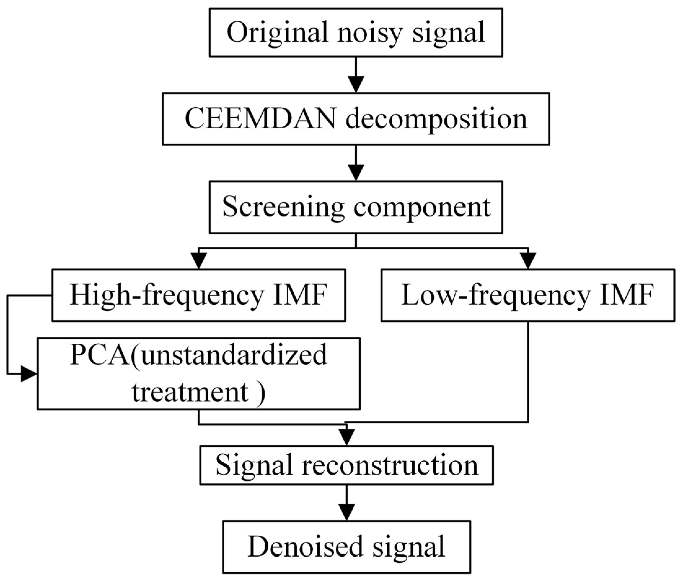
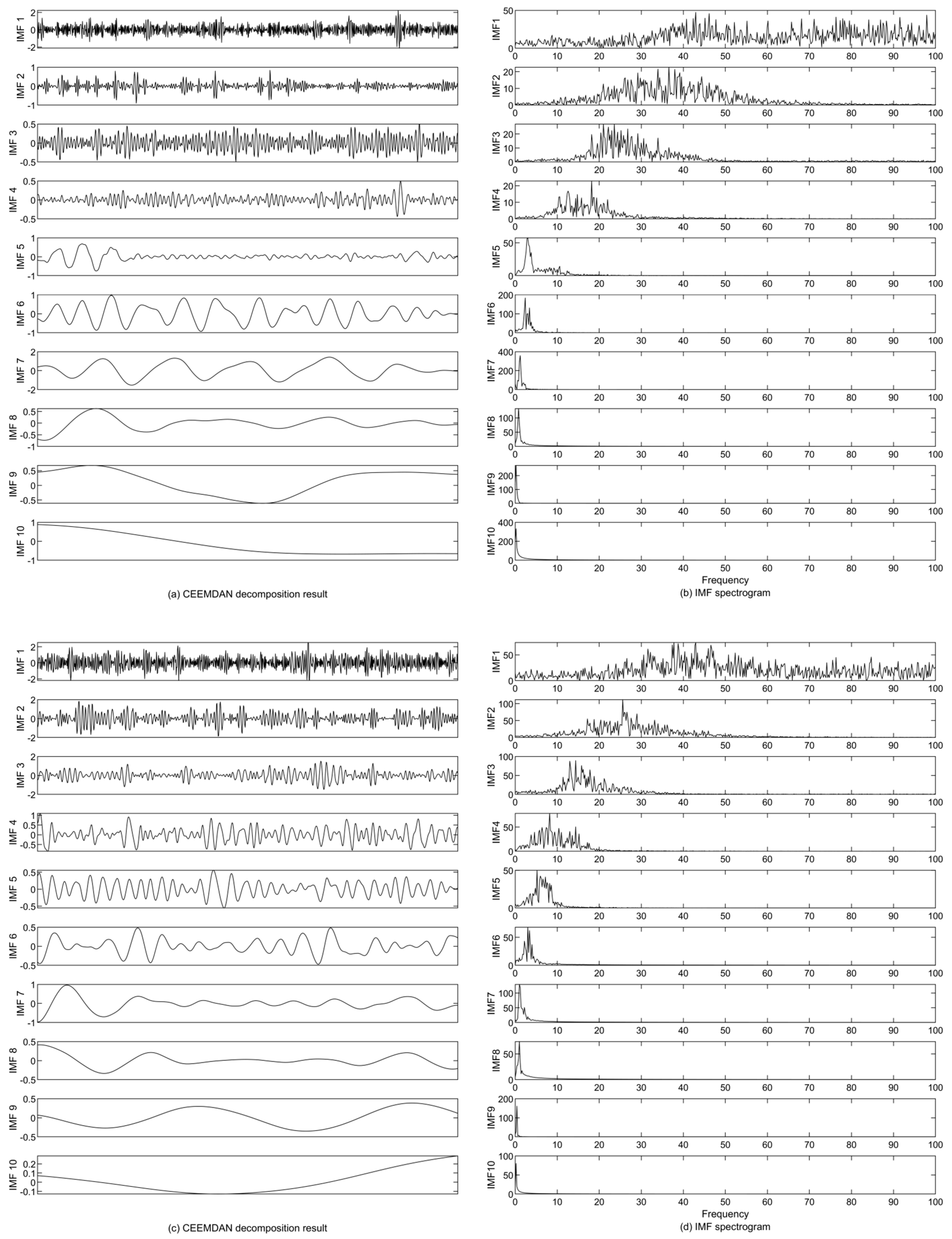
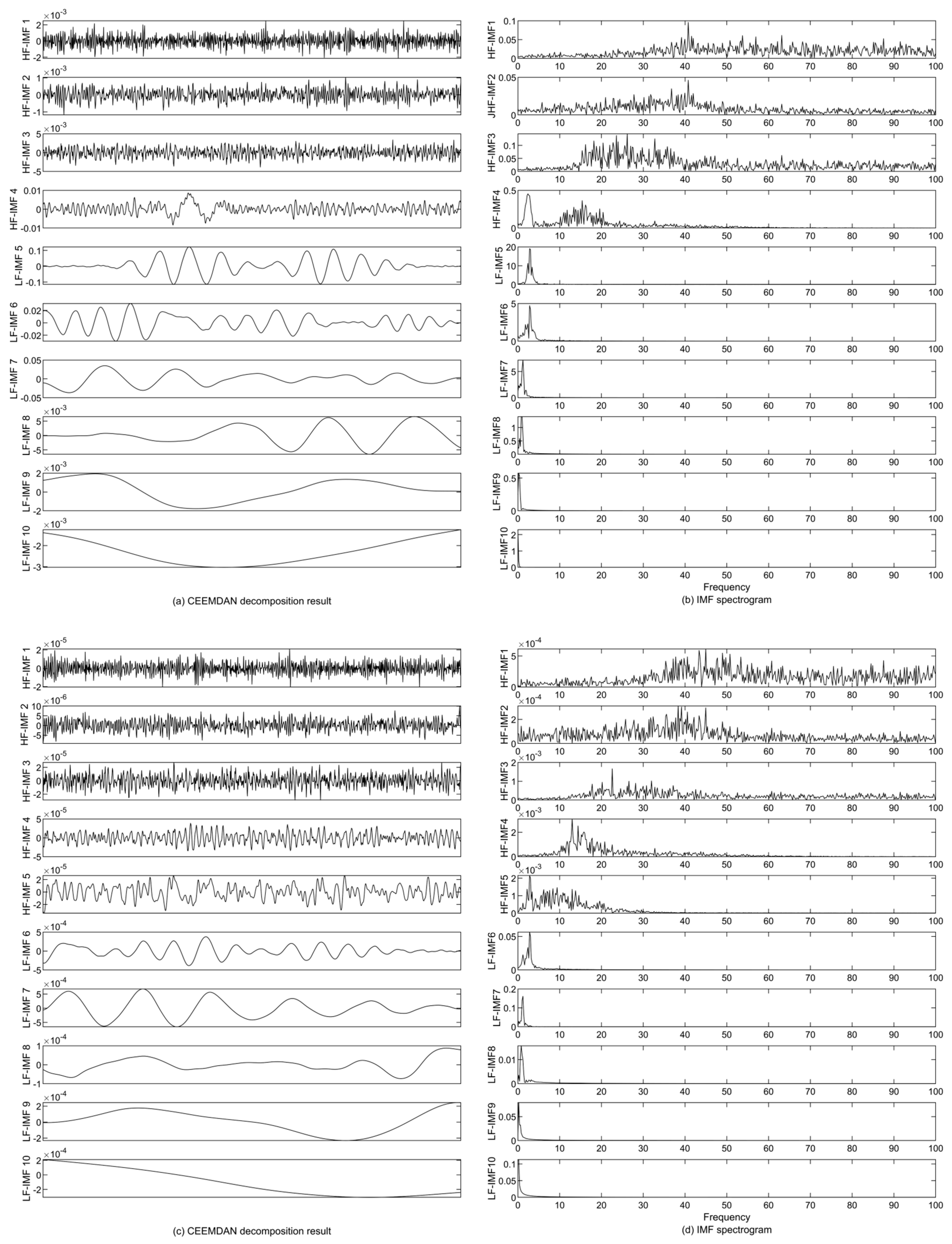
2.5.1. CEEMDAN-NSPCA Denoising Algorithm

The interpretation of the feature dimensions in PCA is somewhat ambiguous, lacking the very clear explanation of the original sample features. Non-principal components with small variance may still hold important information about differences among samples. Consequently, dimensionally reducing and discarding these components could impact subsequent analyses directly. If there is noise in the signal, especially the noise signal with a small standard deviation, it may be amplified in the process of standardization. This is because the standardization process is based on the standard deviation; the smaller the standard deviation, the more concentrated the data distribution and the better the central trend. The larger the standard deviation, the more dispersed the data distribution and the worse the central tendency, and when the standard deviation is small, even small noise may be significantly amplified after standardization. Therefore, the standard deviation is used to determine whether the signal needs standardized processing, and the standard deviation of 0.1 usually means that the data is less discrete. In this paper, the signals containing noise are all less than 0.1, and no standardized processing is required. Generally, the low-frequency component contains most of the energy and main information in the signal, and the high-frequency component contains the details and noise in the signal. By retaining the low-frequency component, the main information can be ensured such that the main information is not lost, and the noise removal of the high-frequency component can effectively remove the noise of the details. Therefore, a denoising algorithm is proposed in the flowchart in Figure 2 based on the combination of CEEMDAN and PCA without standardized treatment (CEEMDAN-NSPCA) to acquire the information. The IMF components through CEEMDAN with high-frequency IMF components are selected for the following dimensional reduction by PCA to preserve as much of the effective information as possible. The principal component contribution rate is defined as the variance of one principal component to the sum of variances, and it is used to measure the principal component’s contribution. The cumulative contribution rate of 0.85 is applied in this work. Finally, the denoised signal is reconstrued by the reserved principal components (orthogonalized IMF components) and the remaining low-frequency IMF components.

2.5.2. CEEMDAN-IWT Denoising Algorithm

Threshold selection is a key factor affecting the performance of wavelet denoising methods. If the threshold is too small, the processed signal will contain too many noise-dominated wavelet components against the purpose of denoising. On the contrary, if it is too large, partial signal components will be discarded and cause apparent signal distortion after reconstruction. In addition, these wavelets with small coefficients indeed carry the information at a higher frequency range, making them relevant for high bridge modes. The optimal threshold is determined by the improved wavelet threshold [33].
λ = σ 2 lg N , σ = median ω j . k 0.6745
where ω j , k is the k-jth coefficient after waveform decomposition, N is the signal length, σ is the signal variance, and λ is the threshold.
ω j , k = 0 , ω j , k , ω j , k < λ k ω j , k λ k , λ k = λ k 3
where ω j , k is the waveform coefficient of the reconstituted signal and λ k is the newly set threshold. The sym4 wavelet is used to decompose and denoise the high-frequency IMF component from CEEMDAN. To remove the noise components of the IMF component, the wavelet with a coefficient of less than this newly set decision threshold will be discarded, and the rest are retained. The final signal is reconstructed by the superposition of the recovered IMF component and the low-frequency IMF component decomposed by CEEMDAN through a wavelet transform. Figure 3 shows the flowchart of the proposed denoising algorithm of CEEMDAN combined with the improved wavelet threshold denoising algorithm (CEEMDAN-IWT).

2.5.3. Evaluation Index of Noise Reduction

The signal-to-noise ratio (SNR) represents the power ratio of signal PS to the noise Pn in logarithm form with a base of 10, which is used to evaluate the performance of the denoising algorithm.
S N R = 10 lg P s P n
where lg represents the logarithm with a base of 10.
In addition, the mean square error (MSE) can evaluate the differences between the true value xi and the predicted value yi.
M S E = 1 N i = 1 N ( x i y i ) 2

3. Simulation Examples

3.1. Configurations

The properties of a simply supported beam are given in Table 1. The beam damping property is neglected in this section and the following three sections (Section 3.2.1, Section 3.2.2 and Section 3.2.3). Its first three natural frequencies are 4.0202 Hz, 16.0850 Hz, and 36.1911 Hz. The beam is discretized by 25 equally long beam elements.
The properties of the vehicles [41] are given in Table 2. The natural frequencies and damping ratios of this two-DOF vehicle are mostly (2.3884 Hz, 0.0365) for the pitch motion and mostly (3.1832 Hz, 0.0413) for the bounce motion. The natural frequency and damping ratio of the one-DOF vehicle are (1.1254 Hz, 0.0283).
To ensure all vehicles vibrate adequately before entering the bridge, a 125 m long Class A (very good) road profile is generated. This road profile covers the bridge and two regular road parts (50 m) at both bridge ends. A 5 m long Class A road segment is plotted in Figure 4, as well as Class B (good) and Class C (average) road segments.
For the tractor with the three trailers travels at a velocity of 5 m/s (18 km/h), the displacement responses of the three trailers’ contact points are plotted in Figure 5a while traveling on the beam. The corresponding two residual accelerations between consecutive contact points are plotted in Figure 5b. By using a Hann window with a size of 128 and an overlap ratio of 99% under the sample frequency of 200 Hz, the STFT of the acceleration residual between the first two trailers (u1 and u2) is plotted in Figure 5c. There are peak ridges marked as red dashed horizontal lines along the first two beam natural frequencies (4.0202 Hz and 16.0850 Hz). The third ridge is located around 33 Hz, which is slightly lower than the third natural frequency (36.1911 Hz). Additionally, at the third natural frequency, the magnitudes of the STFT components are lower than those at this peak ridge, which indicates that the beam is not adequately excited at this frequency. Despite the peak ridge frequency of around 33 Hz not being closely aligning with the natural frequency, it could still be effectively utilized to extract a promising third mode shape in Figure 5.

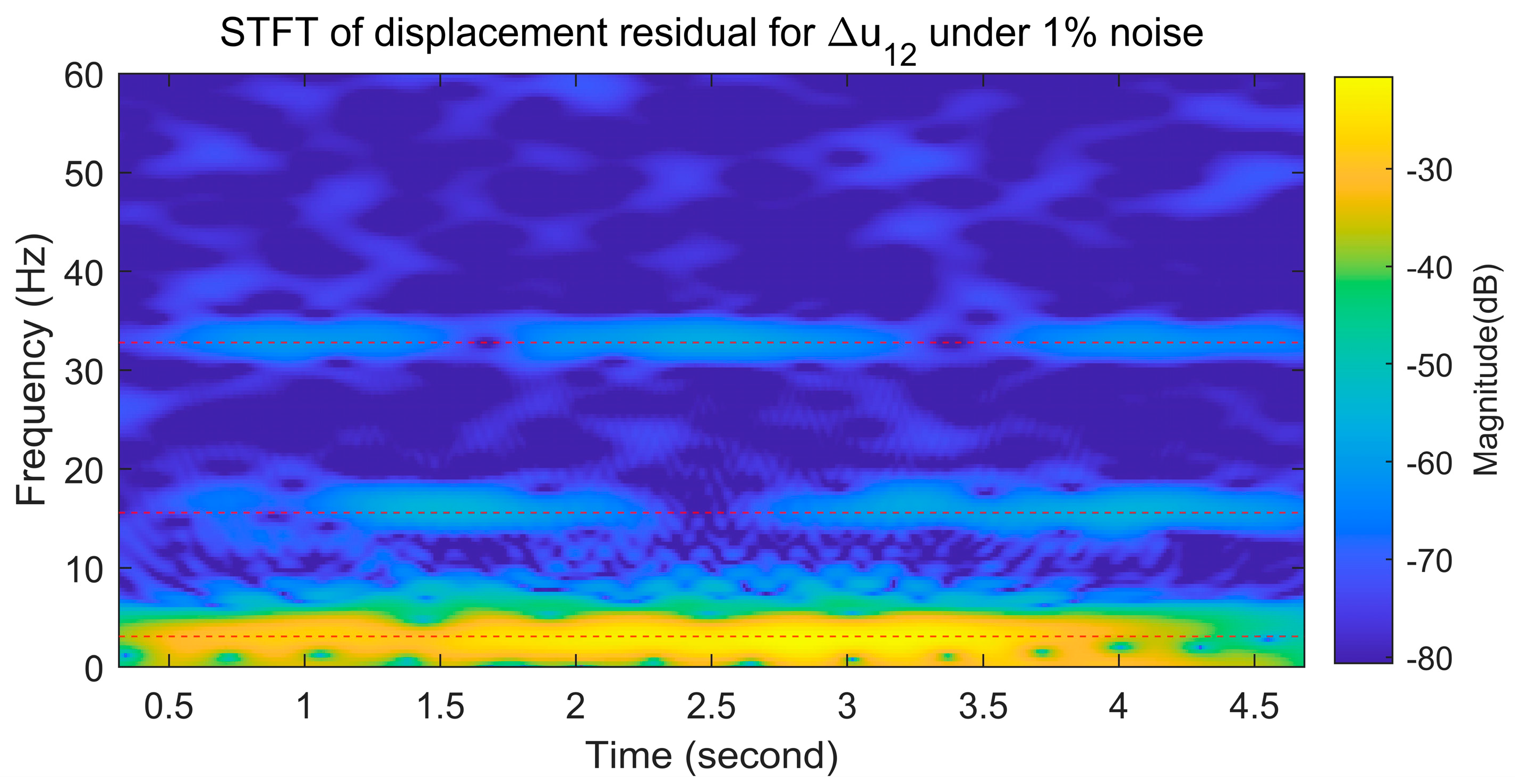
3.2. Residual STFT-Based Mode Shape Extraction

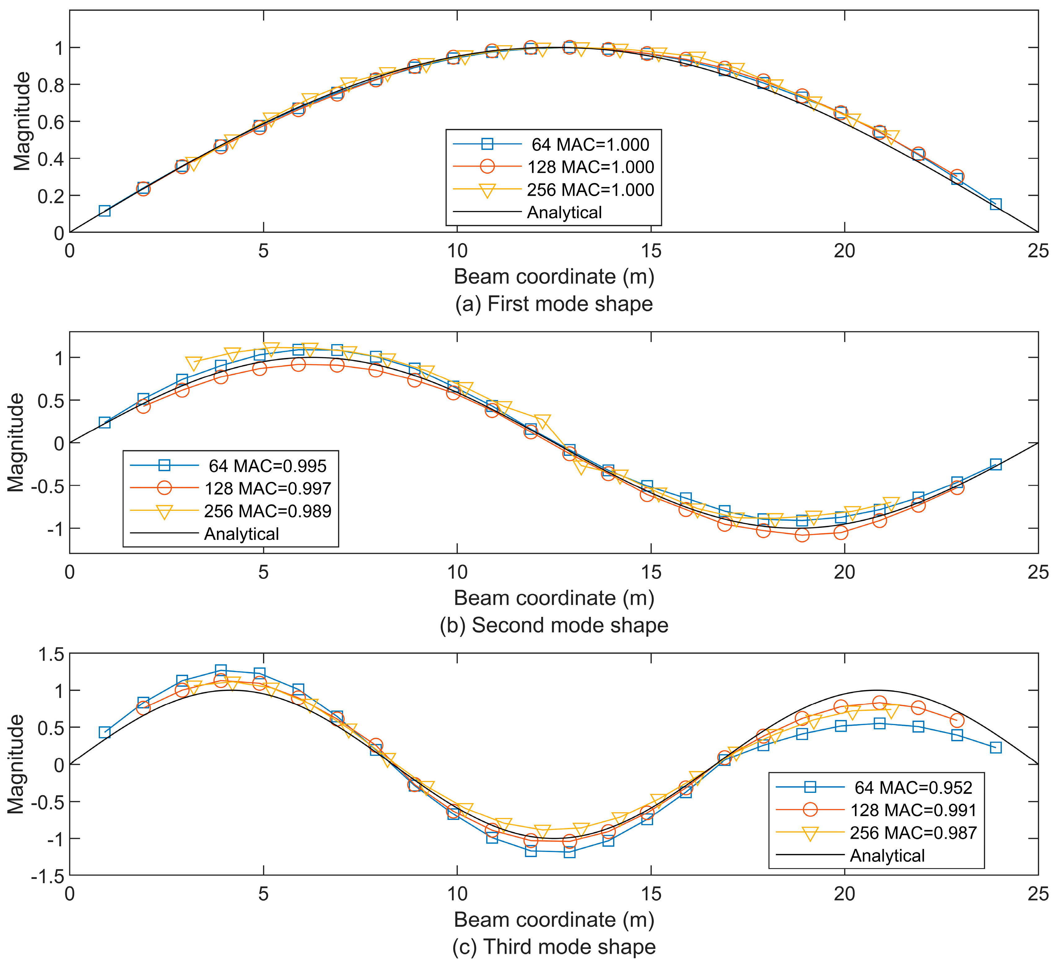
3.2.1. Effect of Window Size

In this section, the Hann window is used with three different sizes of 64, 128, and 256 with an overlap ratio of 99% to investigate the effect of window size under the sample frequency of 200 Hz. Meanwhile, the modal assurance criterion (MAC) [43] values is provided for the evaluation of the estimated mode shape (ϕe) with reference to the analytical one (ϕa).
As Figure 6 shows, the first three beam modes could fit well with the analytical ones. (All corresponding MAC values are larger than 0.91.) However, there are still some differences among the estimated mode shapes from these window sizes. Using a larger window size results in the loss of longer signal segments at the beginning and end. So, the window size of 64 could provide the longest mode shapes (from 1.0 m to 24.0 m of the beam length). Meanwhile, the window size of 256 could only provide the shortest mode shapes (from 3.5 m to 21.5 m of the beam length). However, for the second and third mode shapes, the window size of 64 contains a slightly larger deviation from the analytical ones when compared to the other two window sizes, even if the MAC values are larger than 0.95. In other words, a sufficient window size should be used to guarantee that the necessary information is contained [12]. The window size of 128 could be a balanced option, providing mode shapes from 2.0 m to 23.0 m along the beam and small deviations on the mode shapes, similar to the window size of 256. Then the Hann window with a window size of 128 and an overlap ratio of 99% is applied in the following sections.

3.2.2. Effect from Vehicle Velocity

As the derivations in Section 2.1 indicate, the residual responses between the contact points contain three main frequency components, including the driving frequency (2jπVe/L) and the two shifted frequencies (ωjjπVe/L and ωij + jπVe/L) centered at the beam natural frequency (ωj). So, the velocity (Ve) is critical to the distributions of these frequencies. Three different velocities are used including the slow speed of 2.5 m/s (9 km/h), the intermediate speed of 5 m/s (18 km/h), and the relatively high speed of 10 m/s (36 km/h) with the roughness profile of Class A.
When the tractor with the trailers moves on the bridge with different velocities, the duration varies as 10 s for the velocity of 2.5 m/s, 5 s for the velocity of 5 m/s, 2.5 s for the velocity of 5 m/s, and 2.5 s for the velocity of 10 m/s. A longer duration could provide more response data to the STFT. However, the ratio qj = jπVe/(j) in the contact point’s response expressions (Equation (7)) will decrease with the lower velocity and then reduce the contribution from the components (ωijπVe/L and ωi + jπVe/L) about the beam natural frequencies. As shown in Figure 7, all extracted first and second mode shapes using these three velocities are very close to the analytical ones. There are some moderate deviations around the peaks of the third mode shape, especially when using the lower velocity (2.5 m/s). As a contrast, the relatively high speed of 10 m/s could excite the beam from higher frequencies. However, due to it having the shortest duration among the three velocities, only the beam mode shapes from 3.5 m to 21.5 m of the beam length could be extracted using STFT. It is similar to using a larger window in the previous section. Therefore, a medium velocity of 5 m/s is recommended and used in the following work.

3.2.3. Effect of Road Roughness

Even if the bridge surface roughness in the contact point’s response could be eliminated by using the residual response between the contact points, it is assumed that the magnitude of roughness (ur) in the term [ ω v , i 2 u r ( V e ( t t i 1 ) ) + g ] in Equation (5) is much smaller than gravity (g) and could be ignored. However, when the roughness is increasing, its contribution should be explored to validate the above assumption. So, in addition to the Class A road profile in Figure 4, Class B and Class C road profiles are used to explore the effect of road roughness. For the velocity of 5 m/s, the resulting mode shapes are plotted in Figure 8. For all three road classes, the first three modes could match the analytical ones well. All the MAC values larger than 0.96 could indicate that the roughness level has no obvious effect on the mode shape extraction.

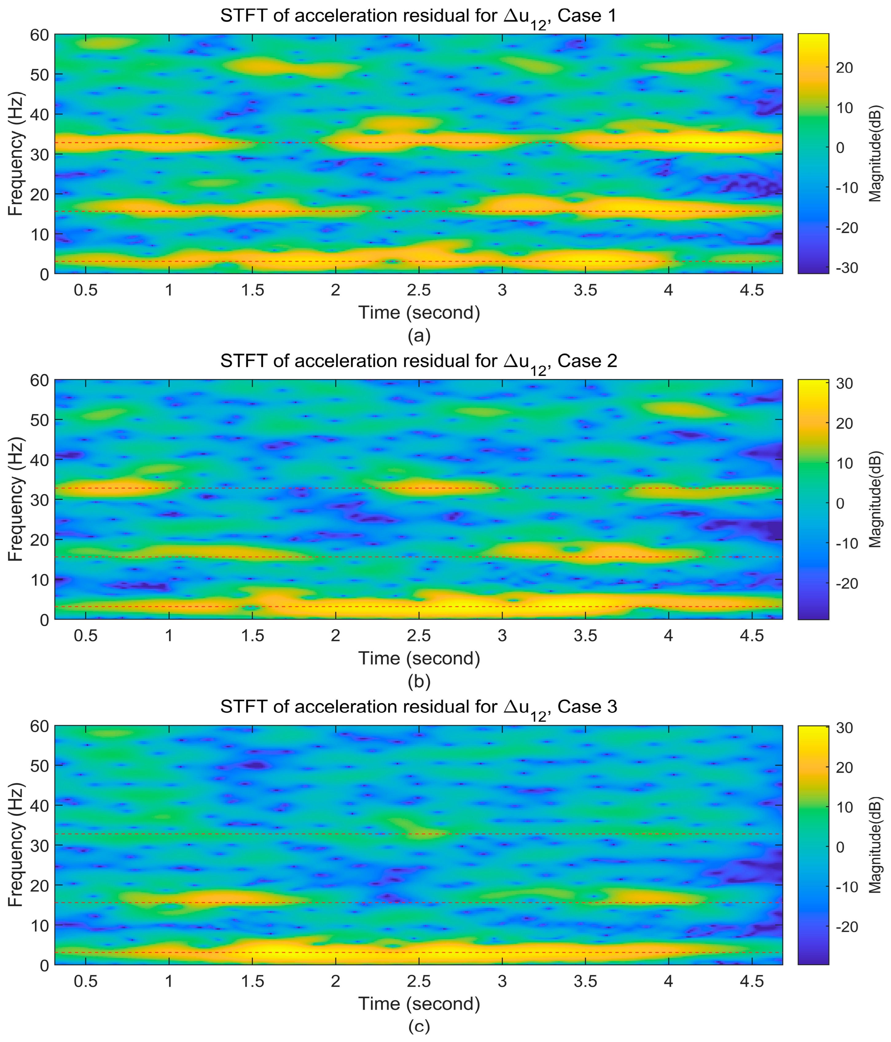
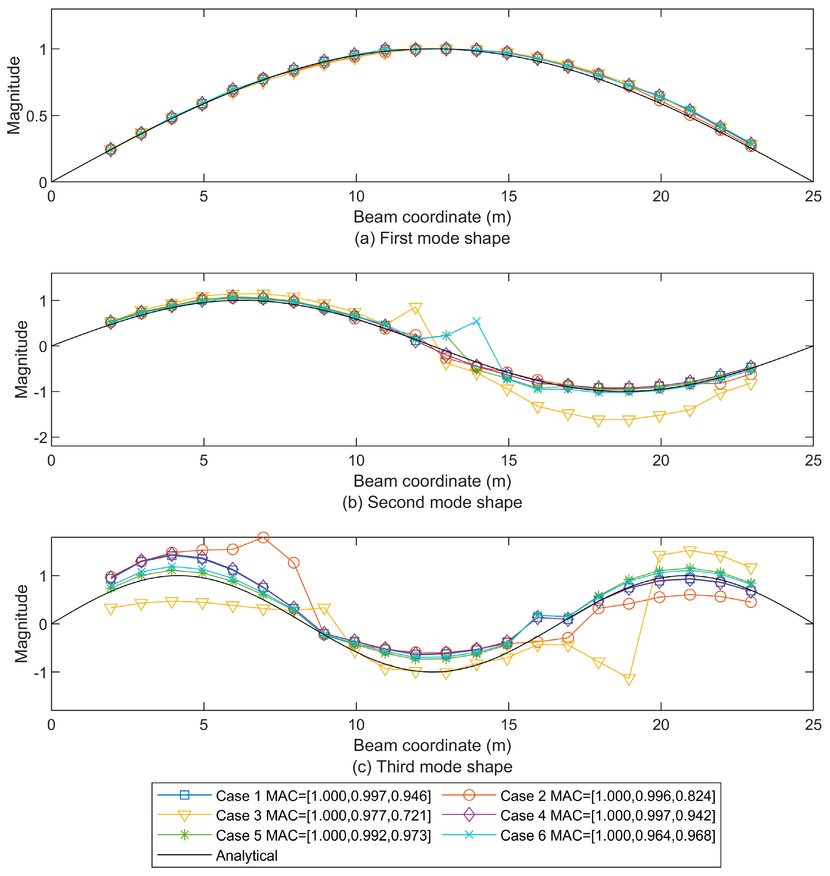
3.2.4. Effect from the Beam Damping Property

In the field of moving load problems, especially when identifying bridge modal properties, most previous works considered the damping property of the vehicles rather than the bridge itself. However, beam damping could also impact its dynamical characteristic in this limited duration [22,44]. As shown in Equation (25) with the Rayleigh damping assumption [45],to investigate the beam damping effect on mode extraction, there are six damping cases, including three cases with only the stiffness damping coefficient (ri = βEI) and three cases with both the mass damping coefficient re = αm and the stiffness damping coefficient ri = βEI in this section, as shown in Table 3 as well as the corresponding damping ratios for the first three modes.
With the velocity of 5 m/s and the road profile of Class A, the STFT of the acceleration residual between the first two trailers (u1 and u2) is plotted in Figure 9 for the first three cases (Case1 to Case 3). Compared to Figure 5c for the undamped case, at the second and especially the third natural frequencies, the peak ridges are less prominent from all the three cases. This indicates that the existence of beam damping could suppress the dynamical response, especially on the peaks near the natural frequencies.
Moreover, to consider the effect of traffic flow, two groups of 10 vehicles with an equal space of 5 m are added to the three cases. The vehicles in both groups share the parameters of the one-DOF vehicle in Table 2 and their velocity. However, one vehicle group has the same moving direction as the tractor (toward the right), and the other vehicle group moves in the opposite direction (toward the left). So, when the tractor with three trailers enters and leaves the beam, there are well-spaced vehicles moving on the bridge all the time. The extracted mode shapes are plotted for all cases without traffic flow in Figure 10 and their corresponding cases with traffic flow in Figure 11.
At the first mode, all cases of different damping coefficients, without or with traffic flow, have the accurate extracted mode shapes. The second mode shapes extracted from these cases without or with traffic flow also approximate the analytical ones with a MAC value of larger than 0.95 except for Case 6, which has the largest second modal damping coefficient (ξ2 = 0.0404). The evident deviations at the third mode are caused by beam damping. With the smallest third modal damping ratio (ξ3 = 0.0114), Case 1 (without traffic flow) and Case 4 (with traffic flow) could provide well-fitted mode shapes like the undamped case in Figure 7, with MAC values of 0.946 and 0.943, respectively. However, due to the involvement of internal damping, the modal damping ratio will be larger at the higher mode. With the third modal damping ratio (ξ3 = 0.0341), there are remarkable derivations from the analytical mode shape for Case 2 (without traffic flow) with a MAC value of 0.824. When traffic flow is taken into consideration, Case 5 could still provide the mode shapes with a MAC value larger than 0.92. When the third modal damping ratio comes to ξ3 = 0.0910, the mode shapes extracted from Case 3 (without traffic flow) are distorted with MAC values of less than 0.73. At the same time, Case 6 (with traffic flow) could keep the MAC values larger than 0.96.

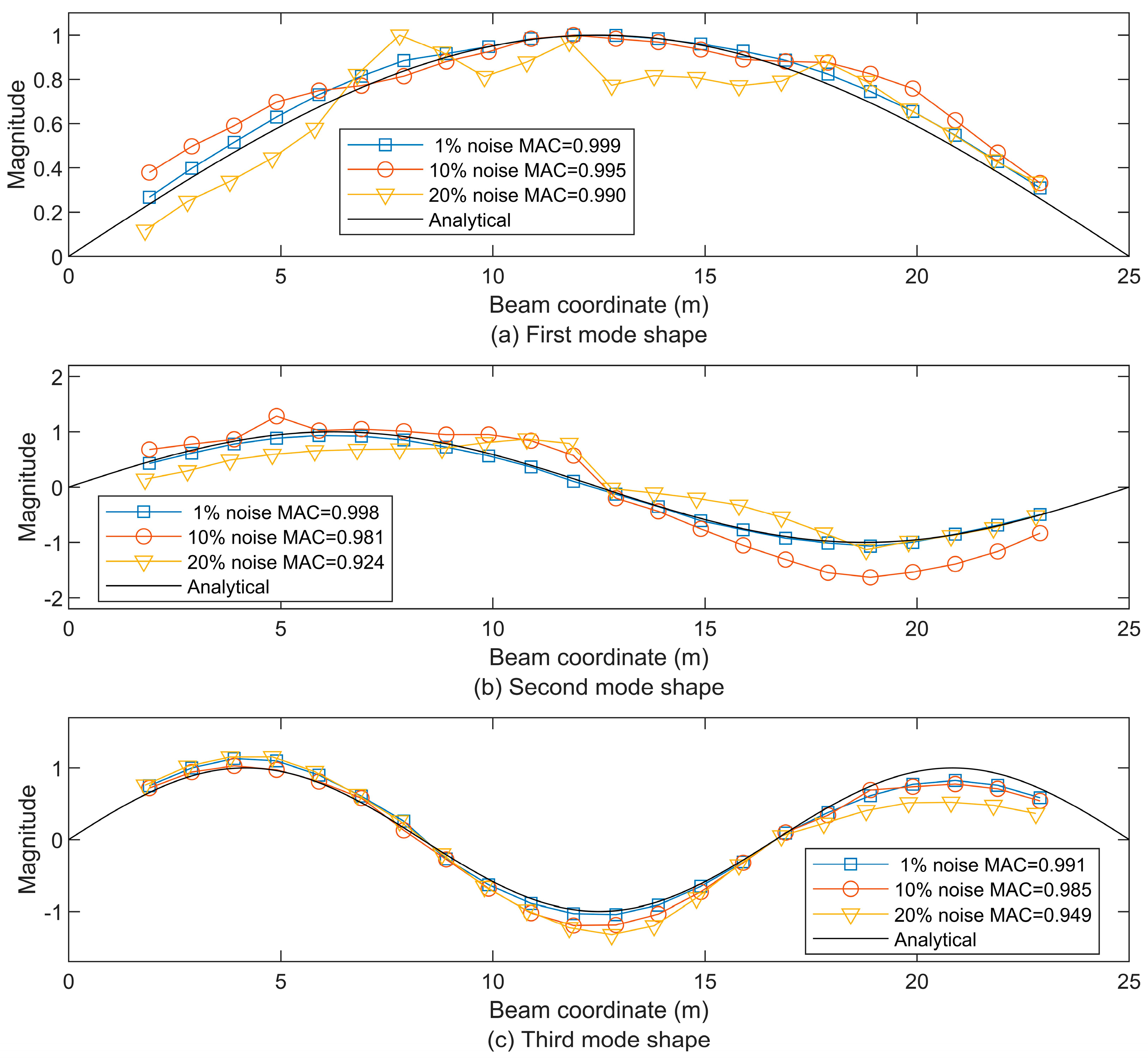
3.2.5. Effect of Noisy Disturbances

As shown in the definition of Equation (39), three white noises with levels of 1%, 10%, and 20% are added to the acceleration responses of the three trailers’ contact points to investigate the effect of noisy disturbances.
u ¨ n = u ¨ s + N l σ s R N
where the noisy acceleration u ¨ n is constructed from acceleration u ¨ s added to the uniformly distributed vector R N with the noise level Nl and standard deviations σs of u ¨ s .
With a velocity of 5 m/s and a Class A road profile, the undamped beam case from Section 3.2 is used. As shown in Figure 12, it is clear that the deviations of the mode shapes are boosted by the increasing noise level. Under 1% noise, the mode shapes are close to the undamped case in Figure 7 and could match the analytical ones. When the noise level increases to 20%, the corresponding MAC values could still be larger than 0.9. For the noise levels of 10% and 20%, the large derivations from the analytical mode shapes appear mainly at the peaks.

3.3. Mode Shape Extraction Using Displacement Approximation of Contact Points

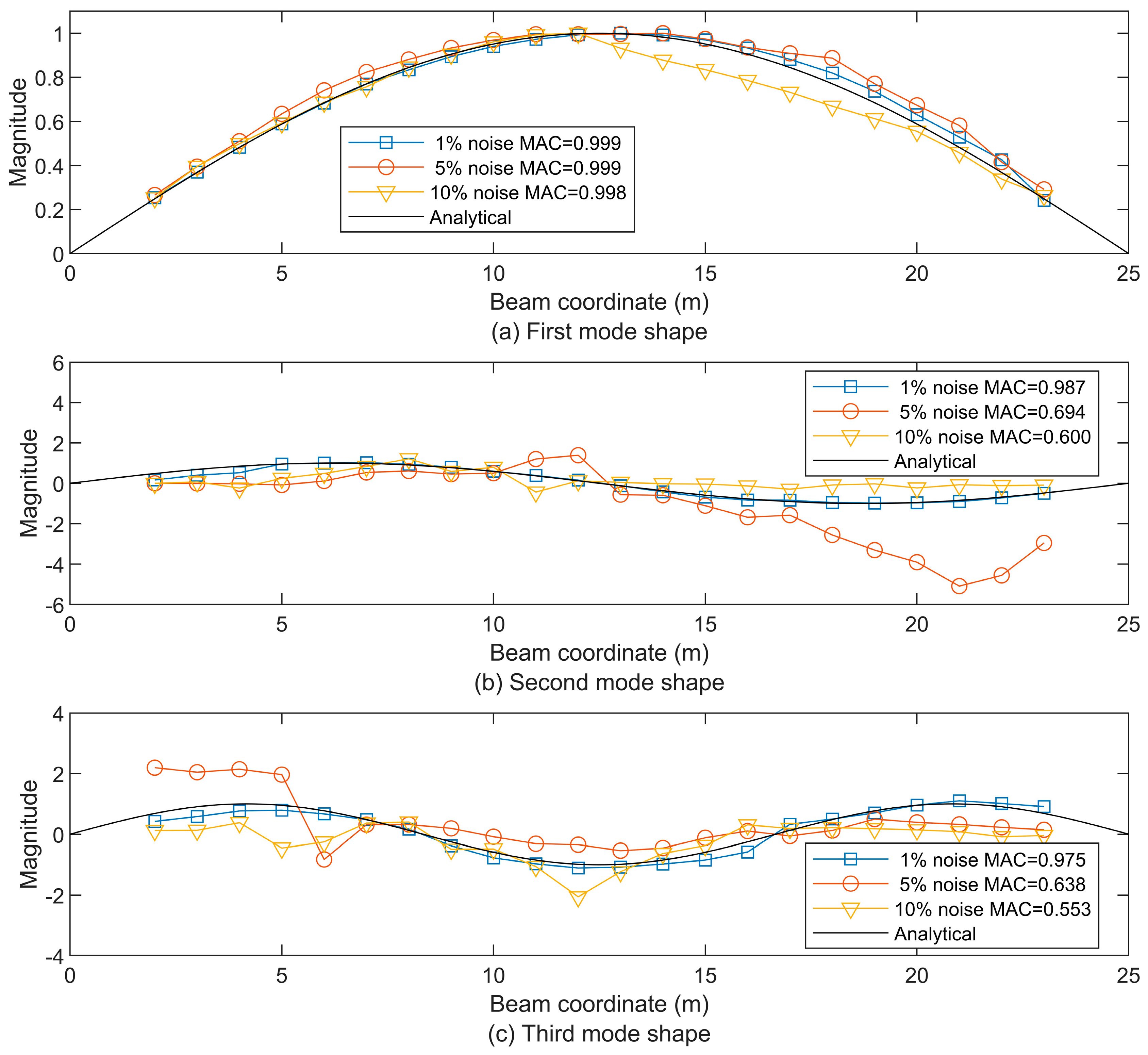
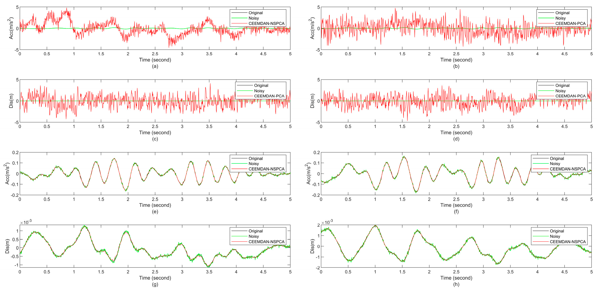
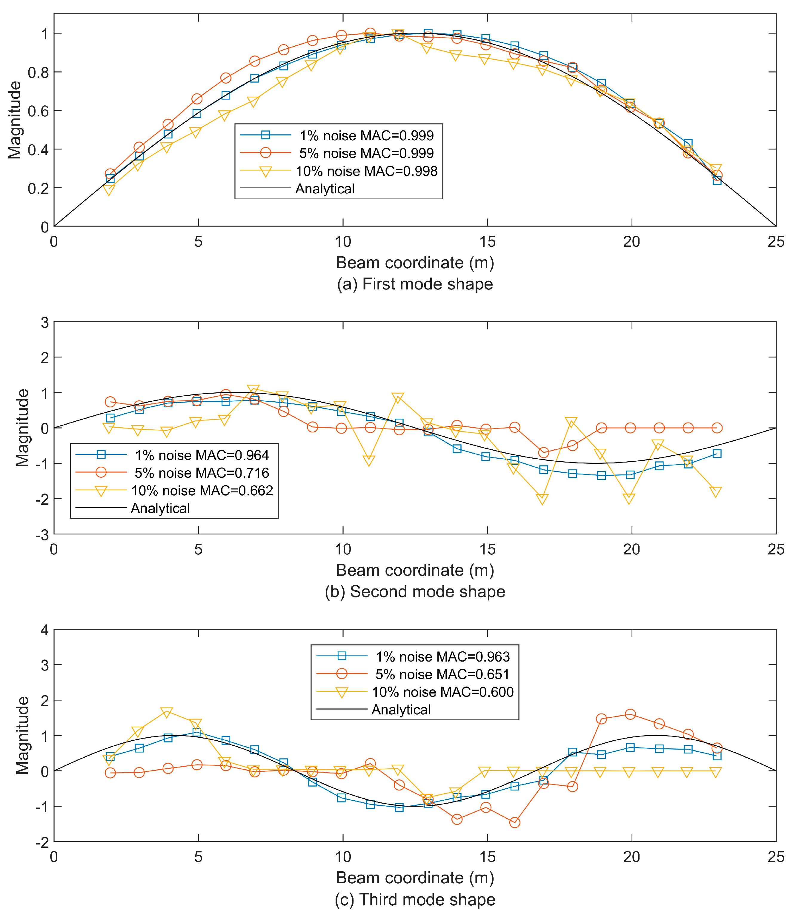
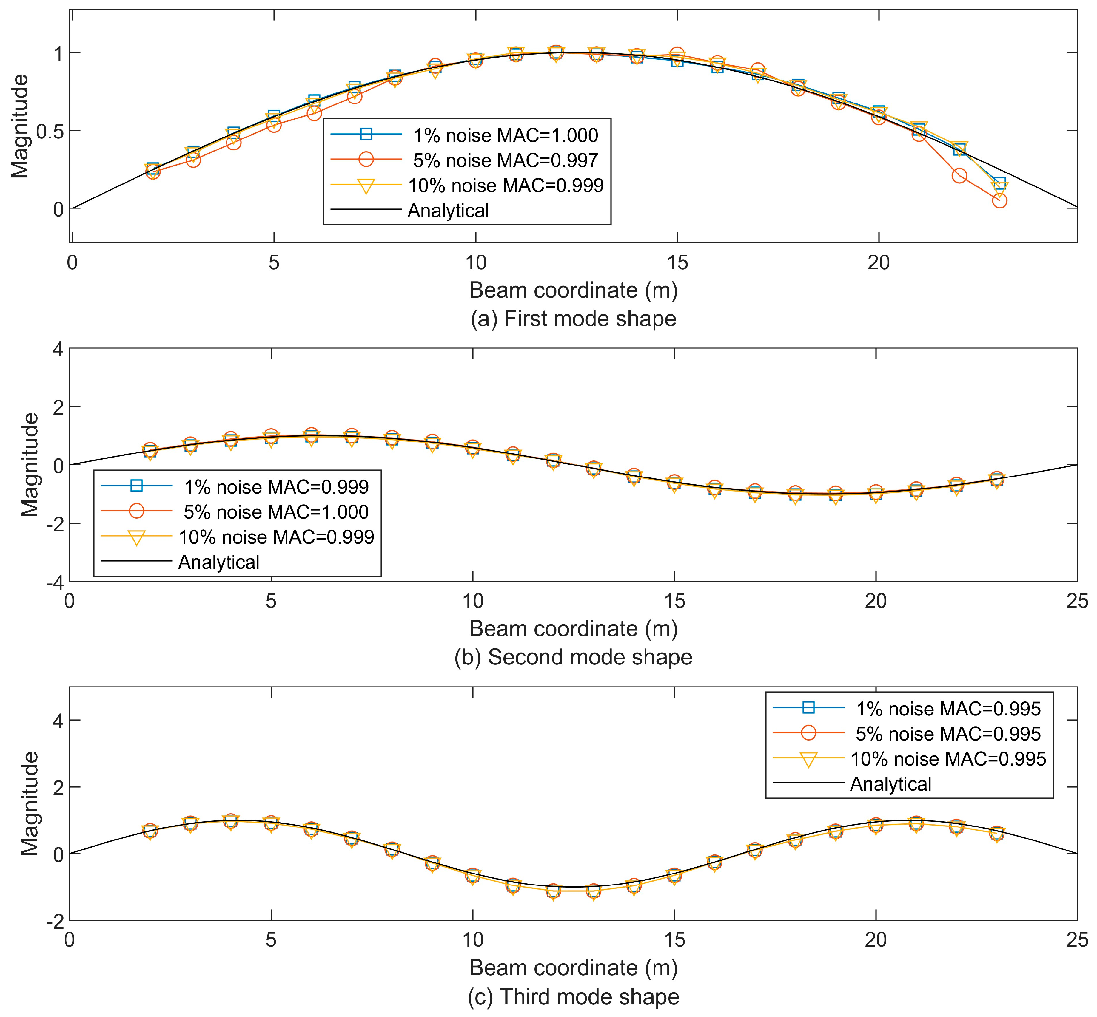
3.3.1. Effect from Noisy Disturbance

In the previous numerical examples, the responses of the contact points could be obtained easily from Equation (30). By contrast, in practice, an attempt is made to measure the responses of the contact points from the lower part of the vehicle’s suspension. Alternatively, they can be approximated from the measured vehicle responses [13] without considering the vehicle’s damping.
u ¨ c = u ¨ v + u v ω v 2 ( Δ t ) 2 , ω v 2 = k v m v
where the four over-dots denote the fourth temporal derivative of the vehicle’s response (uv). Once the vehicle’s response is utilized to calculate the response of the contact point, the noise level from the vehicle response is amplified prominently on the resulting contact point’s response through the twice finite difference operation on u ¨ v with a small Δt. Then, its displacement response could be expressed as follows:
u c = u ¨ v ω v 2 + u v
where the coefficients ( 1 ω v 2 and 1) of the acceleration u ¨ v and the displacement u v could be considered as the weights between them on the resulting contact point’s displacement. According to the previous works that used the acceleration [11,12,13,14,15,16] and displacement [14] of the vehicle, both quantities could be utilized to extract the mode shapes. As shown in Equations (9)–(12), like the contact points’ accelerations, their displacements could also be used for the extraction of the mode shapes. Moreover, compared to using acceleration only as in Equation (40), using both acceleration and displacement could avoid the huge amplifying effect from the finite difference operations.
The performance of mode shape extraction using this displacement approximation is investigated under the noise levels of 1%, 5%, and 10% on the accelerations and displacements of the vehicles. As shown in Figure 13, the first mode shapes under all three noise levels fit very well with a MAC value close to one. However, the influence of noise becomes obvious at the second mode shapes. Under 1% noise, the MAC value of the second mode shape could be kept over 0.97. Meanwhile, the second mode shapes under 5% and 10% noise are distorted, with MAC values of 0.694 and 0.638. Only the third mode shape under 1% noise is reasonable. The third mode shape at 5% noise is also poor, with a MAC value of 0.638, and the third mode shape extracted at 10% noise is meaningless, with a MAC value of less than 0.6. Compared with the STFT of the acceleration residuals in Figure 5c, there is not much energy distributed on the higher frequencies for the displacement residual in Figure 14. Except for the peak ridge along the first natural frequency, the other peak ridges at the higher frequencies are small compared to the acceleration responses. Consequently, the mode shapes extracted using the displacement approximation of contact points exhibit significantly more noise disturbances compared to those in Figure 12, particularly in the second and third mode shapes when subjected to noise levels of 5% and 10%, as illustrated in Figure 13.
Considering the poor performance under noisy disturbances in the above cases, it is crucial to denoise the signal before extracting the mode shape. So, the two proposed signal denoising algorithms, CEEMDAN-NSPCA and CEEMDAN-IWT, are evaluated for their effectiveness in enhancing mode shape extraction using displacement approximation of contact points. Additionally, two denoising algorithms, CEEMDAN-PCA and IWT, are applied as references.

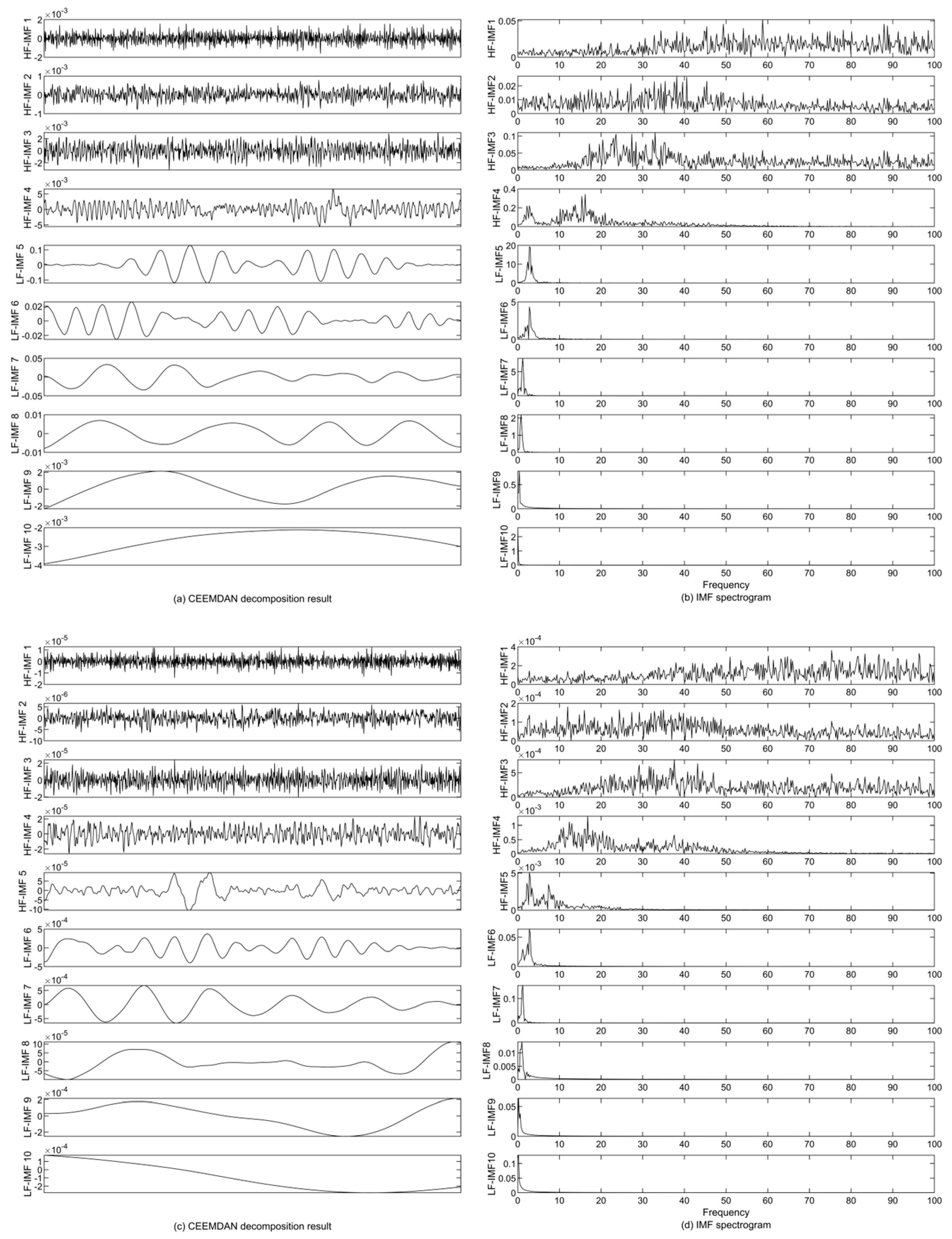
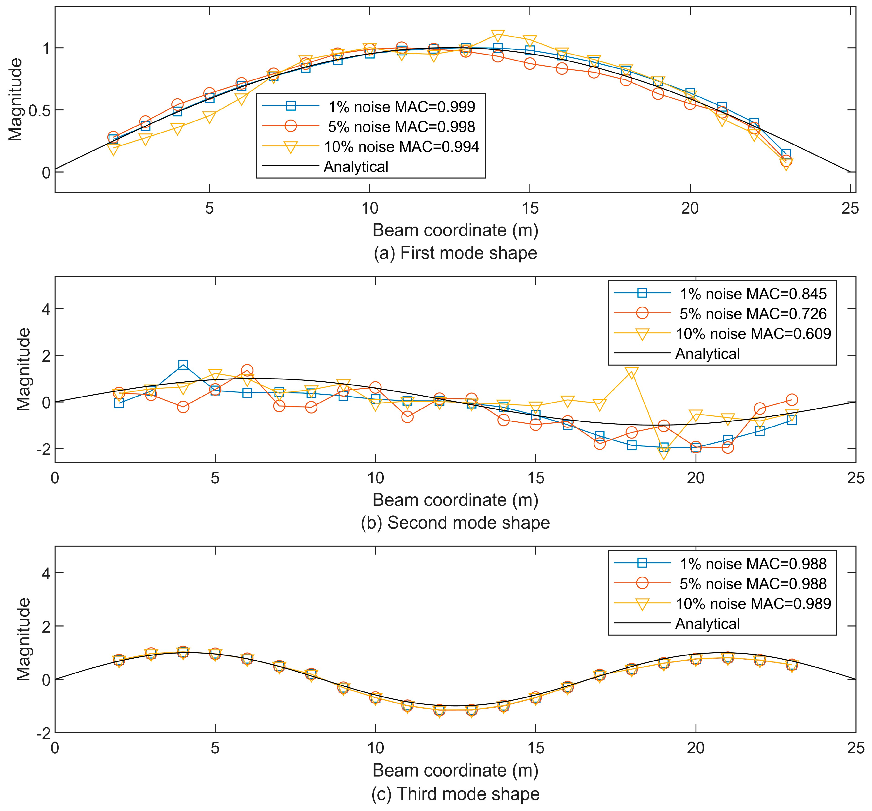
3.3.2. Mode Shape Extraction with CEEMDAN-NSPCA

At a noise level of 10%, the residual accelerations (Δü1,2) between Vehicle 1 and Vehicle 2 are decomposed by CEEMDAN with a standard deviation of 0.0577. Comparing the original IMF components from CEEMDAN in Figure 15 with the orthogonalized IMF components by PCA in Figure 16, the residual displacement and residual acceleration amplitude after PCA fluctuate greatly. The spectrum of all components is altered vastly for both acceleration and displacement through PCA, and the amplitude increases. Moreover, according to the cumulative contribution rate of 0.85, the residual acceleration of IMF-1 to IMF-7 and the residual displacement of IMF-1 to IMF-6 will be discarded to lead to the loss of high frequency contents. In Figure 16, IMF-1 to IMF-4 are high-frequency components, and IMF-5 to IMF-10 are low-frequency components as seen in the CEEMDAN-NSPCA flow charts. As shown in Figure 2, the high-frequency component was selected for PCA. Meanwhile, the high-frequency and low-frequency IMF components from CEEMDAN and the original residual displacement (Δu1,2) are IMF-1~IMF-5 and IMF-6~IMF-10, and the standard deviation is 5.119 × 10⁻⁴. For both residual accelerations and displacements, it is evident that their IMF components (IMF-1 to IMF-4 and IMF-1 to IMF-5) with a high frequency contain contents with the higher frequency range, which cover the second (16.0850 Hz) and third modes (36.1911 Hz).
Instead of involving all components, only high-frequency IMF components are selected for PCA in the CEEMDAN-NSPCA process, including IMF-1 to IMF-4 for acceleration and IMF-1 to IMF-5 for displacement. All these orthogonalized IMF components by PCA are marked in Figure 17. It is easy to find that the method effectively suppresses the noise of the high-frequency components of acceleration and displacement and retains the effective information. With the same cumulative contribution rate of 0.85, the orthogonalized components are picked for the final signal’s construction, including HF-IMF-1 to HF-IMF-3 for acceleration and HF-IMF-1 to HF-IMF-3 for displacement, which contain the higher-frequency contents as mentioned above.
The denoised signals by CEEMDAN-PCA and CEEMDAN-NSPCA are plotted in Figure 18. The SNR and MSE of noise-contaminated and denoised signals are provided in Table 4, wherein Δü1,2 and Δü2,3 are the residual accelerations between consecutive contact points. The smoother denoised signals by CEEMDAN-PCA show remarkable deviations away from the original signals rather than the denoised ones by CEEMDAN-NSPCA, which introduces more noise, resulting in the decline of signal smoothness. For Δü1,2 the acceleration and the signal-to-noise ratio (SNR) increase by approximately 180.85%, while the corresponding mean square error (MSE) reduces by approximately 99.99%. For Δu1,2 the displacement and the SNR increase by approximately 132.33%, and the corresponding MSE decreases by approximately 99.99%. After CEEMDAN-PCA denoising, the SNR of the residual acceleration and displacement polluted by noise decreases sharply, and the MSE increases sharply. It can be clearly found that standardizing a signal with a smaller standard deviation introduces more noise, and the more the SNR decreases, the more the MSE increases. The failure at this moving load’s vibrated responses may be caused by putting all the IMF components into PCA indiscriminately. In Figure 15, the IMF components concentrated on higher frequencies have smaller amplitudes. So, the information carried by these IMF components is easily drowned after PCA. By contrast, the SNR and MSE of the denoised signal by CEEMDAN-NSPCA receive obvious improvement. The IMF components are distinguished before PCA. The noise signal is decomposed through CEEMDAN, minimizing the mode aliasing, extracting the high-frequency component for principal component analysis, and retaining the low-frequency component to retain its information to the greatest extent. As shown in Figure 19, the extracted mode shapes from the denoised signals using CEEMDAN-PCA are seriously distorted and even worse than those from the noise-contaminated signals in Figure 13. By applying CEEMDAN-NSPCA, the extracted mode shapes could remain in acceptable profiles under the 10% noise level, as shown in Figure 20. The MAC values are 0.998, 0.662, and 0.600 for these three modes at the 10% noise level, while the corresponding MAC values are 0.998, 0.600, and 0.553 without noise reduction. Subsequently, the modal shapes extracted using CEEMDAN-NSPCA are closer to the analytical solutions compared to CEEMDAN-PCA. For the first mode, both are close to one. The second and third mode are improved by approximately 10.33% and 8.49%, respectively.

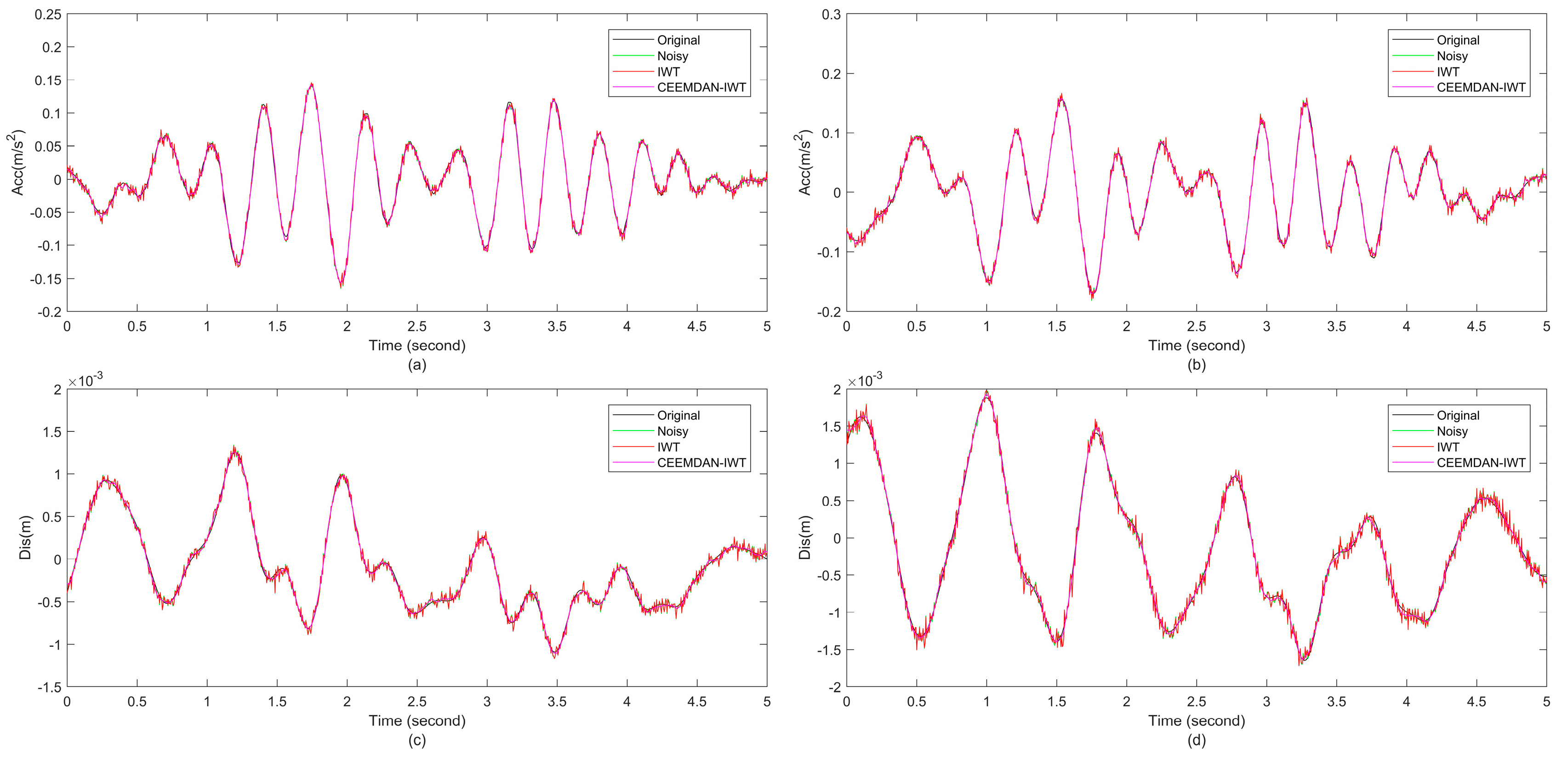
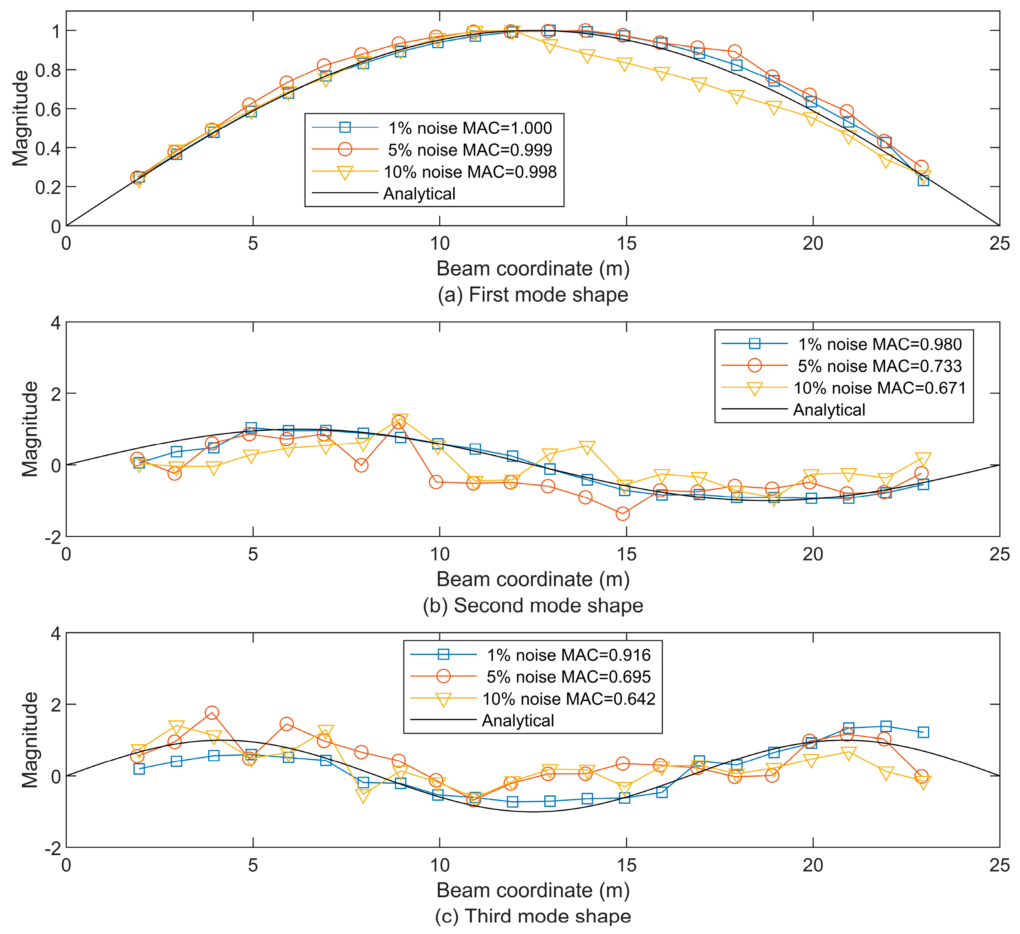
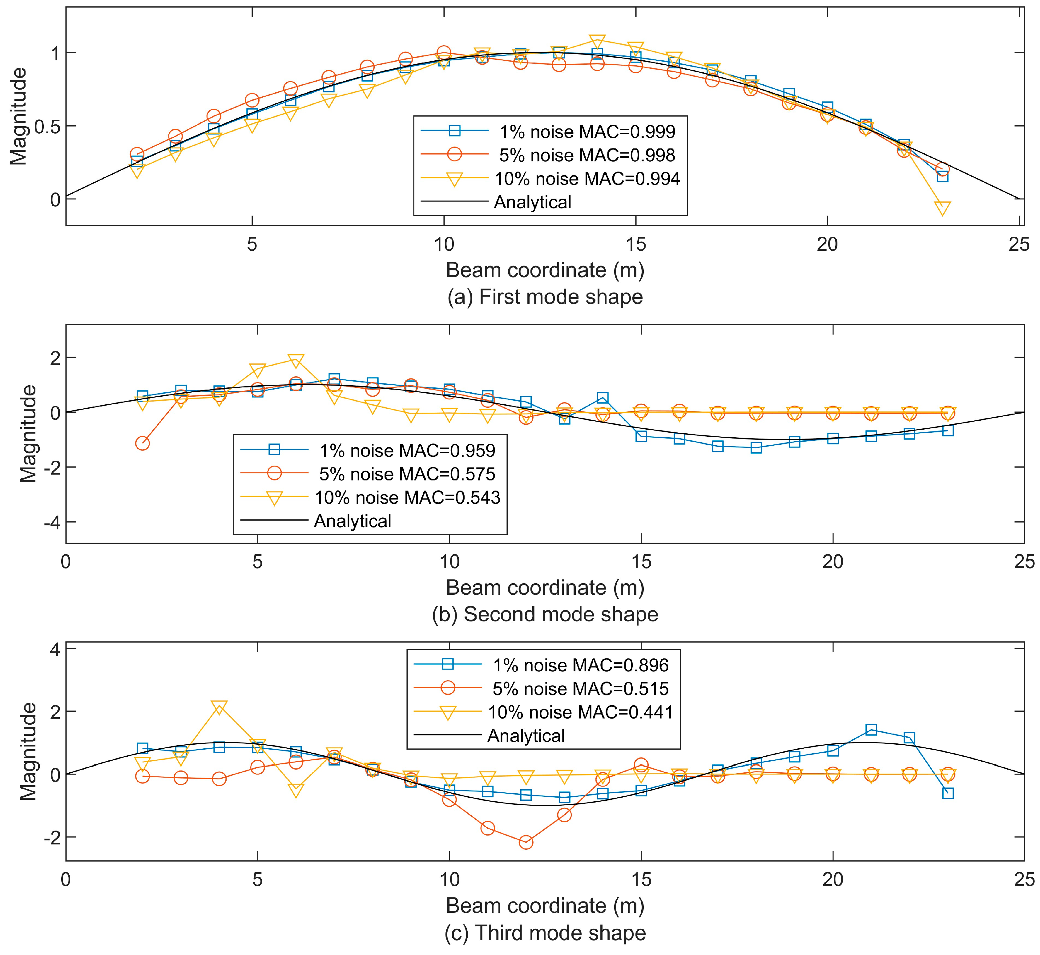
3.3.3. Mode Shape Extraction with CEEMDAN-IWT

Figure 21 illustrates the CEEMDAN of residual accelerations (Δü1,2) and residual displacements (Δu1,2) between Vehicle 1 and Vehicle 2 after wavelet denoising using the threshold function determined by the improved wavelet threshold at the noise level of 10%, in which the amplitude of the high-frequency IMF component and the low-frequency IMF component fluctuated slightly. According to SNR and MSE in Table 5, there is no significant change in acceleration or displacement before and after noise reduction, and the denoising effect of IWT is quite limited. At a noise level of 10%, for Δü1,2 the acceleration and its SNR increase approximately 29.26%, and the corresponding MSE is reduced by approximately 73.77%. For Δu1,2 the displacement and the SNR increase by approximately 36.15%, and the MSE decreases by approximately 35.75%. In CEEMDAN-IWT, an improved wavelet threshold function is used to determine the optimal threshold to properly retain these small-amplitude, high-frequency contents. The comparison of Figure 15 and Figure 22 reveals that all the wavelet-denoised high-frequency IMF components could still maintain concentrated frequency contents and effectively remove noise, particularly for IMF-1 to IMF-4 and IMF-1 to IMF-5 for both acceleration and displacement. Consequently, CEEMDAN-IWT could provide a better denoised signal than IWT, as shown in Figure 23 and Table 5. In Figure 24, under the 10% noise level, the first mode, which is well extracted and has a MAC value close to one, and the second and third modes, which have MAC values of 0.634 and 0.529, show little change. Subsequently, the modal shapes extracted using CEEMDAN-IWT are closer to the analytical solutions compared to IWT. For the first mode, both are close to one. The second and third modes are improved by approximately 15.11% and 22.87%, respectively. This indicates that while the IWT effectively filters noise from the high-frequency IMF components, it inevitably removes some low-frequency contents.
CEEMDAN-IWT could enhance the accuracy of the second mode shape under noise levels of 1%, 5%, and 10%, as shown in Figure 25. Moreover, in the lower-amplitude time–frequency region around the third mode, as shown in Figure 14, the extracted third mode shape exhibits good improvement. This indicates that both CEEMDAN-NSPCA and CEEMDAN-IWT can deal with the small-amplitude high-frequency signal fraction well, and CEEMDAN-IWT is better than CEEMDAN-NSPCA in terms of stability.

3.3.4. The Influence of Noise Interference at the Specified Frequency Band

By controlling the level of white noise (1%, 5%, 10%) and combining with a low-pass filter to generate three kinds of band-limited noises of 10 Hz, 20 Hz, and 50 Hz, the influence of noise frequency components on the modal recognition of vehicle vibration signals was systematically evaluated. The experimental results show that, as shown in Figure 26, Figure 27 and Figure 28, at the 10 HZ frequency component, the MAC is close to 1, verifying the robustness of this method at the 10Hz frequency component, which is highly consistent with the anti-interference requirements of the main frequency band in the actual bridge monitoring scenario.

4. Conclusions

This study aims to explore the extraction of modal shapes of beam bridges by using the residual responses between continuous vehicle contact points through STFT. To enhance the robustness and accuracy of modal shape extraction using the approximate expression of the contact points’ displacements under noisy disturbance, two novel denoising algorithms were developed. The proposed methodology provides an effective and practical approach for dynamic bridge analysis and damage detection, particularly under operational conditions involving moving vehicles.
(1)
Several key parameters were investigated, including window size, vehicle speed, road surface roughness, beam damping characteristics, and the influence of traffic flow. Among them, the damping characteristics of the beam are crucial to the performance of modal vibration mode extraction. A higher damping ratio (greater than 0.03) leads to modal shape distortion. The addition of traffic flow can amplify the beam response, thereby improving the accuracy of extracting modal shapes.
(2)
Two advanced denoising methods, CEEMDAN-NSPCA and CEEMDAN-IWT, were developed to enhance modal shape extraction under noisy conditions. CEEMDAN-NSPCA applies PCA-based dimensionality reduction to high-frequency components after CEEMDAN while preserving low-frequency content. CEEMDAN-IWT employs an improved wavelet thresholding strategy for denoising high-frequency components. Compared with conventional CEEMDAN-PCA and IWT denoising techniques, the proposed methods offer superior noise suppression while retaining essential micro-fluctuation characteristics. The results demonstrate that CEEMDAN-IWT achieves the highest accuracy and stability, particularly in the second and third modal shapes.

Author Contributions

Conceptualization, G.Q. and Q.W.; methodology, G.Q. and X.D.; validation, X.D.; writing—original draft preparation, X.D.; writing—review and editing, Gaundong Qiao and L.J.; visualization, X.D.; supervision, Q.W. All authors have read and agreed to the published version of the manuscript.

Funding

This research was is supported by the National Natural Science Foundation of China grant number 52008061, the Hainan Provincial Natural Science Foundation of China grant number 525MS044, 525RC705, and the Hainan Province Science and Technology Special Fund grant number ZDYF2022SHFZ353. And the APC was funded by the Hainan Province Science and Technology Special Fund grant number ZDYF2022SHFZ353.

Institutional Review Board Statement

Not applicable.

Informed Consent Statement

Not applicable.

Data Availability Statement

The raw data supporting the conclusions of this article will be made available by the authors on request.

Conflicts of Interest

The authors declare no conflict of interest.

References

  1. Lan, Y.; Li, Z.; Lin, W. Physics-guided diagnosis framework for bridge health monitoring using raw vehicle accelerations. Mech. Syst. Signal Process. 2024, 206, 110899. [Google Scholar] [CrossRef]
  2. Corbally, R.; Malekjafarian, A. A deep-learning framework for classifying the type, location, and severity of bridge damage using drive-by measurements. Comput.-Aided Civ. Infrastruct. Eng. 2023, 39, 852–871. [Google Scholar] [CrossRef]
  3. He, Y.; Yang, J.P.; Yan, Z. Enhanced identification of bridge modal parameters using contact residuals from three-connected vehicles: Theoreticalstudy. Structures 2023, 54, 1320–1335. [Google Scholar] [CrossRef]
  4. Li, D.; Ren, W.-X.; Yang, D.; Hu, Y.-D. Operational modal analysis of structures by stochastic subspace identification with a delay index. Struct. Eng. Mech. 2016, 59, 187–207. [Google Scholar] [CrossRef]
  5. Fang, Y.; Xing, J.; Zhang, Y. Bridge damage identification with improved HHT and PSD sensitivity method based on vehicle response. J. Braz. Soc. Mech. Sci. Eng. 2024, 46, 237. [Google Scholar] [CrossRef]
  6. Malekjafarian, A.; Khan, M.; Obrien, E.; Micu, E.; Bowe, C.; Ghiasi, R. Indirect Monitoring of Frequencies of a Multiple Span Bridge Using Data Collected from an Instrumented Train: A Field Case Study. Sensors 2022, 22, 7468. [Google Scholar] [CrossRef] [PubMed]
  7. Barbosh, M.; Singh, P.; Sadhu, A. Empirical mode decomposition and its variants: A review with applications in structural health monitoring. Smart Mater. Struct. 2020, 29, 093001. [Google Scholar] [CrossRef]
  8. Hashlamon, I.; Nikbakht, E. The Use of a Movable Vehicle in a Stationary Condition for Indirect Bridge Damage Detection Using Baseline-Free Methodology. Appl. Sci. 2022, 12, 11625. [Google Scholar] [CrossRef]
  9. Huang, N.E.; Shen, S.S.P. (Eds.) Hilbert-Huang Transform and Its Applications, 2nd ed.; World Scientific: Hackensack, MN, USA, 2014. [Google Scholar]
  10. Mazzeo, M.; Di Matteo, A.; Santoro, R. An enhanced indirect modal identification procedure for bridges based on the dynamic response of moving vehicles. J. Sound Vib. 2024, 589, 118540. [Google Scholar] [CrossRef]
  11. Sadeghi Eshkevari, S.; Matarazzo, T.J.; Pakzad, S.N. Bridge modal identification using acceleration measurements within moving vehicles. Mech. Syst. Signal Process. 2020, 141, 106733. [Google Scholar] [CrossRef]
  12. Oshima, Y.; Yamamoto, K.; Sugiura, K. Damage assessment of a bridge based on mode shapes estimated by responses of passing vehicles. Smart Struct. Syst. 2014, 13, 731–753. [Google Scholar] [CrossRef]
  13. Zhan, Y.; Au, F.T.K.; Zhang, J. Bridge identification and damage detection using contact point response difference of moving vehicle. Struct. Control Health Monit. 2021, 28, e2837. [Google Scholar] [CrossRef]
  14. Kong, X.; Tang, Q.; Luo, K.; Hu, J.; Li, J.; Cai, C.S. Vehicle Response Based Bridge Modal Identification Using Different Time-Frequency Analysis Methods. Int. J. Struct. Stab. Dyn. 2024, 25, 2550062. [Google Scholar] [CrossRef]
  15. Yang, Y.B.; Xu, H.; Wang, Z.-L.; Shi, K. Using vehicle–bridge contact spectra and residue to scan bridge’s modal properties with vehicle frequencies and road roughness eliminated. Struct. Control Health Monit. 2022, 29, e2968. [Google Scholar] [CrossRef]
  16. He, Y.; Yang, J.P.; Chen, J. Estimating Bridge Modal Parameters from Residual Response of Two-Connected Vehicles. J. Vib. Eng. 2022, 11, 2969–2983. [Google Scholar] [CrossRef]
  17. Malekjafarian, A.; Corbally, R.; Gong, W. A review of mobile sensing of bridges using moving vehicles: Progress to date, challenges and future trends. Structures 2022, 44, 1466–1489. [Google Scholar] [CrossRef]
  18. Erduran, E.; Gonen, S. Contact point accelerations, instantaneous curvature, and physics-based damage detection and location using vehicle-mounted sensors. Eng. Struct. 2024, 304, 117608. [Google Scholar] [CrossRef]
  19. Zheng, X.; Yang, L.; Qi, Z.; Lu, P.; Wu, Y.; Jin, T.; Zhou, Y. BPF-WT combined filtering method for indirect identification of bridge dynamic characteristics. Meas. Sci. Technol. 2024, 35, 045901. [Google Scholar] [CrossRef]
  20. Xu, H.; Yang, D.S.; Chen, J.; Wang, C.H.; Yang, Y.B. Novel recursive formula for removing damping distortion effect on bridge mode shape restoration using a two-axle scanning vehicle. Eng. Struct. 2024, 308, 117914. [Google Scholar] [CrossRef]
  21. Xu, H.; Liu, Y.H.; Yang, M.; Yang, D.S.; Yang, Y.B. Mode shape construction for bridges from contact responses of a two-axle test vehicle by wavelet transform. Mech. Syst. Signal Process. 2023, 195, 110304. [Google Scholar] [CrossRef]
  22. Qiao, G.; Rahmatalla, S. Moving load identification on Euler-Bernoulli beams with viscoelastic boundary conditions by Tikhonov regularization. Inverse Probl. Sci. Eng. 2021, 29, 1070–1107.22. [Google Scholar] [CrossRef]
  23. Radhakrishnan, R.; Thirunavukkarasu, M.; Prabu, R.T.; Ramkumar, G.; Saravanakumar, S.; Gopalan, A.; Lahari, V.R.; Anusha, B.; Ahammad, S.H.; Rashed, A.N.Z.; et al. Pixel Reduction of High-Resolution Image Using Principal Component Analysis. J. Indian Soc. Remote Sens. 2024, 52, 315–326. [Google Scholar] [CrossRef]
  24. Huang, N.; Shen, Z.; Long, S.; Wu, M.L.C.; Shih, H.; Zheng, Q.; Yen, N.-C.; Tung, C.-C.; Liu, H. The empirical mode decomposition and the Hilbert spectrum for nonlinear and non-stationary time series analysis. Proc. R. Soc. London Ser. A Math. Phys. Eng. Sci. 1998, 454, 903–995. [Google Scholar] [CrossRef]
  25. Peng, K.; Guo, H.; Shang, X. EEMD and Multiscale PCA-Based Signal Denoising Method and Its Application to Seismic P-Phase Arrival Picking. Sensors 2021, 21, 5271. [Google Scholar] [CrossRef]
  26. Liu, Y.; Ma, K.; He, H.; Gao, K. Obtaining Information about Operation of Centrifugal Compressor from Pressure by Combining EEMD and IMFE. Entropy 2020, 22, 424. [Google Scholar] [CrossRef]
  27. Torres, M.E.; Colominas, M.; Schlotthauer, G.; Flandrin, P. A complete ensemble empirical mode decomposition with adaptive noise. In Proceedings of the 2011 IEEE International Conference on Acoustics, Speech and Signal Processing(ICASSP), Prague, Czech Republic, 22–27 May 2011; pp. 4144–4147. [Google Scholar]
  28. Wang, S.; Meng, D.; Zhang, K. Study on the application of wavelet threshold denoising in the detection of coal spectra by LIBS. J. Phys. Conf. Ser. 2022, 2396, 012024. [Google Scholar] [CrossRef]
  29. Luo, J.; Wen, H. Research on Radar Echo Signal Noise Processing and Adaptive RLS Noise Reduction Algorithm. In Proceedings of the 2019 12th International Symposium on Computational Intelligence and Design (ISCID), Hangzhou, China, 14–15 December 2019; pp. 71–74. [Google Scholar]
  30. Zhao, S.; Ma, L.; Xu, L.; Liu, M.; Chen, X. A Study of Fault Signal Noise Reduction Based on Improved CEEMDAN-SVD. Appl. Sci. 2023, 13, 10713. [Google Scholar] [CrossRef]
  31. Zhang, J.; You, W.; Ding, Y.; Xiong, Z. Research on noise reduction of Shock wave signal based on CEEMDAN-PCA. J. Proj. Arrows Guid. 2022, 42, 24–28.31. [Google Scholar]
  32. Fan, C.-Y.; Li, C.-F.; Yang, S.-H.; Liu, X.-Y.; Liao, Y.-Q. Suppression of scattering clutter in underwater LiDAR based on CEEMDAN-Wavelet threshold denoising algorithm. Acta Phys. Sin. 2023, 72, 106–113. [Google Scholar] [CrossRef]
  33. Hou, Y.; Ren, Y. An improved wavelet threshold denoising algorithm. J. Chang. Univ. Technol. 2023, 44, 345–352. [Google Scholar]
  34. Clough, R.W.; Penzien, J. Dynamics of Structures; McGraw-Hill: New York, NY, USA, 1993. [Google Scholar]
  35. Qiao, G.; Rahmatalla, S. Dynamics of Euler-Bernoulli beams with unknown viscoelastic boundary conditions under a moving load. J. Sound Vib. 2020, 491, 115771. [Google Scholar] [CrossRef]
  36. Qiao, G.; Rahmatalla, S. Dynamics of interaction between an Euler-Bernoulli beam and a moving damped sprung mass: Effect of beam surface roughness. Structures 2021, 32, 2247–2265. [Google Scholar] [CrossRef]
  37. Gröchenig, K. Foundations of Time—Frequency Analysis; Springer Science + Business Media: New York, NY, USA, 2013. [Google Scholar]
  38. Pan, H.; Li, Y.; Deng, T.; Fu, J. An improved stochastic subspace identification approach for automated operational modal analysis of high-rise buildings. J. Build. Eng. 2024, 89, 109267. [Google Scholar] [CrossRef]
  39. Rao, S.S. Vibration of Discrete Systems; John Wiley & Sons: Hoboken, NJ, USA, 2019. [Google Scholar]
  40. Qiao, G.; Rahmatalla, S. Identification of the viscoelastic boundary conditions of Euler-Bernoulli beams using transmissibility. Eng. Rep. 2019, 1, e12074. [Google Scholar] [CrossRef]
  41. Li, Z.; Lan, Y.; Lin, W. Indirect damage detection for bridges using sensing and temporarily parked vehicles. Eng. Struct. 2023, 291, 116459. [Google Scholar] [CrossRef]
  42. ISO 8608:2016; Mechanical Vibration–Road Surface Profiles–Reporting of Measured Data. BSI Standards Publication: London, UK, 2016.
  43. Ewins, D.J. Modal Testing: Theory, Practice, and Application, 2nd ed.; Research Studies Press: Philadelphia, PA, USA, 2000. [Google Scholar]
  44. Qiao, G.; Rahmatalla, S. Influences of Elastic Supports on Moving Load Identification of Euler–Bernoulli Beams Using Angular Velocity. J. Vib. Acoust. 2021, 143, 041010. [Google Scholar] [CrossRef]
  45. Banks, H.T.; Inman, D. On damping mechanisms in beams. J. Appl. Mech. 1991, 58, 716–723. [Google Scholar] [CrossRef]
Figure 1. (a) Diagram of a simply supported Euler–Bernoulli beam under three moving 1-DOF vehicles (M1, M2, and M3) supported by springs (k1, k2, and k3) and dampers (c1, c2, and c3) from the beam surface (ur) at the constant velocity Ve toward the right; (b) diagram of a 2-DOF vehicle with mass of Mc and a moment of inertia of Ic towing three 1-DOF vehicles on the bridge.
Applsci 15 07059 g001
Figure 2. Flowchart of the CEEMDAN-NSPCA denoising algorithm.
Applsci 15 07059 g002
Figure 3. Flowchart of the CEEMDAN-IWT denoising algorithm.
Applsci 15 07059 g003
Figure 4. The road roughness profile segments of three different road classes (A, B, and C).
Applsci 15 07059 g004
Figure 5. (a) The displacement responses of the contact points (uc1, uc2, and uc3) of the three trailers while traveling on the beam; (b) the acceleration residuals between the consecutive contact points (Δu12 for uc1 and uc2, and Δu23 for uc2 and uc3); (c) the STFT of the acceleration residual for Δu12.
Applsci 15 07059 g005
Figure 6. The first three beam mode shapes using the residual STFT-based extraction with window sizes of 64, 128, and 256, compared to the analytical first mode shape (a), the second mode shape (b), and the third mode shape (c), as well as the MAC values.
Applsci 15 07059 g006
Figure 7. The first three beam mode shapes using the residual STFT-based extraction under velocities of 2.5 m/s, 5 m/s, and 10 m/s, compared to the analytical first mode shape (a), the second mode shape (b), and the third mode shape (c), as well as the MAC values.
Applsci 15 07059 g007
Figure 8. The first three beam mode shapes using residual STFT-based extraction under roughness classes A (very good), B (good), and C (average), compared to the analytical first mode shape (a), the second mode shape (b), and the third mode shape (c), as well as the MAC values.
Applsci 15 07059 g008
Figure 9. STFT of the acceleration residual for Δu12 for the contact points (uc1 and uc2) for Case 1 (a), Case 2 (b), and Case 3 (c).
Applsci 15 07059 g009
Figure 10. The first three beam mode shapes using residual STFT-based extraction under different beam damping properties without traffic flow are compared to the analytical first mode shape (a), the second mode shape (b), and the third mode shape (c), as well as the MAC values provided in brackets.
Applsci 15 07059 g010
Figure 11. The first three beam mode shapes using residual STFT-based extraction under different beam damping properties with traffic flow are compared to the analytical first mode shape (a), the second mode shape (b), and the third mode shape (c), as well as the MAC values provided in brackets.
Applsci 15 07059 g011
Figure 12. The first three beam mode shapes using the residual STFT-based extraction under noise levels of 1%, 10%, and 20%, compared to the analytical first mode shape (a), the second mode shape (b), and the third mode shape (c).
Applsci 15 07059 g012
Figure 13. The first three beam mode shapes using the approximate displacement residual STFT-based extraction under noise levels of 1%, 5%, and 10%, compared to the analytical first mode shape (a), the second mode shape (b), and the third mode shape (c).
Applsci 15 07059 g013
Figure 14. The STFT of the approximate displacement residual for Δu12 between uc1 and uc2.
Applsci 15 07059 g014
Figure 15. The IMF components (a) and spectrograms (b) of residual acceleration Δü1,2 and the IMF components (c) and spectrograms (d) of residual displacement Δu1,2 by CEEMDAN.
Applsci 15 07059 g015
Figure 16. The orthogonalized IMF components (a) and spectrograms (b) of residual acceleration Δü1,2 and the IMF components (c) and spectrograms (d) of residual displacement Δu1,2 by CEEMDAN-PCA.
Applsci 15 07059 g016
Figure 17. The IMF components (a) and spectrograms (b) of residual acceleration Δü1,2, the IMF components (c) and spectrograms (d) of residual displacement Δu1,2 by CEEMDAN-NSPCA, and the high frequency component is HF-IMF and the low frequency component is LF-IMF.
Applsci 15 07059 g017
Figure 18. The denoised Δü1,2 (a,e), Δü2,3 (b,f), Δu1,2 (c,g), and Δu2,3 (d,h) using CEEMDAN-PCA and CEEMDAN-NSPCA.
Applsci 15 07059 g018
Figure 19. The first three beam mode shapes from the approximate residual displacement STFT-based extraction after being denoised by CEEMDAN-PCA under noise levels of 1%, 5%, and 10%, compared to the analytical first mode shape (a), the second mode shape (b), and the third mode shape (c).
Applsci 15 07059 g019
Figure 20. The first three beam mode shapes from the approximate residual displacement STFT-based extraction after being denoised by CEEMDAN-NSPCA under noise levels of 1%, 5%, and 10%, compared to the analytical first mode shape (a), the second mode shape (b), and the third mode shape (c).
Applsci 15 07059 g020
Figure 21. The wavelet-denoised IMF components (a) and spectrograms (b) of residual acceleration Δü1,2 and the wavelet-denoised IMF components (c) and spectrograms (d) of residual displacement Δu1,2 by IWT.
Applsci 15 07059 g021
Figure 22. The wavelet-denoised IMF components (a) and spectrograms (b) of residual acceleration Δü1,2 and the wavelet-denoised IMF components (c) and spectrograms (d) of residual displacement Δu1,2 by CEEMDAN-IWT.
Applsci 15 07059 g022
Figure 23. The denoised Δü1,2 (a), Δü2,3 (b), Δu1,2 (c), and Δu2,3 (d) using IWT and CEEMDAN-IWT.
Applsci 15 07059 g023
Figure 24. The first three beam mode shapes from the approximate displacement residual STFT-based extraction after being denoised by IWT under noise levels of 1%, 5%, and 10%, compared to the analytical first mode shape (a), the second mode shape (b), and the third mode shape (c).
Applsci 15 07059 g024
Figure 25. The first three beam mode shapes from the approximate displacement residual STFT-based extraction after being denoised by CEEMDAN-IWT under noise levels of 1%, 5%, and 10%, compared to the analytical first mode shape (a), the second mode shape (b), and the third mode shape (c).
Applsci 15 07059 g025
Figure 26. The first three beam mode shapes using the approximate displacement residual STFT-based extraction when adding the band-limited noise of 0–10 Hz at the levels of 1%, 5%, and 10%, respectively, compared to the analytical first mode shape (a), the second mode shape (b), and the third mode shape (c).
Applsci 15 07059 g026
Figure 27. The first three beam mode shapes using the approximate displacement residual STFT-based extraction when adding the band-limited noise of 0–20 Hz at the levels of 1%, 5%, and 10%, respectively, compared to the analytical first mode shape (a), the second mode shape (b), and the third mode shape (c).
Applsci 15 07059 g027
Figure 28. The first three beam mode shapes using the approximate displacement residual STFT-based extraction when adding the band-limited noise of 0–50 Hz at the levels of 1%, 5%, and 10%, respectively, compared to the analytical first mode shape (a), the second mode shape (b), and the third mode shape (c).
Applsci 15 07059 g028
Table 1. The beam bridge properties.
PropertiesSymbolValue
LengthL25 m
Young’s modulesE30 Gpa
WidthB1 m
HeightH1.6 m
Moment of inertiaI0.34 m4
Mass per unit lengthm4000 kg/m
Table 2. The properties of vehicles.
PropertiesSymbolValue
The mass of a 2-DOF vehicleMc18,000 kg
The moment of inertia of a 2-DOF vehicleIc55,500 kg∙m2
WheelbaseLc3 m
Ratio to gravity center for the front axleaF0.65
Ratio to gravity center for the rear axleaR0.35
The spring of the front axlekF2.0 × 106 N/m
The dashpot of the front axlecF1.0 × 104 Ns/m
The spring of the rear axlekR5.0 × 106 N/m
The dashpot of the rear axlecR2.0 × 104 Ns/m
The mass of the 1-DOF vehiclem1 = m2 = m31000 kg
The spring of the 1-DOF vehiclek1 = k2 = k35.0 × 104 N/m
The dashpot of the 1-DOF vehiclec1 = c2 = c34.0 × 103 Ns/m
Table 3. There are only three cases of the stiffness damping coefficient (ri = βEI) and three cases of re = αm and ri = βEI existing simultaneously.
Case 1Case 2Case 3Case 4Case 5Case 6
re (kg∙m3/s)00040020004000
ri (kg∙m3/s)1.0240 × 1063.0720 × 1068.1920 × 1061.0240 × 1061.0240 × 1061.0240 × 106
The first three damping ratios
(ξ1, ξ2, and ξ3)
0.0013
0.0051
0.0114
0.0038
0.0152
0.0341
0.0101
0.0404
0.0910
0.0032
0.0055
0.0116
0.0112
0.0075
0.0125
0.0211
0.0100
0.0136
Table 4. The SNR and MSE of denoised residual accelerations and displacements by CEEMDAN-PCA and CEEMDAN-NSPCA under the 10% noise level.
SNRMSE
SignalsΔü1,2Δü2,3Δu1,2Δu2,3Δü1,2 Δü2,3Δu1,2Δu2,3
Noise contaminated19.71919.90019.78920.2193.548 × 10−545.86 × 10−62.749 × 10−97.237 × 10⁻⁹
CEEMDAN-PCA−28.269−27.051−68.644−63.9072.2342.2551.8871.830
CEEMDAN-NSPCA24.36128.84222.20127.0141.219 × 10−514.579 × 10−61.553 × 10−91.480 × 10⁻⁹
Table 5. The SNR and MSE of denoised residual accelerations and displacements by IWT and CEEMDAN-IWT under the 10% noise level.
IndexSNRMSE
SignalsΔü1,2Δü2,3Δu1,2Δu2,3Δü1,2 (×10−5)Δü2,3 (×10−6)Δu1,2 (×10−9)Δu2,3 (×10−9)
Noise contaminated19.71919.90019.78920.2193.5484.5862.7497.237
IWT19.87719.4819.86020.2493.4224.4992.6637.029
CEEMDAN-RSWT25.69526.66627.56628.8210.8970.9584.5169.766
Disclaimer/Publisher’s Note: The statements, opinions and data contained in all publications are solely those of the individual author(s) and contributor(s) and not of MDPI and/or the editor(s). MDPI and/or the editor(s) disclaim responsibility for any injury to people or property resulting from any ideas, methods, instructions or products referred to in the content.

