Design of Constant Speed Controller for Hydraulic Retarder Based on Robust Control

Abstract

Achieving long downhill constant-speed driving of heavy vehicles is of great significance for improving vehicle transport safety. As a kind of auxiliary brake, the hydraulic retarder has the characteristics of large braking torque and compact structure. More importantly, the hydraulic retarder is capable of braking for a long period of time, which enables the vehicle to travel downhill at a constant speed with less or no use of mechanical brakes. However, due to the complexity of hydraulic retarder braking conditions, its output braking torque presents time-varying and non-linear characteristics, and the control of the hydraulic retarder filling rate in order to achieve the vehicle’s long downhill constant-speed braking is a challenging problem. This research proposes a constant-speed control strategy utilizing the robust control method to address the issue of prolonged downhill braking at constant speed for heavy-duty vehicles, which achieves constant-speed and stable driving downhill by controlling the filling rate of the hydraulic retarder. Initially, the dynamic model of the downhill process for heavy-duty vehicles and the physical model of the hydraulic retarder are established. Then, based on the concept of sliding mode control, the sliding mode controller with saturation function and the high-frequency robust controller are developed to modulate the filling rate of the hydraulic retarder in response to variations in vehicle speed. In order to verify the effectiveness of the algorithm, three different operating conditions were set according to the vehicle mass and road gradient, and simulation tests were carried out in the MATLAB/Simulink environment. Simulation results indicate that the high-frequency controller exhibits remarkable robustness against dynamic disturbances within the system. Additionally, when variations in vehicle mass and road gradient occur, the root mean square error of the high-frequency controller’s speed, in comparison to the fuzzy controller, decreases by 0.1157 km/h, while the maximum absolute error in vehicle speed diminishes by 0.248 km/h. Simultaneously, the high-frequency controller proficiently suppresses chatter, thereby meeting the demand for consistent speed braking in big trucks on prolonged downhill gradients.

1. Introduction

In recent years, the rapid advancement of modern transportation has led to a trend toward high power and substantial load capacity in both passenger vehicles and trucks. This trend causes the issue of automobile travel safety and imposes greater demands on the braking efficiency and reliability of vehicle braking systems. The braking system is essential for ensuring vehicle safety; it can be categorized into three types based on its function: service brake, parking brake, and auxiliary brake [1]. The primary brake is mainly used to decelerate the vehicle, halt it, or maintain its stationary position, while the auxiliary brake is generally employed to ensure that the vehicle drives downhill at a constant speed.

When heavy-duty vehicles are travelling downhill, the continuous use of the service brakes will lead to overheating of the brake pads, reducing braking efficiency and even causing failure [2]. For this reason, modern heavy-duty vehicles usually use auxiliary brakes combined with mechanical brakes [3]; through the auxiliary brake without wear to bear the main braking force, not only to reduce the mechanical brake wear, but also to improve the braking safety and efficiency, this has become the mainstream development direction of long downhill braking technology.

Hydraulic retarders and electromagnetic retarders are the principal auxiliary braking devices installed and used in the present market for heavy-duty vehicles [4]. These two types of auxiliary braking devices occupy the majority of the market share [5]. In recent years, the ongoing advancement of hydraulic technology has rendered hydraulic retarders superior to electromagnetic retarders due to their minimal inertia, ease of initiation, smooth operation, rapid response, and additional benefits, facilitating automatic control. Furthermore, the integration of hydraulic valves with various electronic components simplifies the execution of intricate control operations [6]. The above features make the hydraulic retarder particularly suited for vehicles traveling down a long slope under continuous braking conditions, and has been widely used in heavy-duty vehicles. Therefore, it is necessary to carry out in-depth research on the auxiliary braking of the hydraulic retarder for heavy-duty vehicles under long downhill working conditions.

Heavy vehicles need to continuously consume gravitational potential energy when going downhill at a constant speed, which requires the hydraulic retarder to provide stable high-torque braking [7]. Existing hydraulic retarders are mainly designed based on the hydraulic coupling principle: compressed air presses oil into the working chamber during startup, and the rotor blades push the oil to impact the stator to generate a reverse torque, which achieves continuous decelerating braking through the circulating flow of oil [8].

The hydraulic retarder control mainly includes two modes: constant speed and constant torque [9]. Constant-speed control changes the braking torque by adjusting the oil filling rate to keep the vehicle going downhill at a constant speed; constant torque control outputs a fixed braking force according to the vehicle speed. This technology can avoid overheating and excessive wear of mechanical brakes and also improve driving safety and efficiency [10]. Since the braking torque output from the retarder mainly depends on the oil filling rate of the working chamber and the rotor speed (related to the vehicle speed), the actual control is mainly through the adjustment of the oil filling rate to achieve the precise regulation of braking force [11]. The control accuracy of the hydraulic retarder’s filling rate directly affects its output braking torque. When driving downhill in practice, the vehicle load and the angle of the ramp change constantly, resulting in continuous fluctuations in the required braking torque. At the same time, the hydraulic retarder’s constant-speed braking conditions are complex, and the braking torque has time-varying and nonlinear characteristics, which affects the precise regulation of vehicle speed. Therefore, the development of a hydraulic retarder constant-speed control strategy is of great significance for improving the economy and safety of vehicle transport.

The hydraulic retarder control mainly contains the research of the hydraulic retarder control system and strategy. Yan and Guo [12] constructed a hydraulic retarder control system and a whole vehicle braking model using AMESim 7.0 and MATLAB/Simulink R2008b, respectively, and verified the control performance through joint simulation. Zhang [13] designed a closed hydraulic retarder assembly with a two-stage control strategy to achieve precise braking. The study on the dynamic control of hydraulic retarder systems is another topic covered in the field of hydraulic retarder control systems. Mu et al. [14,15] proposed an accurate braking model (open working chamber model) for hydraulic retarders under full oil filling conditions, considered the effect of oil in and out on braking characteristics, further developed a detailed model of the open working chamber and hydraulic control system, and verified its accuracy through experiments. Wang et al. [16] proposed a braking torque prediction and rule-based adaptive control method based on the change of oil temperature, considering the oil temperature. Zheng et al. [17] developed a new auxiliary braking system for heavy-duty vehicles and designed the control logic and main controller. Li [18] designed a hydraulic retarder control system and simulated and analyzed the dynamic characteristics of the charging and discharging valve. The aforementioned studies on retarder systems each have distinct focal points: Mu and Wang concentrate on precise modeling and simulation optimization of the retarder, enhancing the predictive capability of hydraulic braking characteristics, whereas Zheng and Li emphasize novel system design and dynamic management, optimizing braking dynamics and improving the safety and controllability of heavy-duty vehicles. However, the modelling studies (Mu/Wang) lack appropriate consideration of practical system constraints (e.g., actuator delay, sensor noise), while the system design studies (Zheng/Li) fail to take full advantage of more accurate retarder control system models to optimise the control strategy. The research on hydraulic retarder control strategy mainly has fixed step value filling strategy and fuzzy control mode. Liu et al. [19] proposed an integrated control strategy of the main brake system and auxiliary brake system, and a co-simulation based on MATLAB/Simulink R2011b and TruckSim 7.1was carried out; the results showed that the proposed strategy could control the temperature of each brake system at a rational value, and the balanced wear loss of brake linings was facilitated; thus, the safety and economy of downhill braking were ensured. Lei and Song [20] adopted fuzzy control theory to design the filling rate controller for the hydraulic retarder in order to control the braking torque of the vehicle while driving downhill, and the effectiveness of the controller was verified in MATLAB/Simulink R2014b. Li and Cai [21] focused on simulation and analysis of different weather conditions on different road surfaces of different bus braking hydraulic retarder actions that produced different results. On the descending path, a fixed-step-value filling approach was employed to govern the hydraulic retarder filling volume for consistent speed control. Mu [10] proposed a PID and fuzzy parallel constant-speed control method and optimized the fuzzy control weights. Chen et al. [22] discussed in depth how to achieve the constant-speed downhill purpose through reasonable hydraulic retarder filling rate adjustment under different road conditions and adopted the graded variable domain fuzzy control strategy based on the fuzzy control theory to achieve the constant-speed downhill control of a vehicle equipped with a hydraulic retarder.

The hydraulic retarder filling rate control method that sets the step value in the above control strategies is difficult to ensure the constant-speed control when the vehicle speed or road gradient changes during the downhill process. The fuzzy control is adaptive to the model uncertainty, but its rule-based design is complicated, and the dynamic response is insufficient. In contrast, sliding mode control is an effective means to solve such problems due to its strong robustness in sliding mode. However, although the sliding mode control is excellent in dealing with parameter uncertainty, external perturbations, and nonlinear systems, the classic sliding mode control often suffers from high-frequency jitter problems.

In order to suppress jitter while retaining the robustness of SMC, the mainstream solutions can be divided into three categories:

• Boundary layer saturation function method [23], which achieves smooth transition in the neighborhood of the sliding mode surface by replacing the sign function with a continuous saturation function, but needs to trade off between the steady-state error and the smoothness.
• Higher-order sliding mode control [24], which fundamentally eliminates jitter by transferring the discontinuous terms to higher-order derivatives through differentiation of the sliding mode surface, but the computational complexity increases significantly.
• Perturbation observer compensation method [25], which reduces the switching gain requirement by estimating the perturbation through feed-forward compensation.

However, existing methods still face challenges when applied to the long downhill filling rate control of heavy vehicles: the saturation function method is difficult to adapt to the optimal boundary layer thickness under time-varying perturbations; the higher-order sliding mode computation is complicated and not easy to implement; and the observer method relies on an accurate perturbation model.

This study presents a new solution targeting these issues. Firstly, an enhanced robust control strategy based on high-frequency switching is devised to address the difficulties of nonlinearity and time lag in the retarder filling rate management, the core of which resides in the optimal design of the high-frequency switching and dynamic adjustment mechanism. Secondly, in order to verify the control performance of the high-frequency robust controller, this study carried out a detailed analysis of the long downhill braking process of the hydraulic retarder for heavy-duty vehicles and designed and compared various hydraulic retarder filling rate controllers by using sliding-mode control with a saturation function, high-frequency robust control, and fuzzy control methods. The results show that the high-frequency robust controller designed in this study achieves a constant speed control accuracy of 0.0683 km/h for the root-mean-square error of vehicle speed and 0.122 km/h for the maximum absolute error of vehicle speed under the conditions of variation of vehicle mass and road gradient and is capable of suppressing jitter during external disturbances and system parameter variations while still retaining strong robustness and speed tracking performance.

This paper is arranged as follows. Section 2 displays the simulation model of the hydraulic retarder and the vehicle in Simulink. Section 3 focuses on the controller design and stability proof. Section 4 displays the simulation results and their analysis. Section 5 addresses the conclusion and future work.

2. Dynamic Model of Vehicle Driving Downhill

In this section, we have developed the model of a heavy-duty vehicle equipped with a hydraulic retarder using the MATLAB/Simulink R2022b software. It includes a hydraulic retarder model and a vehicle dynamics model.

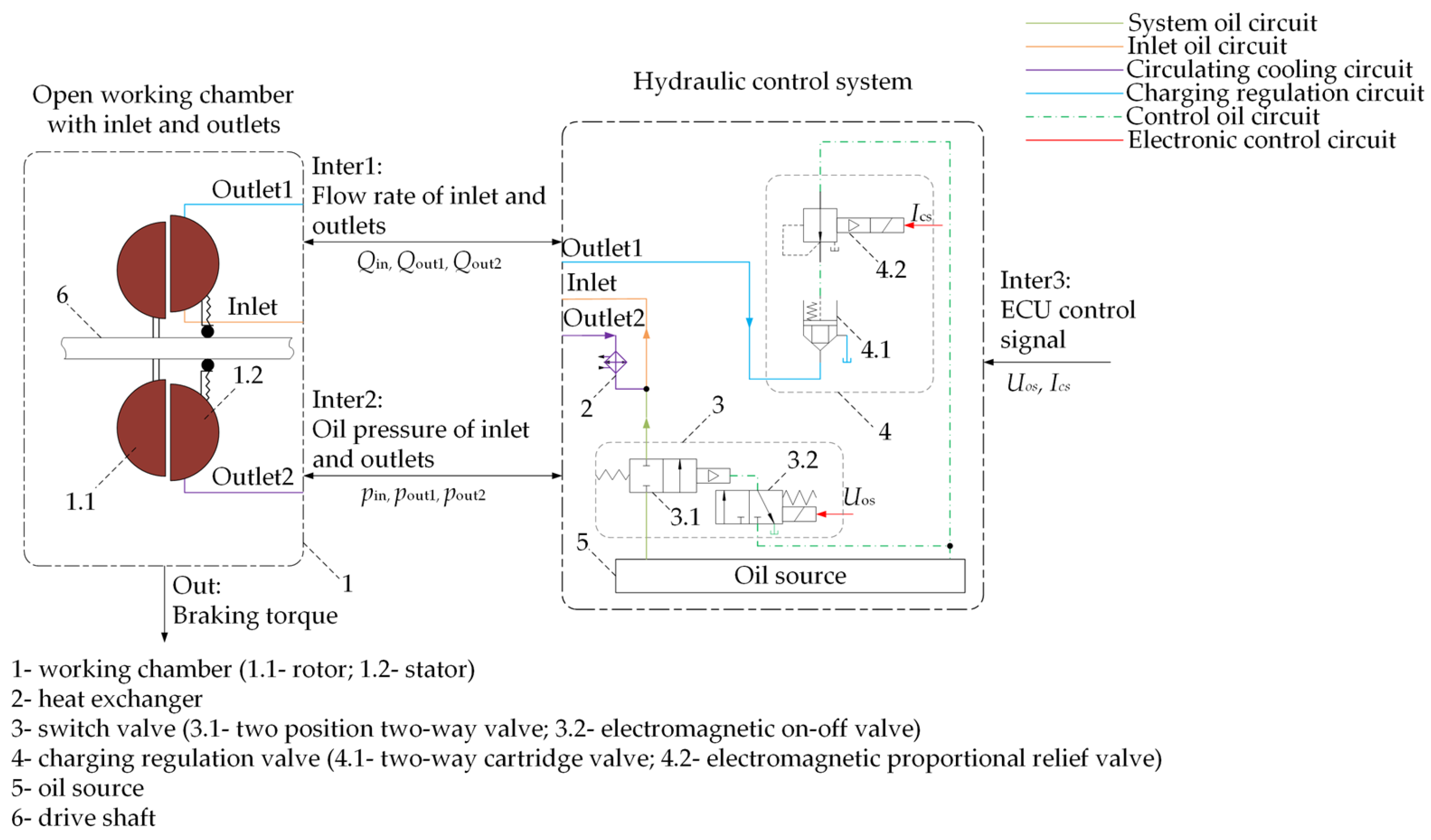
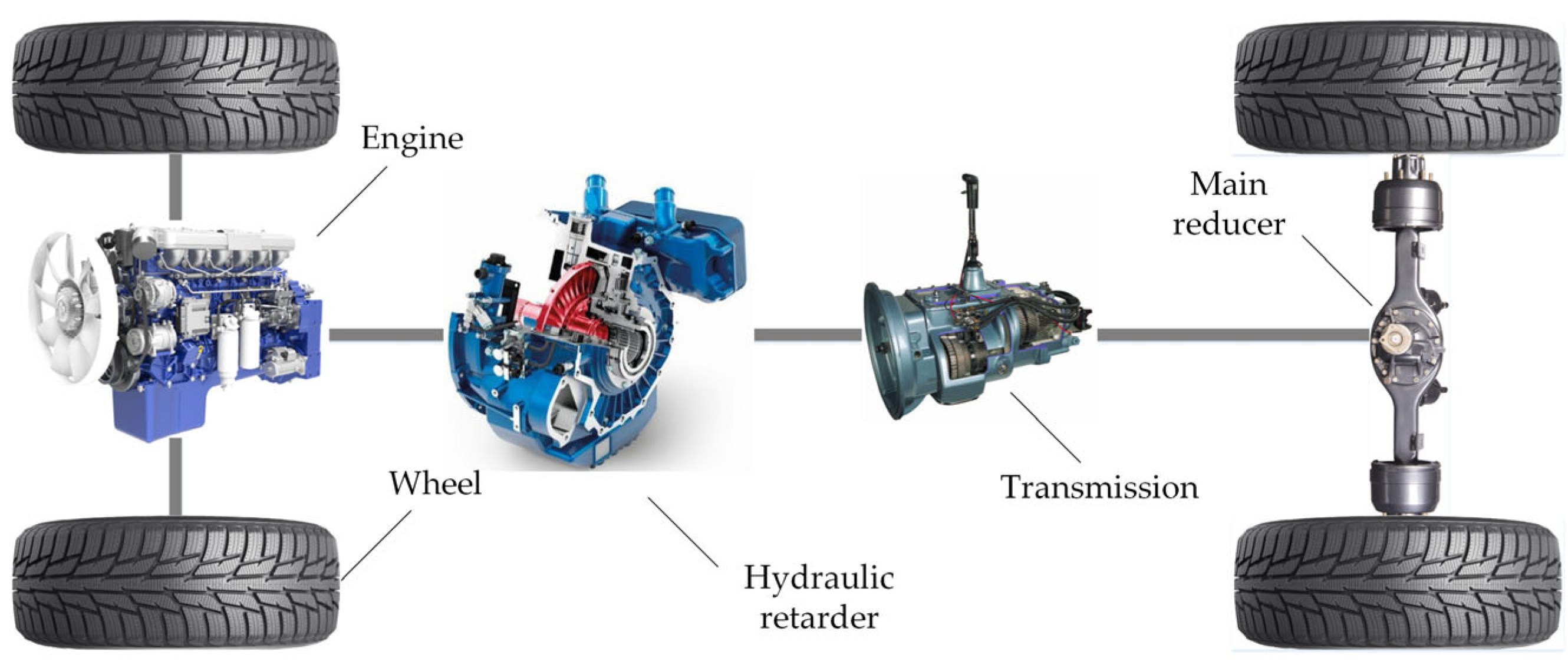
2.1. Hydraulic Retarder Model

Figure 1 shows the open working chamber and hydraulic control model. The input, output, and interaction parameters between the two models are defined in Figure 1 as well. The retarder working chamber is constituted by the rotor 1.1 and the stator 1.2 with blades; the rotor is connected to the output shaft, whereas the stator is fixed to a fixed component. When the retarder is operational, the system oil controlled by the switch valve 3 flows from the system oil circuit into the retarder working cavity between the rotor and stator. At this time, the rotor moves the hydraulic fluid in the working chamber. Meanwhile, the stator 1.2 is fixed, which will produce the reaction force. The rotor receives the reaction force to impede its rotation, which generates the braking torque to slow down the vehicle [8]. For the working chamber, oil discharged from outlet A will flow into the circulating cooling circuit, which could be cooled by the heat exchanger. Then, oil returns to the working chamber through the inlet oil circuit, thus completing the self-circulating cooling process. Additionally, oil outflowing from outlet B will enter the charging regulation circuit. The ECU transmits the control signal to the charging regulation valve 4, containing a two-way cartridge valve 4.1 and an electromagnetic proportional pressure relief valve 4.2, which adjusts the hydraulic retarder filling rate by changing the oil pressure of outlet B.

The hydraulic retarders can be divided into two types according to their installation positions: one is installed behind the engine, and the other is behind the transmission [26]. Compared with the installation behind the transmission, the hydraulic retarder installed behind the engine may cause power interruption and impact in the process of shifting gears when the vehicle is braking. However, hydraulic retarders in this installation position tend to have stronger low-speed braking performance, which can better satisfy the braking requirements of the vehicle traveling slowly downhill. In this study, the hydraulic retarder is installed behind the engine. Figure 2 shows the hydraulic retarder mounting position.

The amount of retarder braking torque is mainly dependent on the vehicle speed, the amount of working fluid, and other factors. Based on one-dimensional flow theory and the structural parameters of the hydraulic retarder, the braking torque of a fully oil-filled hydraulic retarder at a constant revolution could be estimated as follows [27]:

$$M_r=\lambda \rho n^2{D}^5$$

(1)

where $\lambda$ is the braking torque coefficient of the hydraulic retarder, the value of $\lambda$ in this paper is taken to be 0.001. $\rho$ (kg/m³) is the hydraulic retarder working oil density, the fluid of the retarder is commonly used mineral hydraulic oil, and the density of the fluid is set as 860 kg/m³. $n$ (rpm) is the hydraulic retarder rotor speed. $D$ (m) is the effective diameter of the retarder circuit; the value of $D$ in this paper is taken to be 0.293 m.

In the actual working process, when the hydraulic reducer is involved in braking, its internal state is usually in a partially filled state. Under this condition, the flow field inside the hydraulic reducer presents complex gas–liquid two-phase flow characteristics. Compared with the full-flooded condition, the braking performance prediction and calculation process in this partially-flooded condition has higher complexity, which is mainly reflected in the two-phase flow interactions, dynamic changes of the phase interface, and energy dissipation mechanisms. The literature [12] adopts the uniform density method and gas–liquid layering method to establish mathematical models for the braking performance of the hydraulic reducer under partially liquid-filled working conditions, and the comparative analysis of example calculations and experimental data shows that the uniform density method is simple and easy to carry out, while the calculation method of the gas–liquid layering method is relatively complex and theoretically more accurate, but its reasonableness still needs to be further verified through the partially liquid-filled braking performance test.

Using the uniform density method, the braking torque of the hydraulic retarder under a partially filled condition can be approximated and simplified as the product of the filling rate and the full-filled braking torque at this speed:

$$M_r=\lambda \rho n^2{D}^{5}q$$

(2)

where $q$ (%) is the filling rate of the working cavity.

When the hydraulic retarder is working, its working cavity can convert into the kinetic energy of the vehicle into the internal energy of the working fluid, embodied in the hydraulic retarder outlet of the high-temperature working fluid, and the high-temperature working fluid enters the radiator of the cooling system and then dissipates the heat. If the heat dissipation capacity of the cooling system is unable to dissipate all the heat generated by the hydraulic retarder, the overall temperature of the coolant will rise. When the temperature rises above the permissible value, the controller needs to reduce the braking power output of the hydraulic retarder to ensure the safety and stability of the cooling system. That is, the maximum braking power that the hydraulic retarder can continuously output and the corresponding braking torque should depend on the maximum cooling power that can be dissipated by the engine cooling system.

As previously demonstrated, the hydraulic retarder braking torque formula can be used to calculate the corresponding retarder braking power; its equation is as follows:

$$P_r={\displaystyle \frac{M_{r}n}{9549}}$$

(3)

where $M_r$ (N·m) is the hydraulic retarder braking torque when the retarder working cavity is partially filled with oil. $n$ (rpm) is the rotor speed of the hydraulic retarder.

When the working cavity of the hydraulic retarder is entirely filled with oil, the maximum braking power that the hydraulic retarder can generate at the present vehicle speed is expressed as follows:

$$P_{r\max }={\displaystyle \frac{\lambda \rho n^3{D}^5}{9549}}$$

(4)

When the vehicle needs a hydraulic retarder for deceleration braking in downhill driving, the driver starts the retarder, and the oil begins to flow into the working cavity, generating braking torque, which enters the deceleration braking stage of the vehicle downhill braking process, and the controller calculates the maximum braking power of the hydraulic retarder under the present speed and the filling rate to compare it with the maximum radiator cooling power, so as to fulfill the braking requirement of the entire vehicle downhill deceleration braking process under the premise of ensuring the vehicle’s radiator system safety. The controller will calculate the maximum braking power of the retarder at the present speed with the filling rate and compare it to the maximum cooling power of the radiator to achieve the braking requirement of the downhill deceleration braking process while ensuring the vehicle’s cooling system safety. When the vehicle has decelerated to the vicinity of the driver’s desired target speed, the driver opens the constant speed switch, at which time the braking process enters the constant-speed braking stage, and the electronic control unit records the present vehicle speed as the target speed. The error signal between the present speed and the target speed is input to the constant speed controller. The controller changes the braking torque of the retarder by changing the retarder filling rate to achieve the goal of driving downhill at a constant speed. The vehicle downhill constant-speed control flowchart is shown in Figure 3, where $P_r$ is the braking power of the retarder working cavity partially filled with oil, $P_{r\max }$ is the maximum braking power of the retarder, and $P_b$ is the braking power output of the retarder. $P_c$ is the heat dissipated power provided by the cooler of the cooling circulation system. The maximum heat dissipation power that can be provided by the cooler of the cooling circulation system in this research is 500 kW.

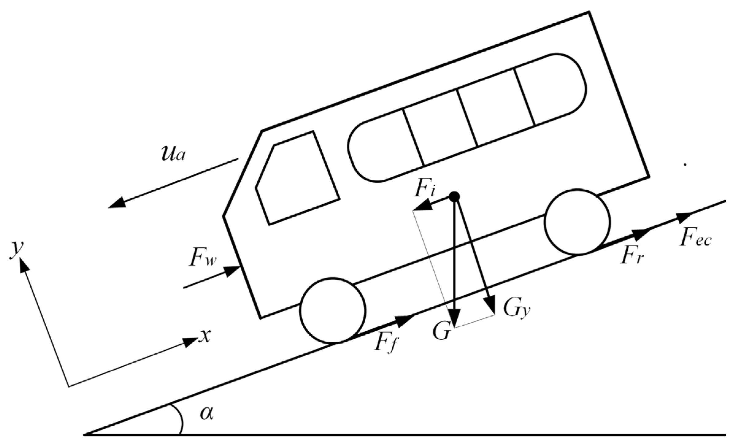
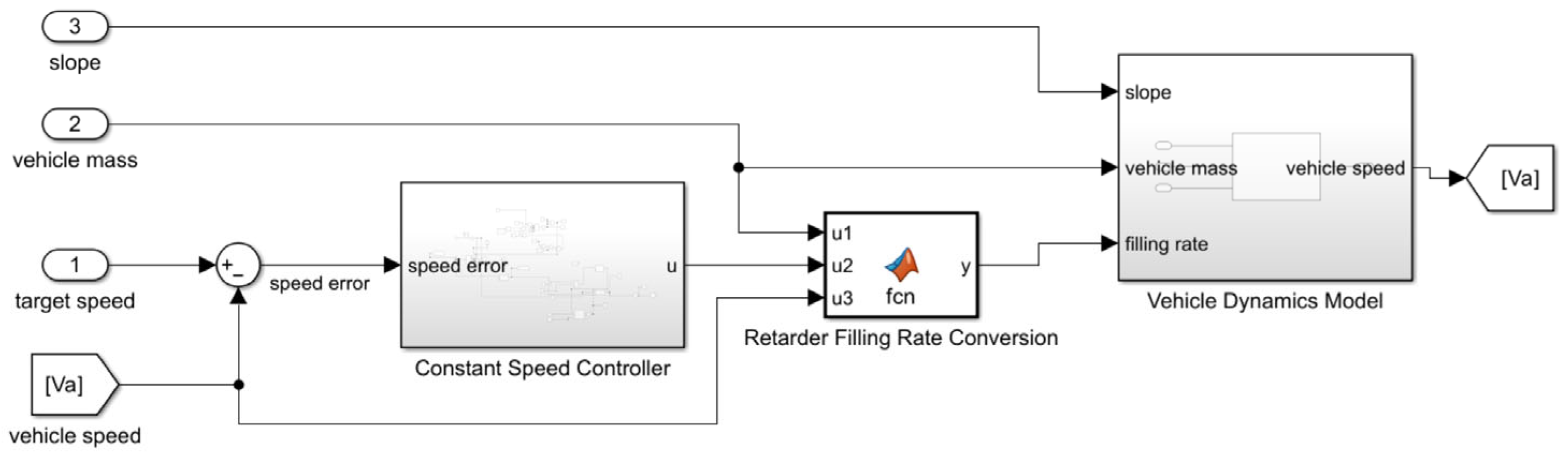
2.2. Vehicle Dynamics Model

The downhill braking force analysis of heavy vehicles with hydraulic retarders is presented in Figure 4. Let the heavy vehicles along the slope of the ramp be straight downhill travelling; downhill travelling ramp length is long enough; in the process of travelling, the vehicle wheels are pure rolling, the main brake and accelerator pedal are not working, and the hydraulic retarder is in the working state. According to Newton’s Second Law of Motion, the establishment of the vehicle downhill driving dynamics equation for Equation (4).

$$m{\displaystyle \frac{dv}{dt}}=F_i-F_r-F_w-F_f-F_{ec}$$

(5)

where $m$ (kg) is the mass of vehicle, $v$ (km/h) is the current vehicle velocity, $F_i$ (N) is the gravity fraction in direction of vehicle travel along the ramp, $F_r$ (N) is the braking force produced by the hydraulic retarder on the wheels, $F_w$ (N) is the air resistance, $F_f$ (N) is the rolling resistance, $F_{ec}$ (N) is the engine braking force.

The gravity fraction in direction of vehicle travel along the ramp is expressed as follows:

$$F_i=G\sin \alpha$$

(6)

where $G$ (N) is the gravity of the vehicle, $\alpha$ (%) is the slope of the road.

According to China’s Expressway Design Specification, the mountain ridge heavy slope area of the expressway is 5%, and the maximum slope of the plain micro-hill area is 3%; the first-class automobile special highway mountain ridge heavy slope area is 6%, and the maximum slope of the plain micro-hill area is 4%; the general four-level highway mountain ridge heavy slope area is 9%, and the plain micro-hill area is 5%. Therefore, the slope of the general roads can be obtained as follows:

$$\sin \alpha \approx \tan \alpha =i,\cos \alpha =1$$

(7)

The force of gravity can be written as follows:

$$F_i=G\sin \alpha \approx Gi$$

(8)

$F_r$ is the braking force created by the hydraulic retarder on the wheels; from the foregoing part of the hydraulic retarder braking torque formula, the braking force expression may be determined as follows:

$$F_r={\displaystyle \frac{M_r{\eta }_t{i}_0{i}_g}{r}}={\displaystyle \frac{\lambda \rho {\eta }_t{n}^2{D}^5{i}_0{i}_{g}q}{r}}={\displaystyle \frac{\lambda \rho {\eta }_t{v}^2{D}^5{i_0}^3{i_g}^{3}q}{{\left(0.377\right)}^2{r}^3}}$$

(9)

where $i_0$ is the gear ratio of the main reducer, $i_g$ is the gear ratio of the transmission, ${\eta }_t$(%) is the vehicle mechanical transmission efficiency, $r$ (m) is the wheel radius.

The air resistance of the vehicle travelling downhill can be expressed as follows:

$$F_w=C_{D}A{v}^2/21.15$$

(10)

where $C_D$ is the aerodynamic resistance coefficient, $A$(m²) is the windward area.

The rolling resistance is expressed as follows:

$$F_f=Gf\cos \alpha$$

(11)

where $f$ is the rolling resistance coefficient equal to $0.0076+0.000056u_a$, $u_a$ is the present vehicle velocity.

Vehicles are prohibited from coasting in neutral when travelling long distances downhill. Therefore, when descending a hill, the clutch must remain engaged with the vehicle driveline, as the vehicle is not disengaged from the engine. During this process, the engine’s compression stroke, influenced by compression resistance, internal friction, and intake and exhaust resistance, generates a certain amount of braking force on the wheels. The mathematical formula for the braking torque of the motor is expressed as follows:

$$M_{ec}={\displaystyle \frac{1000p_m{V}_h}{\pi \tau }}$$

(12)

where $V_h$ (m²) is the working volume of the engine cylinders, $\tau$ is the number of engine strokes, $p_m$ (Pa) is the average mechanical loss pressure of the engine.

The average mechanical loss pressure of the engine is influenced by various factors, including the engine’s crankshaft, pistons, and other mechanical components. Additionally, it is affected by the engine’s load, speed, and numerous other operational parameters. In practice, an empirical formula that is often employed to determine the engine’s average mechanical loss pressure is as follows:

$$p_m=3.5864-0.5283C_m+0.2728C_m^2$$

(13)

where $C_m$ is the piston movement average speed equal to ${\displaystyle \frac{sn}{30}}$, $s$ is the piston stroke, $n$ is the engine speed.

Given that the engine braking torque must be transmitted through the transmission to the brake wheel, the actual role of the engine braking torque on the brake wheel should be multiplied by the transmission and the main gear ratio, in accordance with the above formula. Consequently, the engine braking force can be expressed as follows:

$$F_{ec}={\displaystyle \frac{1000i{p}_m{V}_h{\eta }_t}{\pi \tau }}$$

(14)

where $i$ is the total vehicle gear ratio, ${\eta }_t$ is the vehicle mechanical transmission efficiency.

Upon substituting the aforementioned equation into Equation (4), the dynamic equation of the vehicle driving downhill is established as Equation (14):

$$\dot{v}=g\left(i-f\right)-{\displaystyle \frac{C_{D}A{v}^2}{21.15m}}-{\displaystyle \frac{\lambda \rho {\eta }_t{v}^2{D}^5{i_0}^3{i_g}^{3}q}{{\left(0.377\right)}^2{r}^{3}m}}-{\displaystyle \frac{1000i{p}_m{V}_h{\eta }_t}{\pi \tau m}}$$

(15)

3. Controller Design

Due to the high degree of nonlinearity and uncertainty of the vehicle system, this study chooses to use the sliding mode control idea to design the controller and takes the difference between the target speed and the actual speed as the controller input and takes the hydraulic retarder target filling rate as the controller output.

We define the nonlinear dynamics of the system $f(v)$ and the controller input $u$ as follows:

$$f(v)=g\left(i-f\right)-{\displaystyle \frac{C_{D}A{v}^2}{21.15m}}-{\displaystyle \frac{1000i{p}_m{V}_h{\eta }_t}{\pi \tau m}}$$

(16)

$$u=-{\displaystyle \frac{\lambda \rho {\eta }_t{v}^2{D}^5{i_0}^3{i_g}^{3}q}{{\left(0.377\right)}^2{r}^{3}m}}$$

(17)

Then Equation (14) can be rewritten as follows:

$$\dot{v}=g\left(i-f\right)-{\displaystyle \frac{C_{D}A{v}^2}{21.15m}}-{\displaystyle \frac{\lambda \rho {\eta }_t{v}^2{D}^5{i_0}^3{i_g}^{3}q}{{\left(0.377\right)}^2{r}^{3}m}}-{\displaystyle \frac{1000i{p}_m{V}_h{\eta }_t}{\pi \tau m}}=f\left(v\right)+u$$

(18)

Lemma 1.

For a controlled system:

$$\dot{v}=f\left(v\right)+u$$

(19)

The controller input $u={\dot{v}}_d+ke(t)+u_{aux}$ can control the system to a given target vehicle speed $v_d$, where $u_{aux}$ is the controller auxiliary term equal to $\rho (v){\displaystyle \frac{\left|\left.e(t)\right|\right.}{e(t)}}$, $k>0$, $\rho (v)>\left.\left|f(v)\right.\right|$, $e(t)=v_d-v$, where $v_d$ is the target vehicle speed [28]. In this research, the target vehicle speed is unchanged, which gives ${\dot{v}}_d=0$.

The stability of sliding mode control is usually analyzed based on the Lyapunov method, where the stability of the control system is demonstrated by constructing a Lyapunov function, constructing the Lyapunov function as follows:

$$V_{(e(t))}={\displaystyle \frac{1}{2}}e{(t)}^2$$

(20)

Differentiating Equation (19) gives

$$\begin{array}{l}{\dot{V}}_{(e(t))}=e(t)\dot{e}(t)=e(t)({\dot{v}}_d-\dot{v})=e(t)({\dot{v}}_d-f(v)-u)\\ =-ke{(t)}^2-e(t)f(v)-e(t)\rho (v){\displaystyle \frac{\left|e(t)\right|}{e(t)}}\\ =-ke{(t)}^2-e(t)f(v)-\rho (v)\left|e(t)\right|\\ \le -ke{(t)}^2+\left|e(t)\right|\left|f(v)\right|-\rho (v)\left|e(t)\right|\\ \le -ke{(t)}^2=-2k{V}_{(e(t))}\end{array}$$

(21)

Introduce a slack variable $s(t)>0$ to transform inequality ${\dot{V}}_{(e(t))}\le -2k{V}_{(e(t))}$ into an equation:

$${\dot{V}}_{(e(t))}+2k{V}_{(e(t))}+s(t)=0$$

(22)

This is a first-order linear non-homogeneous equation, and its general solution is as follows:

$$V_{(e(t))}=V_{(e(0))}{e}^{-2kt}-e^{-2kt}{\displaystyle {\int }_0^t{e}^{2k\tau }}s(\tau )d\tau$$

(23)

Since for $s(t)>0$,$e^{2k\tau }>0$,$e^{-2kt}>0$, we obtain inequality $V_{(e(t))}\le V_{(e(0))}{e}^{-2kt}$ as follows:

$$e{(t)}^2\le e{(0)}^2{e}^{-2kt}$$

(24)

Taking the square root of both sides of the inequality provides $\left|e(t)\right|\le \left|e(0)\right|e^{-kt}$, which is a kind of exponential asymptotic stability, resulting in the speed target error $e$ being asymptotically stable.

From the above proof, it can be concluded that the system is asymptotically stable, and the system’s input is as follows:

$$u=-{\displaystyle \frac{\lambda \rho {\eta }_t{v}^2{D}^5{i_0}^3{i_g}^{3}q}{{\left(0.377\right)}^2{r}^{3}m}}={\dot{v}}_d+ke(t)+\rho (v){\displaystyle \frac{\left|e(t)\right|}{e(t)}}=ke(t)+\rho (v){\displaystyle \frac{\left|e(t)\right|}{e(t)}}$$

(25)

The equation for the hydraulic retarder filling rate is expressed as follows:

$$q={\displaystyle \frac{ke(t)+\rho (v)\frac{\left|e(t)\right|}{e(t)}}{-\frac{\lambda \rho {\eta }_t{v}^2{D}^5{i_0}^3{i_g}^3}{{\left(0.377\right)}^2{r}^{3}m}}}$$

(26)

Considering that the input in the above control system contains ${\displaystyle \frac{\left|e(t)\right|}{e(t)}}$, which will switch back and forth from 1 to −1, causing rapid switching of the control input, which may result in high-frequency chattering, in order to suppress the sliding mode chattering, this paper presents a design of the controller based on the sliding mode control, utilizing saturation function and high-frequency control concept.

(1)

The use of saturation function to suppress sliding mode chattering refers to the use of saturation function to replace the sign function in the control system and the use of saturation function continuity to achieve the purpose of weakening the sliding mode control system chattering [23]. The saturation function employed in this study is expressed as follows:

$$sat(e(t))=\left\{\begin{array}{ll}1,\hfill & e(t)>\Delta \hfill \\ 1/\Delta ,\hfill & \left|e(t)\right|\le \Delta \hfill \\ -1,\hfill & e(t)<\Delta \hfill \end{array}\right.$$

(27)

where $\Delta$ is the boundary layer.

Then the sliding mode controller input can be further expressed as follows:

$$u=ke(t)+\rho (v){\displaystyle \frac{\left|e(t)\right|}{e(t)}}=ke(t)+\rho (v)sat(e(t))$$

(28)

The equation for the hydraulic retarder filling rate is expressed as follows:

$$q={\displaystyle \frac{ke(t)+\rho (v)sat(e(t))}{-\frac{\lambda \rho {\eta }_t{v}^2{D}^5{i_0}^3{i_g}^3}{{\left(0.377\right)}^2{r}^{3}m}}}$$

(29)

(2)

The high-frequency robust controller is based on the sliding mode controller for the optimization of the upper and lower limits of the positive and negative value switching of the controller, by adding a real number $\epsilon$ greater than 0 to the denominator of the auxiliary term of the controller, it makes the input switching of the high-frequency robust controller smoother and reduces the degree of switching intensity.

Lemma 2.

For a controlled system:

$$\dot{v}=f\left(v\right)+u$$

(30)

The controller input $u$ can control the system to a given target vehicle speed $v_d$, where $u={\dot{v}}_d+ke+{\displaystyle \frac{\rho {(v)}^{2}e(t)}{\rho (v)\left|e(t)\right|+\epsilon }}$, $k>0$, $\epsilon >0$, considering the model accuracy error and the sensor measurement error in practice, $\rho (v)$ is usually taken as $\rho (v)>\left.\left|f(v)\right.\right|$, $e(t)=v_d-v$, $v_d$ is the target vehicle speed [28]. In this research, the target vehicle speed is unchanged, which gives ${\dot{v}}_d=0$.

The stablity of the high-frequency robust control system is demonstrated below by constructing the Lyapunov function as follows:

$$V_{(e(t))}={\displaystyle \frac{1}{2}}e{(t)}^2$$

(31)

Differentiating Equation (30) gives

$$\begin{array}{l}{\dot{V}}_{(e(t))}=e(t)\dot{e}(t)=e(t)(-f(v)-ke(t)-{\displaystyle \frac{\rho {(v)}^{2}e(t)}{\rho (v)\left|e(t)\right|+\epsilon }})\\ =-ke{(t)}^2-f(v)e(t)-e(t){\displaystyle \frac{\rho {(v)}^{2}e(t)}{\rho (v)\left|e(t)\right|+\epsilon }}\\ \le -ke{(t)}^2+\rho (v)\left|e(t)\right|-e(t){\displaystyle \frac{\rho {(v)}^{2}e(t)}{\rho (v)\left|e(t)\right|+\epsilon }}\\ =-ke{(t)}^2+{\displaystyle \frac{\rho {(v)}^2{\left|e(t)\right|}^2+\rho (v)\left|e(t)\right|\epsilon -\rho {(v)}^2{\left|e(t)\right|}^2}{\rho (v)\left|e(t)\right|+\epsilon }}\\ =-ke{(t)}^2+\epsilon ({\displaystyle \frac{\rho (v)\left|e(t)\right|}{\rho (v)\left|e(t)\right|+\epsilon }})\le -ke{(t)}^2+\epsilon \end{array}$$

(32)

Introduce a slack variable $s(t)>0$ to transform inequality ${\dot{V}}_{(e(t))}\le -2k{V}_{(e(t))}+\epsilon$ into an equation as follows:

$$V_{(e(t))}=V_{(e(0))}{e}^{-2kt}-e^{-2kt}{\displaystyle {\int }_0^t{e}^{2k\tau }}s(\tau )d\tau +\epsilon e^{-2kt}{\displaystyle {\int }_0^t{e}^{2k\tau }}d\tau$$

(33)

This is a first-order linear non-homogeneous equation, and its general solution is as follows:

$$V_{(e(t))}=V_{(e(0))}{e}^{-2kt}-e^{-2kt}{\displaystyle {\int }_0^t{e}^{2k\tau }}s(\tau )d\tau +\epsilon e^{-2kt}{\displaystyle {\int }_0^t{e}^{2k\tau }}d\tau$$

(34)

where $s(t)>0$, $e^{-2kt}>0$, $V(e(t))={\displaystyle \frac{1}{2}}e{(t)}^2$.

Integrating over $\epsilon e^{-2kt}{\displaystyle {\int }_0^t{e}^{2k\tau }}d\tau$, the preceding equation is simplified as follows:

$${\displaystyle \frac{1}{2}}e{(t)}^2\le {\displaystyle \frac{1}{2}}e(0)e^{-2kt}+{\displaystyle \frac{\epsilon }{2k}}\left[1-e^{-2kt}\right]$$

(35)

Taking the square root on both sides of the inequality:

$$\left|e(t)\right|\le \sqrt{\left|e(0)\right|e^{-2kt}+{\displaystyle \frac{\epsilon }{k}}-{\displaystyle \frac{\epsilon }{k}}{e}^{-2kt}}$$

(36)

When $t\to \infty$, $\left|e(t)\right|\le \sqrt{{\displaystyle \frac{\epsilon }{k}}}$. This is a globally consistent and bounded conclusion, and the suitable $\epsilon >0$ can be selected to stabilize the system asymptotically.

The equation for the hydraulic retarder filling rate with a high-frequency controller is expressed as follows:

$$q={\displaystyle \frac{ke+\frac{\rho {(v)}^{2}e(t)}{\rho (v)\left|e(t)\right|+\epsilon }}{-\frac{\lambda \rho {\eta }_t{v}^2{D}^5{i_0}^3{i_g}^3}{{\left(0.377\right)}^2{r}^{3}m}}}$$

(37)

4. Simulation Results and Analysis

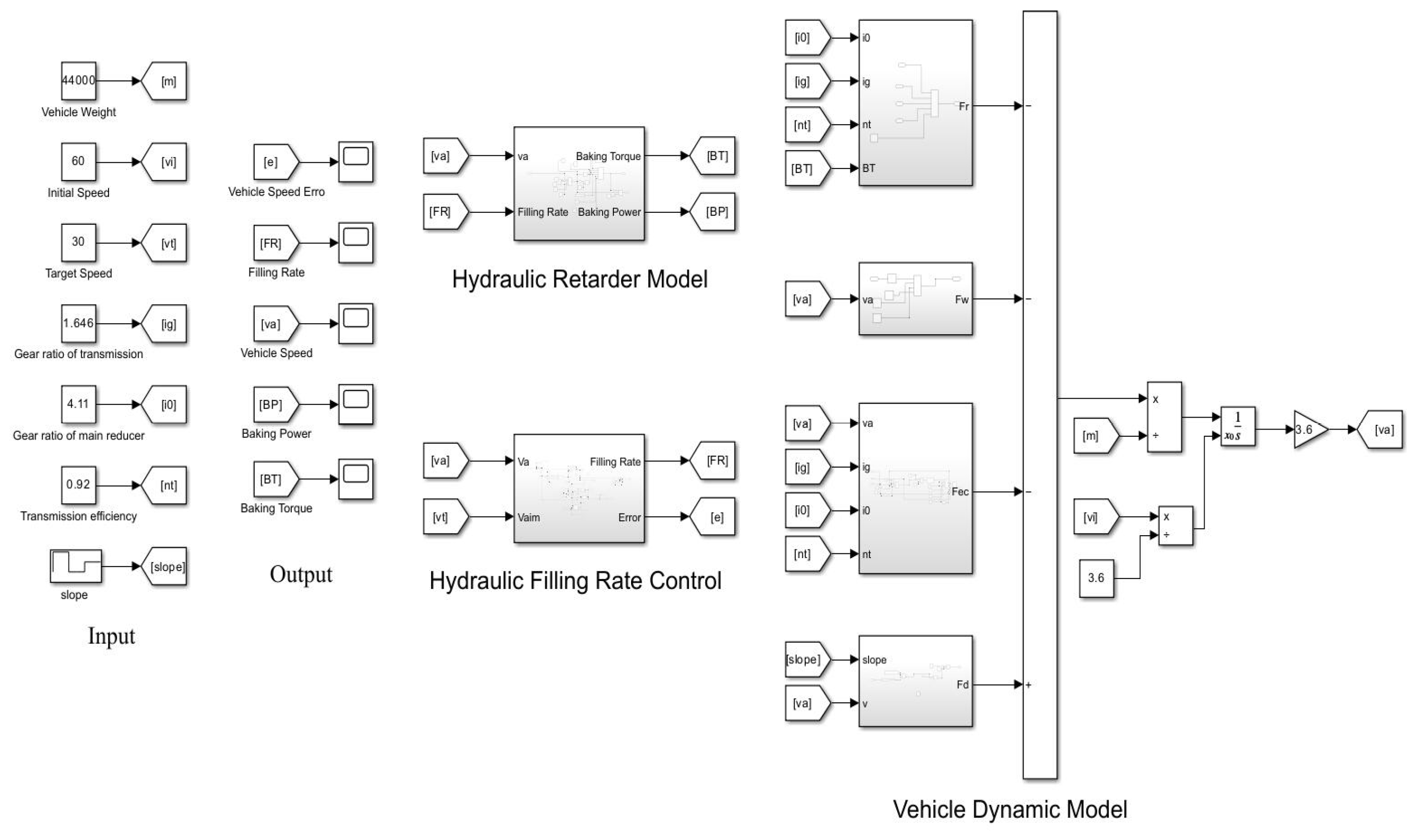
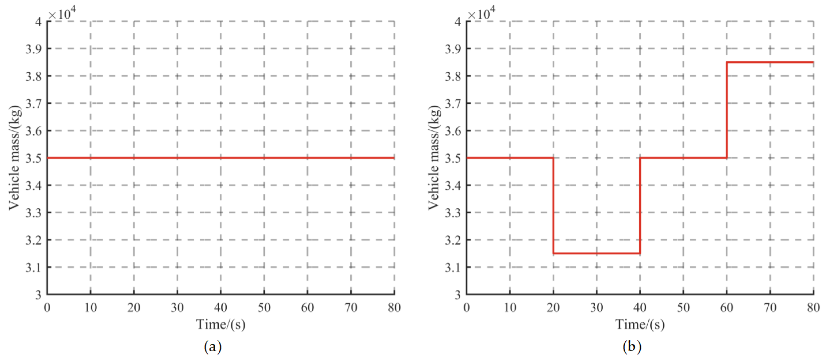
4.1. Heavy-Duty Vehicle Simulation Conditions

According to the vehicle downhill dynamic equations established by Equation (14), the constant speed control strategy during continuous braking is simulated and analyzed in the MATLAB/Simulink environment, and the overall simulation model of heavy-duty vehicle downhill braking is established as shown in Figure 5. Figure 6 shows the constant speed control logic for the vehicle travelling downhill. The controller control structure schematic is shown in Figure 7. In order to test the viability of the controller created in this work, simulation experiments were carried out utilizing the sliding mode control algorithm and fuzzy control algorithm models [Appendix A] under varied operating conditions.

Assuming the vehicle is traveling downhill in third gear, with a speed of 60 km/h, the vehicle descends without involving mechanical brakes, travels in a straight line on a flat road with adequate grip, and the wheels do not lock or skid. The hydraulic retarder filling delay time of 0.1 s is considered in the simulation. The simulation time was set to 80 s, and the simulation step was set to 0.1 s. The main simulation parameters for the system are detailed in

Table 1. Main parameters of simulation model.

Parameter	Value
Initial vehicle velocity	60 km/h
Target vehicle velocity	30 km/h
Aerodynamic resistance coefficient	0.65
Windward area	5 m2
Density of fluid medium	860 kg/m3
Gear ratio of transmission	1.646
Gear ratio of main reducer	4.111
Wheel radius	0.554 m
Simulation step	0.1 s

. To test the performance of the control strategy, a fixed vehicle mass M1 and a varying vehicle mass M2 were set to complete the simulation, as shown in Figure 8. In addition, three road gradient conditions, S1, S2, and S3, were designed to verify the performance of the controller, as shown in Figure 9.

This paper compares the performance of different hydraulic retarder filling rate controllers by varying the vehicle payload and the gradient conditions of the road during the long downhill drive. As shown in

Table 2. Simulation conditions.

	Mass	M1	M2
Slope
S1		C1	C2
S2		\	C3

, three different simulation conditions, C1, C2, and C3, are designed in this paper.

In Section 3 high-frequency controller design, the values of the two hyperparameters, $k$ and $\epsilon$, will have a great impact on the high-frequency controller speed tracking performance and control outputs. In this paper, three different combinations of $k$ and $\epsilon$ are selected, respectively, and simulation experiments are carried out under C2 conditions, and the control performance of high-frequency controllers with different parameter combinations is compared and analyzed, and the simulation results are shown in Figure 9. The RMSE (Root Mean Square Error) and Max (Maximum Absolute Speed Error) of the speeds are shown in

Table 3. Comparison of speed error results for different control parameters.

	RMSE	Max
$k$ = 0.1, $\epsilon$ = 0.01	0.145	0.165
$k$ = 1, $\epsilon$ = 0.01	0.0652	0.0749
$k$ = 1, $\epsilon$ = 0.1	0.182	0.194

.

Figure 10a illustrates that an increase in the value of $k$ within the controller enhances the system’s response speed, hence accelerating the regulation of the vehicle’s speed. Table 3 shows that when the value of $k$ is fixed, the value of $\epsilon$ is directly proportional to the RMSE and Max of the vehicle speed. This indicates that the smaller the value of $\epsilon$, the better the speed tracking performance of the controller. By analysing Figure 10b, it can be seen that as the value of $\epsilon$ diminishes, the oscillation amplitude of the hydraulic retarder filling rate at the controller output increases, and an excessively low value of $\epsilon$ will result in high-frequency chatter in the control input. Considering the vehicle speed tracking performance requirements and the smoothness of the controller output, the control parameters of the high-frequency controller designed in this paper are $k$ = 1 and $\epsilon$ = 0.01.

4.2. Simulation Results

The RMSE and Max of the speeds of the three controllers under different vehicle loads and road gradients are shown in

Table 4. Comparison of controller speed error results.

	C1 (km/h)		C2 (km/h)		C3 (km/h)
Fuzzy control	RMSE	Max	RMSE	Max	RMSE	Max
	0.0176	0.0195	0.0729	0.113	0.184	0.370
High-frequency	RMSE	Max	RMSE	Max	RMSE	Max
	0.0841	0.0842	0.0652	0.0679	0.0683	0.122
Sliding mode	RMSE	Max	RMSE	Max	RMSE	Max
	0.0704	0.0716	0.0703	0.0790	0.0674	0.0905

. Figure 10, Figure 11 and Figure 12 show the simulation results of different controllers for long downhill slopes of heavy vehicles under three simulation conditions.

Analyzing the data in Table 4, it can be observed that the fuzzy controller has the best speed tracking performance with the RMSE of speed of 0.01759 and the maximum absolute error of speed of 0.0195 in the C1 simulation scenario. However, under the C3 simulation situation, the fuzzy controller has a huge gap in speed tracking performance compared to the other two controllers. The difference in speed tracking performance between the high-frequency controller and the sliding mode controller is not substantial. In the C2 situation, the RMSE of the high-frequency controller is 7.2% less than that of the sliding-mode controller, and the highest absolute error of the speed is 14.1% smaller than that of the sliding-mode controller. The sliding mode controller, on the other hand, shows the best speed tracking performance in the C3 condition, where the RMSE of the speed of the sliding mode controller is 1.4% less than that of the high-frequency controller, and the maximum absolute error of the speed is 25.8% less than that of the high-frequency controller.

Figure 11 illustrates the control effects of the three controllers under constant vehicle mass and fixed road gradient conditions. Figure 11a–d illustrate the vehicle speed, retarder filling rate, vehicle speed error, and retarder braking power, respectively. Upon activation of the retarder, the vehicle’s speed diminishes to approximately the target velocity within 15 s. The saturation function of the sliding mode controller, high-frequency controller, and fuzzy controller can swiftly and precisely determine the necessary retarder filling rate under current operating conditions, thereby satisfying the requirements for the vehicle’s slow downhill traveling. The fuzzy controller exhibits the highest control accuracy with the minimal speed error; nevertheless, it requires the longest duration, approximately 20.1 s, to approach the stable value. As the vehicle speed approaches the target speed, the control output (hydraulic retarder filling rate) of the sliding-mode controller with a saturation function exhibits pronounced chatter, accompanied by minor fluctuations in the high-frequency controller, whereas the fuzzy controller demonstrates superior output smoothing.

The simulation results considering the change in vehicle mass are shown in Figure 12a,b. The root-mean-square of the speed errors for the three controllers, under varying vehicle mass and specific slope conditions, exhibits minimal variation, indicating commendable speed tracking performance. The sliding mode controller with saturation function and high-frequency controller has smaller speed fluctuation when the vehicle mass changes, and the maximum absolute speed error is not more than 0.079 km/h. The fuzzy controller has a maximum absolute speed error of 0.113 km/h, and the speed variation is rather considerable. At the same time, when the vehicle mass changes, although the sliding mode controller can achieve rapid and stable regulation of vehicle speed, its control output of the hydraulic retarder filling rate signal will appear to have obvious chattering, which makes it difficult to adjust the filling rate of the hydraulic retarder in reality. The reaction time of the fuzzy controller is slow, and it normally takes about 2 s to output the appropriate retarder filling rate to stabilize the vehicle speed.

Figure 13a,b show the simulation results of the three controllers for the C3 condition. The root-mean-square error of the vehicle speed of the fuzzy controller under the C3 condition is 0.184 km/h, and the maximum absolute error is 0.37 km/h. Compared with the other two controllers, the fuzzy controller has a larger fluctuation of the vehicle speed, and the speed tracking performance is poor. In terms of controller control output, the retarder filling rate signal output from the high-frequency controller shows the best smoothing when the vehicle mass changes in steps and fluctuates only for a short period of time after the mass has changed. Sliding mode controllers with saturation functions exhibit high-frequency chatter. The retarder filling rate signal from the fuzzy controller shows poor smoothing.

Figure 11, Figure 12 and Figure 13 show that while the vehicle descends at its initial speed, the hydraulic retarder performs a dynamic filling process for about 1 s, and the vehicle’s speed gradually increases. After the first filling process concludes, as the vehicle’s speed is rather high at this time, the braking power of the hydraulic retarder will be limited by the cooling power of the radiator, remaining at a constant value of 500 kW, and the volume of working fluid in the working cavity of the retarder increases with the slowing down of the vehicle’s speed until the working cavity is full of the working fluid, while the hydraulic retarder filling rate achieves the maximum value. At around 20 s, the vehicle speed decreases to near the target speed, and the speed controller begins to operate. It calculates the required hydraulic retarder filling rate under the present working conditions based on the speed error or speed error rate, allowing the vehicle to continue descending at the target speed. The braking power output of the hydraulic retarder does not exceed the maximum cooling power of the radiator in the cooling system during the whole process.

In conclusion, when a vehicle with constant mass is traveling downhill at a set gradient of 6%, all three controllers can effectively meet the requirement of maintaining a constant speed during downhill travel, with the fuzzy controller showing stronger speed tracking performance and smoother control output than the other two controllers. However, when the mass of the vehicle or the gradient of the road changes, which is a common phenomenon for heavy vehicles travelling downhill for a long period of time, the sliding mode controller with saturation function has good speed tracking performance, but its control output of the retarder filling rate signal sometimes produces violent jitter, which makes it very difficult to regulate the retarder filling rate in the practical work. The fuzzy controller shows poor robustness when the vehicle mass and road gradient change at the same time; when the speed fluctuation is large, the speed tracking performance is poor. The high-frequency controller shows the best control performance, which is reflected in the better speed tracking performance and the smoothest control output.

5. Conclusions

For the constant-speed braking control of the hydraulic retarder when the vehicle is travelling downhill for a long period of time, this research proposes a constant speed control strategy based on sliding mode control theory, establishes the vehicle dynamics model and the constant speed control model of the hydraulic retarder under the MATLAB/Simulink environment, and carries out simulation tests, which verify the control effect of the controller. At the same time, the controller designed in this research is simulated and compared with the fuzzy controller. The subsequent conclusions are drawn from the simulation research conducted:

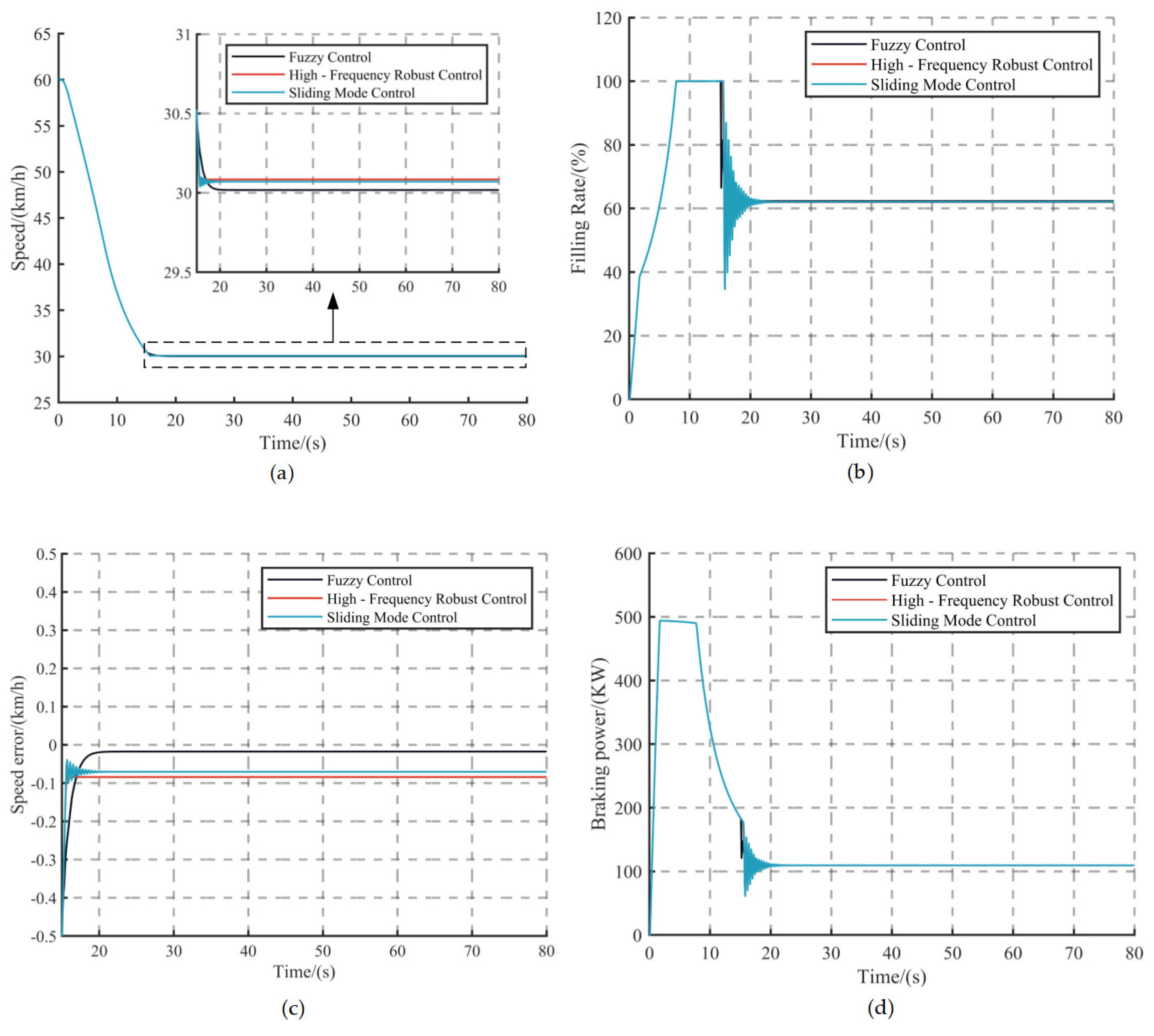
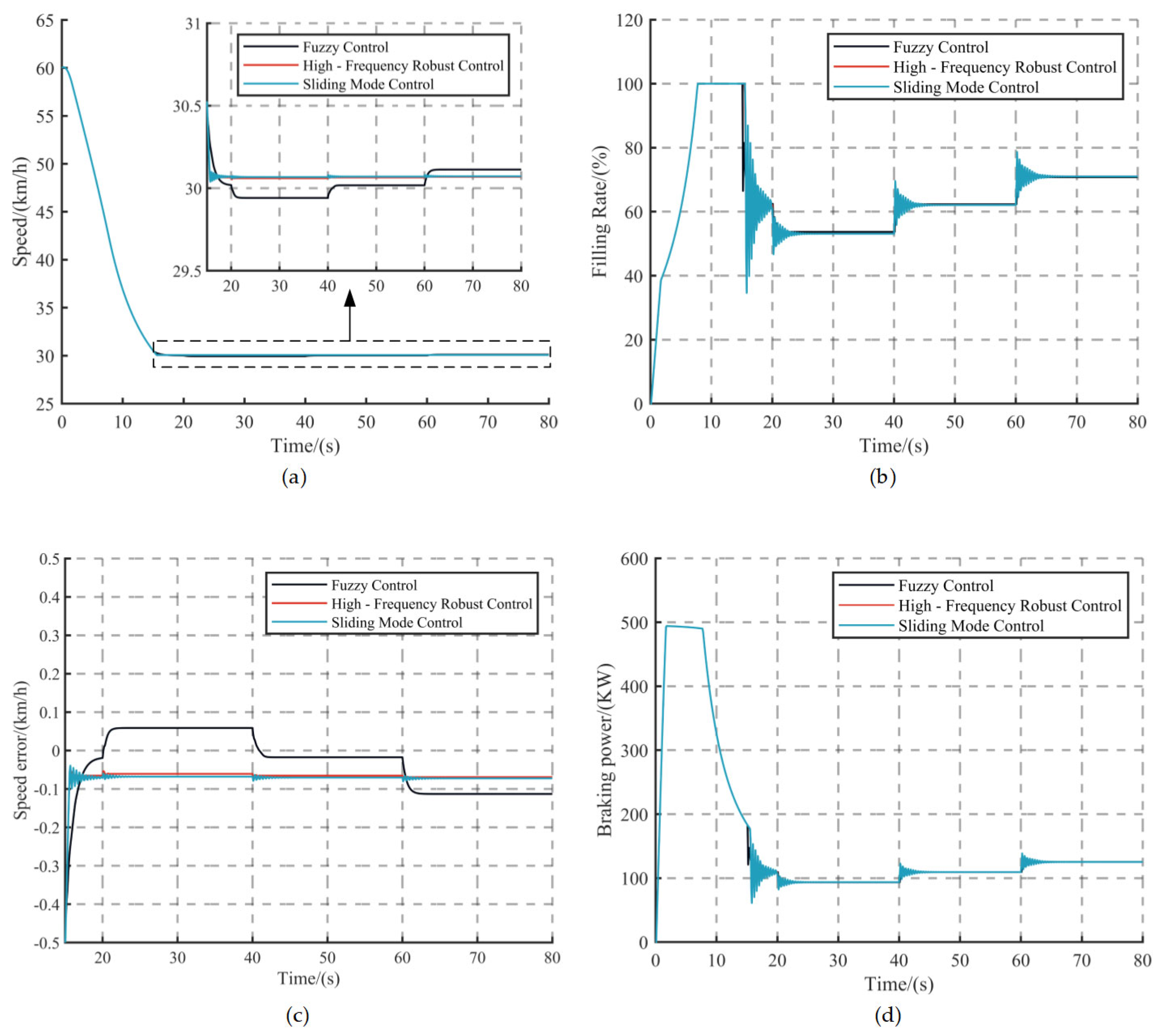
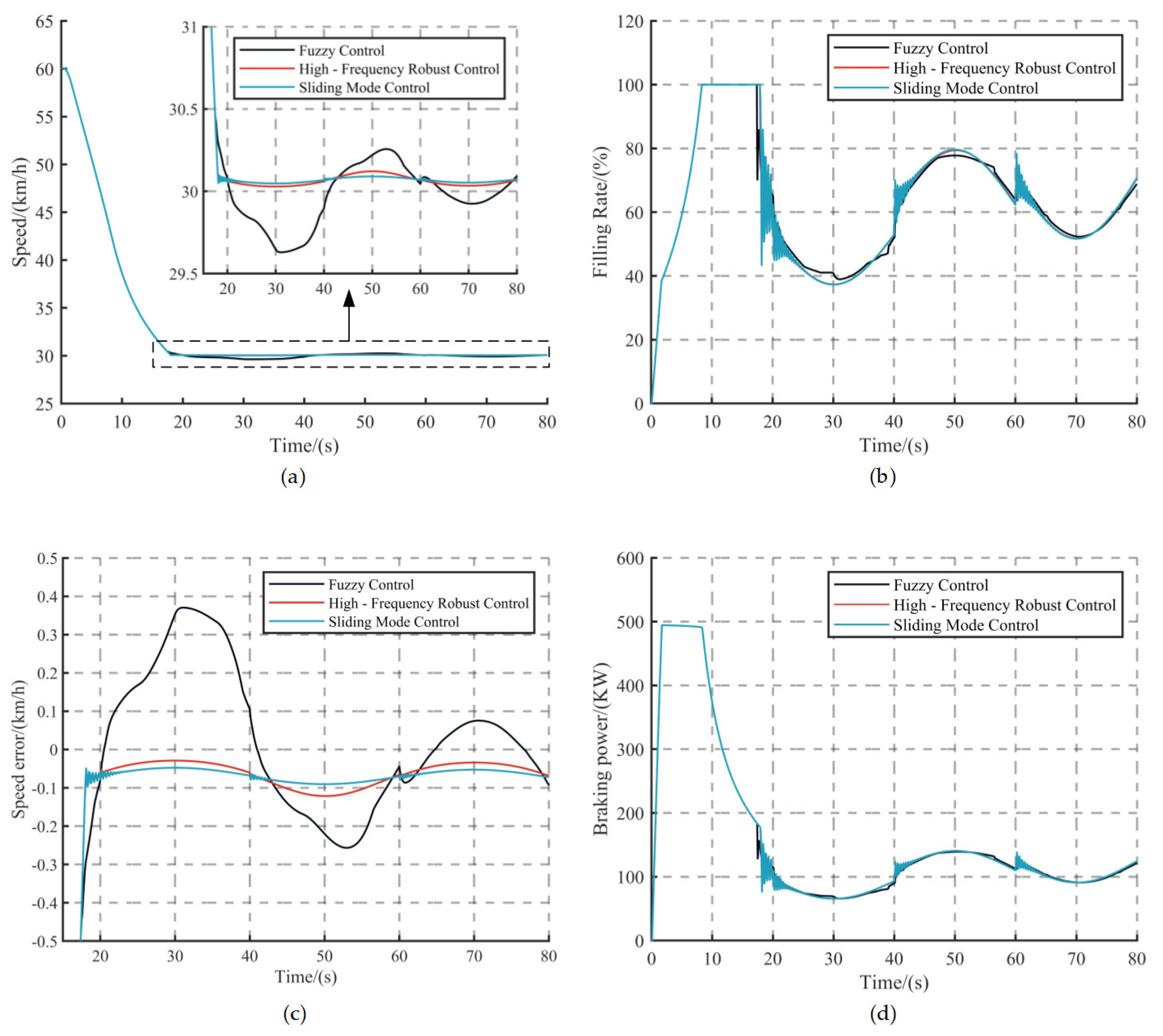
• When the heavy-duty vehicle with constant mass is driving on a ramp with a fixed gradient of 6%, the fuzzy controller demonstrates high speed control accuracy with a maximum speed error of 0.0842 km/h. However, when the system is subject to parameter uncertainty, especially when the vehicle mass and the road gradient vary at the same time, the fuzzy controller has a long response time, and the maximum speed error grows to 0.37 km/h, with speed control accuracy that is low. At the same time, the retarder filling rate of the control output also swings to varying degrees. This is owing to the fact that the fuzzy controller relies on empirical and heuristic principles, has weak adaptability to non-matching disturbances, and has a considerable difference in anti-interference characteristics compared with the other two controllers under dynamic settings.
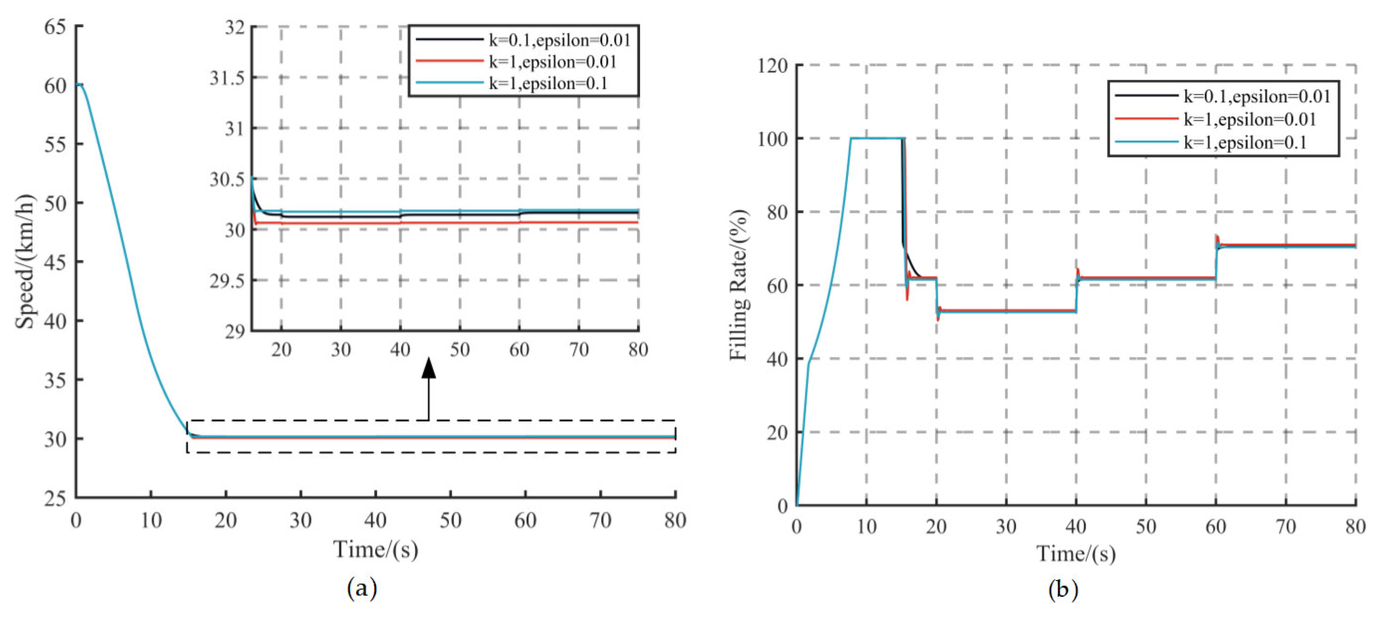
• The sliding mode controller with saturation function shows good speed tracking performance under three simulation conditions, but its control output retarder filling rate signal produces obvious vibration when the vehicle speed reaches near the target speed or the system parameter changes, which is not conducive to the regulation of the hydraulic retarder filling rate in reality. Through simulation analysis, we find that although the saturation function can suppress part of the vibration in traditional sliding mode control, the selection of the boundary layer thickness is more dependent on the system model, and if the value of the boundary layer thickness is too large, it reduces the robustness of the sliding mode control with the saturation function, and if the value of the boundary layer thickness is too small, it increases to increase the degree of vibration in the control output.
• The high-frequency controller has good robustness in the presence of dynamic disturbances in the system. When the vehicle mass and road gradient change, the high-frequency controller speed fluctuation is small; the root mean square error of speed is 0.0683 km/h, compared with the fuzzy controller’s root mean square error of speed of as high as 0.184 km/h. The high-frequency controller under dynamic conditions of interference resistance has better performance. In terms of control output, the high-frequency controller, compared with the sliding mode controller with saturation function, has less fluctuation of the output filling rate when the system parameters are changing and is able to suppress chattering while maintaining strong robustness against perturbation and parameter uncertainty.

Overall, the high-frequency controller is able to achieve fast reaction to changes in system parameters and has strong anti-interference performance under dynamic settings and is suitable for solving the constant-speed braking problem of heavy vehicles travelling downhill for long periods of time. In future work, the joint braking of the service brake, hydraulic retarder, and ABS (Anti-lock Braking System) under various braking conditions will be studied to further improve the control strategy of the vehicle braking system so as to improve the braking safety of the vehicle, and more control methods and experiments of constant-speed braking of the retarder will be considered.

References

1. Tian, J.; Li, D.; Ye, L. Study on braking characteristics of a novel eddy current-hydraulic hybrid retarder for heavy-duty vehicles. IEEE Trans. Energy Convers. 2020, 35, 1658–1666. [Google Scholar] [CrossRef]
2. Wang, Z.; Wei, W.; Chen, X.; Langari, R.; Yan, Q. Comprehensive Evaluation of Hydrodynamic Retarders with Fuzzy Analytic Hierarchy Process and Improved Radar Chart. Machines 2023, 11, 849. [Google Scholar] [CrossRef]
3. Xu, M.; Li, H.Y. Research on constant torque control system design for hydraulic retarder of heavy vehicle. Adv. Mater. Res. 2012, 538, 2493–2499. [Google Scholar] [CrossRef]
4. Gao, Z.; Li, D.; Tian, J.; Ning, K.; Ye, L. Design and performance analysis of a novel radially distributed electrom-agnetic-hydraulic retarder for heavy vehicles. IEEE Trans. Energy Convers. 2021, 37, 892–900. [Google Scholar] [CrossRef]
5. Ding, Z.; Zhou, L.; Xu, J.; Tong, J. Vehicle Retarders: A Review. IEEE Access 2023, 11, 102757–102767. [Google Scholar] [CrossRef]
6. Tan, K.K.; Putra, A.S. Servo Hydraulic and Pneumatic Drive. In Drives and Control for Industrial Automation; Springer: London, UK, 2011; pp. 9–44. [Google Scholar]
7. Zhang, K.; Shang, H.; Xu, J.; Niu, J.; Yue, Y. Testing and performance analysis of an integrated electromagnetic and hydraulic retarder for heavy-duty vehicles. Eng. Appl. Artif. Intell. 2023, 126, 106906. [Google Scholar] [CrossRef]
8. Xue, M.; Fu, Y.; Geng, X.; Sun, S.; Lei, Y. Integration analysis model of oil-charging system about parallel hydraulic retarder and its response characteristic. Eng. Sci. Technol. Int. J. 2024, 53, 101685. [Google Scholar] [CrossRef]
9. Wu, C.; Guo, X.; Yang, B.; Pei, X.; Guo, S. Hydraulic retarder torque control for heavy duty vehicle longitudinal control. Int. J. Heavy Veh. Syst. 2019, 26, 854–871. [Google Scholar] [CrossRef]
10. Mu, H.; Fu, J.; Wu, Z.; Zhu, Y.; Wei, W.; Yan, Q. Optimization on parallel control of PID and fuzzy in constant-speed braking process with a hydrodynamic retarder. In Proceedings of the 2019 IEEE 8th International Conference on Fluid Power and mechatronics (FPM), Wuhan, China, 10–13 April 2019; pp. 1175–1188. [Google Scholar]
11. Huang, J.; Li, C.; Ling, Z.; Chen, Y.; Ma, X. Study on Pivotal Factors to Breaking Torque of Hydrodynamic Retarder. In ICLEM 2010: Logistics for Sustained Economic Development: Infrastructure, Information, Integration; Asce: Reston, VA, USA, 2010; pp. 1353–1360. [Google Scholar]
12. Yan, J.; Guo, X.; Tan, G.; Yang, T.; Zhou, D. Co-Simulation Based Hydraulic Retarder Braking Control System; 0148-7191 SAE Technical Paper; SAE: Warrendale, PA, USA, 2009. [Google Scholar]
13. Zhang, Y. Experimental analysis of heavy vehicle hydraulic retarder during downhill driving. Int. J. Veh. Struct. Syst. 2019, 11, 393–399. [Google Scholar] [CrossRef]
14. Mu, H.; Yan, Q.; Wei, W. Study on influence of inlet and outlet flow rates on oil pressures and braking torque in a hydrodynamic retarder. Int. J. Numer. Methods Heat Fluid Flow 2017, 27, 2544–2564. [Google Scholar] [CrossRef]
15. Mu, H.; Wei, W.; Kong, L.; Zhao, Y.; Yan, Q. Braking characteristics integrating open working chamber model and hydraulic control system model in a hydrodynamic retarder. Proc. Inst. Mech. Eng. Part C J. Mech. Eng. Sci. 2019, 233, 1952–1971. [Google Scholar] [CrossRef]
16. Wei, W.; Tao, T.L.; Chen, X.Q.; Xie, W.H.; Wang, Z.; Yan, Q.D. Research on Braking Performance Prediction and Torque Control of Hydrodynamic Retarder Considering Temperature. In Proceedings of the 2023 9th International Conference on Fluid Power and Mechatronics (FPM), Lanzhou, China, 18–21 August 2023; pp. 1–11. [Google Scholar]
17. Zheng, H.; Lei, Y.; Song, P. Designing the main controller of auxiliary braking systems for heavy-duty vehicles in nonemergency braking conditions. Proc. Inst. Mech. Eng. Part C J. Mech. Eng. Sci. 2018, 232, 1605–1615. [Google Scholar] [CrossRef]
18. Li, L.; Ma, W.X.; Cai, W.; Chu, Y.X.; Song, J.J.; Zhang, Y. Control system analysis of hydrodynamic retarder of heavy truck. Adv. Mater. Res. 2013, 619, 406–409. [Google Scholar] [CrossRef]
19. Liu, Z.; Zheng, H.; Xu, W.; Yu, Z. A Downhill Brake Strategy Focusing on Temperature and Wear Loss Control of Brake Systems; 0148-7191 SAE Technical Paper; SAE: Warrendale, PA, USA, 2013. [Google Scholar]
20. Lei, Y.; Song, P.; Zheng, H.; Fu, Y.; Li, X.; Song, B. Application of fuzzy logic in constant speed control of hydraulic retarder. Adv. Mech. Eng. 2017, 9, 1687814017690956. [Google Scholar] [CrossRef]
21. Li, J.; Cai, Z.; Jia, Z. Simulation of constant speed control on coach hydraulic retarder on special weather condition. Syst. Simul. 2014, 26, 2765–2769. [Google Scholar] [CrossRef]
22. Chen, X.; Ao, K.; Liu, X.; Zhang, Q. Simulation research on vehicle with hydraulic retarder constant speed control strategy. Mach. Tool Hydraul. 2019, 47, 160–165. [Google Scholar] [CrossRef]
23. Cheng, N.B.; Guan, L.W.; Wang, L.P.; Han, J. Chattering reduction of sliding mode control by adopting nonlinear saturation function. Adv. Mater. Res. 2011, 143, 53–61. [Google Scholar] [CrossRef]
24. Laghrouche, S.; Plestan, F.; Glumineau, A. Higher order sliding mode control based on integral sliding mode. Automatica 2007, 43, 531–537. [Google Scholar] [CrossRef]
25. Chen, W.H.; Yang, J.; Guo, L.; Li, S. Disturbance-observer-based control and related methods—An overview. IEEE Trans-Actions Ind. Electron. 2015, 63, 1083–1095. [Google Scholar] [CrossRef]
26. Zheng, H.; Lei, Y.; Song, P. Design of a filling ratio observer for a hydraulic retarder: An analysis of vehicle thermal management and dynamic braking system. Adv. Mech. Eng. 2016, 8, 1687814016674098. [Google Scholar] [CrossRef]
27. Yan, Q.D.; Zou, B.; Wei, W. Research on braking performance calculation model of two-phase flow in hydraulic retarder cascade. Beijing Ligong Daxue Xuebao Trans. Beijing Inst. Technol. 2011, 31, 1396–1400. [Google Scholar]
28. Utkin, V.I. Sliding Modes in Control and Optimization; Springer Science & Business Media: Berlin/Heidelberg, Germany, 2013. [Google Scholar]
Figure 1. Structure of the retarder control system.
Applsci 15 07058 g001
Figure 2. Mounting positions of hydraulic retarder.
Applsci 15 07058 g002
Figure 3. Vehicle slowing downhill control process.
Applsci 15 07058 g003
Figure 4. Force analysis of downhill-traveling vehicle.
Applsci 15 07058 g004
Figure 5. Overall simulation architecture.
Applsci 15 07058 g005
Figure 6. Feedback control system with the controller.
Applsci 15 07058 g006
Figure 7. Schematic diagram of control structure.
Applsci 15 07058 g007
Figure 8. Vehicle mass conditions in the simulation: (a) Fixed vehicle mass, (b) Varying vehicle mass.
Applsci 15 07058 g008
Figure 9. Road slope conditions in the simulation: (a) Fixed slope, (b) Sinusoidal change slope.
Applsci 15 07058 g009
Figure 10. Simulation results of controller with different control parameters: (a) Vehicle speed, (b) Hydraulic retarder filling rate.
Applsci 15 07058 g010
Figure 11. Simulation results under C1 conditions: (a) Vehicle speed, (b) Hydraulic retarder filling rate, (c) Vehicle speed error and (d) Braking power of hydraulic retarder.
Applsci 15 07058 g011
Figure 12. Simulation results under C2 conditions: (a) Vehicle speed, (b) Hydraulic retarder filling rate, (c) Vehicle speed error and (d) Braking power of hydraulic retarder.
Applsci 15 07058 g012
Figure 13. Simulation results under C3 conditions: (a) Vehicle speed, (b) Hydraulic retarder filling rate, (c) Vehicle speed error and (d) Braking power of hydraulic retarder.
Applsci 15 07058 g013