A Joint Decoherence-Based AOA and TDOA Positioning Approach for Interference Monitoring in Global Navigation Satellite System

Abstract

Global navigation satellite system (GNSS) has been widely used in many fields due to their low cost and high positioning accuracy. Because of the open frequency of navigation signals, the low power of navigation signals, and the growing reliance of many modern wireless systems on satellite-based navigation, GNSS performance may be easily affected by interference signals. Monitoring and troubleshooting of interference sources are important means to guarantee the normal use of satellite navigation applications and are an important part of GNSS operation in complex electromagnetic environments; however, traditional angle of arrival (AOA) algorithms cannot efficiently operate with coherent signals, so a decoherence-based orientation scheme is proposed to optimize the AOA algorithm. Furthermore, a joint AOA and time difference of arrival (TDOA) interference localization algorithm is proposed for problems such as the lack of accuracy in a single interference source localization algorithm. Numerical simulation results show that decoherence-based AOA localization can be well applied to various interference signals, and the accuracy of the joint AOA and TDOA interference localization algorithm is higher than that of single-method interference localization. In addition, the physical verification further verifies the usability and reliability of the GNSS interference source positioning algorithm proposed in this paper.

1. Introduction

With the advantages of global coverage, all-weather service, multiple functions, high accuracy, and simple operation, satellite navigation is now widely used in all aspects of social life. In the Global Air Navigation Plan (GANP) released by ICAO in 2016, it is clearly pointed out that GNSS is an important foundation of modern air navigation systems and an important means of enhancing the safety level and service quality of global air navigation. As an important infrastructure, satellite navigation is an important support system for high-tech warfare in the age of information [1]. However, due to the openness of navigation signal frequencies, the low-power characteristics of navigation signals, and the growing dependence of many modern wireless systems on satellite-based navigation, external interference can easily affect the normal operation of satellite navigation systems. As recently noted in the International Air Transport Association (IATA) Safety Report and the European Control Voluntary Air Traffic Management (ATM) Incident Reporting System, the number and sources of GNSS interferences have grown alarmingly over the past few years [2].

Once the satellite navigation receiver locates incorrectly or loses the ability to locate due to interference from satellite navigation signals, it will produce incalculable consequences in military and civil fields. Therefore, the study of satellite navigation interference technology is of great significance [3,4,5,6,7]. However, at present, there are few research studies focusing on satellite navigation jamming technology; the research is mainly based on the evaluation of anti-jamming algorithms and the testing of environmental conditions. Therefore, more research is necessary on satellite navigation interference technology. Satellite navigation jamming mainly includes unintentional jamming and intentional jamming. However, since the operating frequency band of unintentional interference is usually inconsistent with the carrier frequency band of satellite navigation signals, it has little impact on satellite navigation signals. Intentional interference is more harmful to satellite navigation signals and mainly includes suppression interference and deception interference. Suppression interference and deception interference can be classified in many ways according to their different characteristics. Summarizing satellite navigation jamming technology from different classification perspectives helps us to improve the shortcomings of existing satellite navigation jamming technology.

Existing research on satellite navigation interference sources positioning mainly focuses on suppressing interference, and its positioning method mostly adopts the classical two-step positioning [8]. The first step is to intercept the interference signal through the receiver, process the original signal, and estimate the parameters related to the location of the interference source, such as time of arrival (TOA), frequency difference of arrival (FDOA), TDOA, AOA, etc.al (FDOA), angle of arrival (AOA), etc. [9,10]. The second step is to establish the equation between the relevant parameters and the position of the interference source, and then to solve the equation to obtain the position information of the interference source [11]. In addition, there are also methods to locate the interference source using parameters such as the dry signal ratio of the receiver [12]. Reference [13] introduces a modified pole representation that utilizes the angle of arrival to uniformly localize the source without considering whether it is close or far away. A general closed-form formulation of the Cramér–Rao lower bound (CRLB) for hybrid time-of-arrival/angle-of-arrival (TOA/AOA) target localization is presented in Reference [14]. For a given localization scenario, it is theoretically demonstrated that the optimal accuracy of the joint TOA/AOA scheme outperforms any of the TOA and AOA schemes. Reference [15] designs a convex rank unconstrained semi-finite programming (RUSDP) algorithm to obtain a unified solution for TDOA-based near-field and far-field localization by assuming that the signal propagation velocity is unknown.

However, traditional AOA localization has certain shortcomings [16]. Because of multipath transmission and other effects, AOA localization makes it difficult to lateralize coherent signals. In addition, the measurement accuracy of a single-method interference localization algorithm is often insufficient and has a large error. When more base stations are monitored, solving the position equation is more computationally intensive, and the equation is often nonlinear, requiring an optimal solution to be found. However, it is difficult to find accurate results with traditional methods. Therefore, we propose a joint AOA and TDOA interference localization scheme, where the direction measurement uses decoherence to solve the shortcoming of AOA being unable to measure coherent signals, and the least squares method is used to solve the system of position equations. Numerical simulations show that the scheme can achieve accurate interference localization and can be applied to various interference signals. Moreover, the physical verification further verifies the usability and reliability of the proposed scheme.

The main contributions of this paper are as follows:

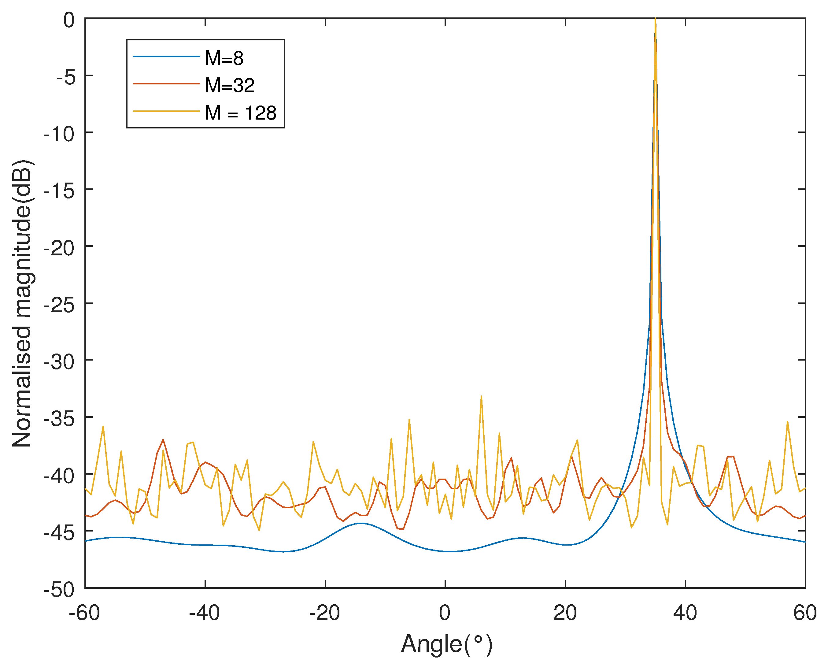
• A decoherence-based AOA-solving algorithm is proposed, which effectively addresses the problem that coherent signals cannot be directionally measured and is applicable to narrowband interference.
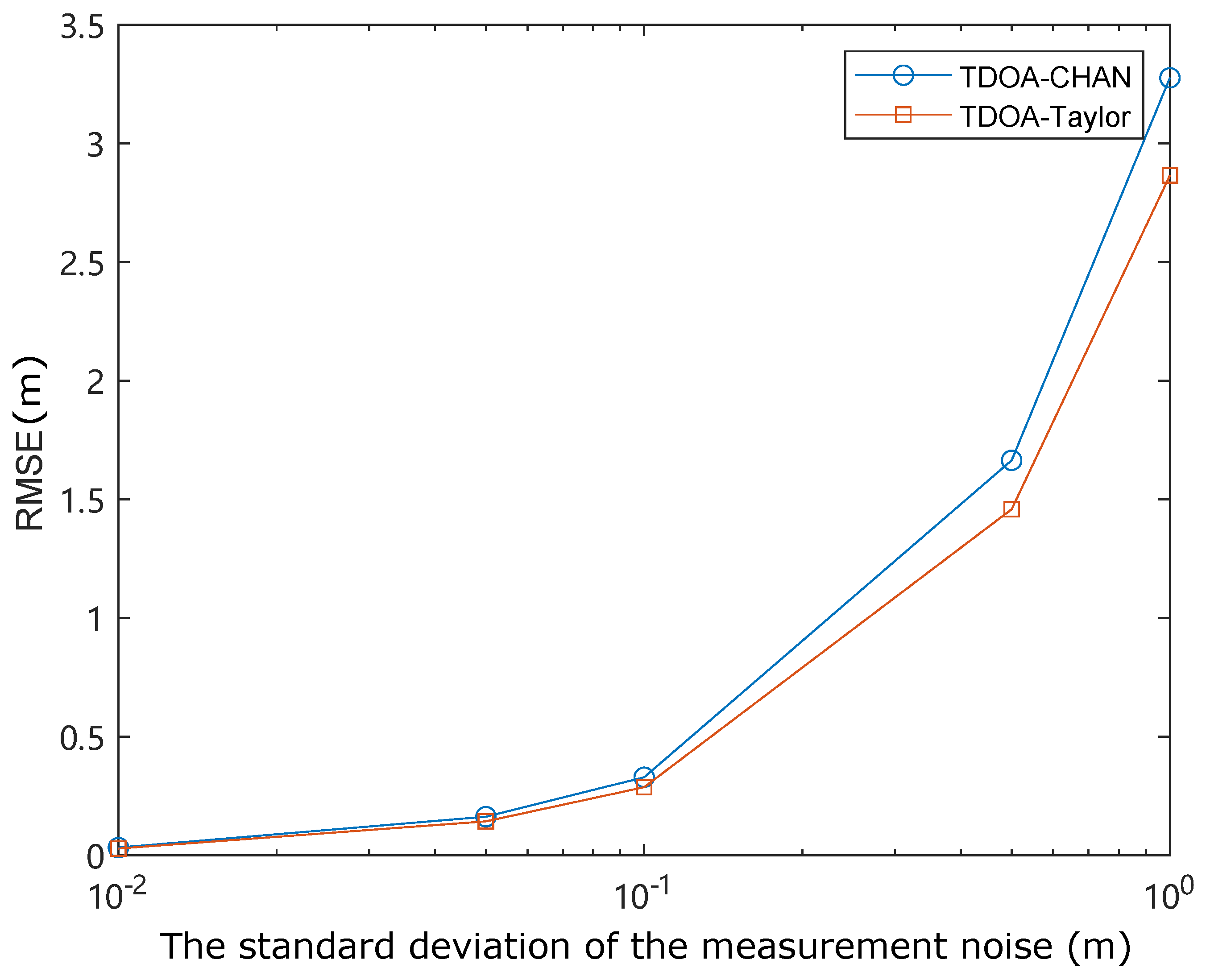
• A TDOA solving algorithm based on the least squares method is proposed, and the simulation results show that this solving method is better than the maximum likelihood estimation algorithm.
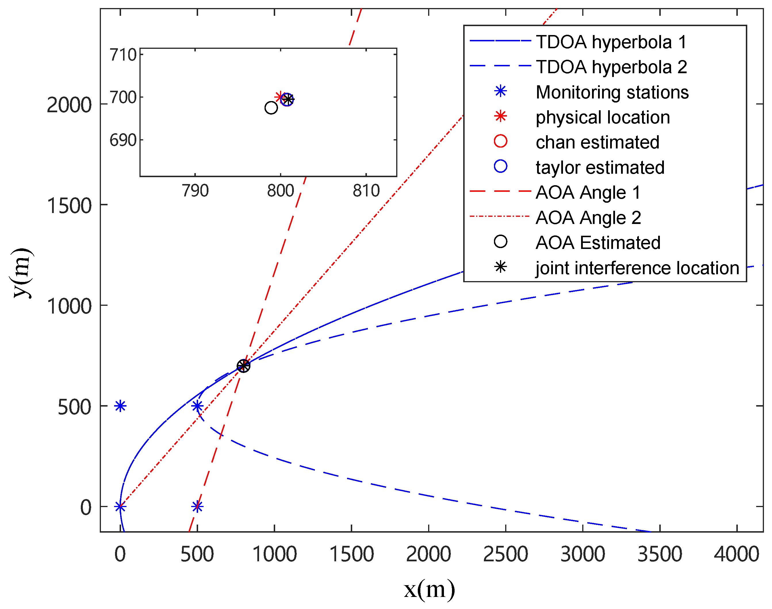
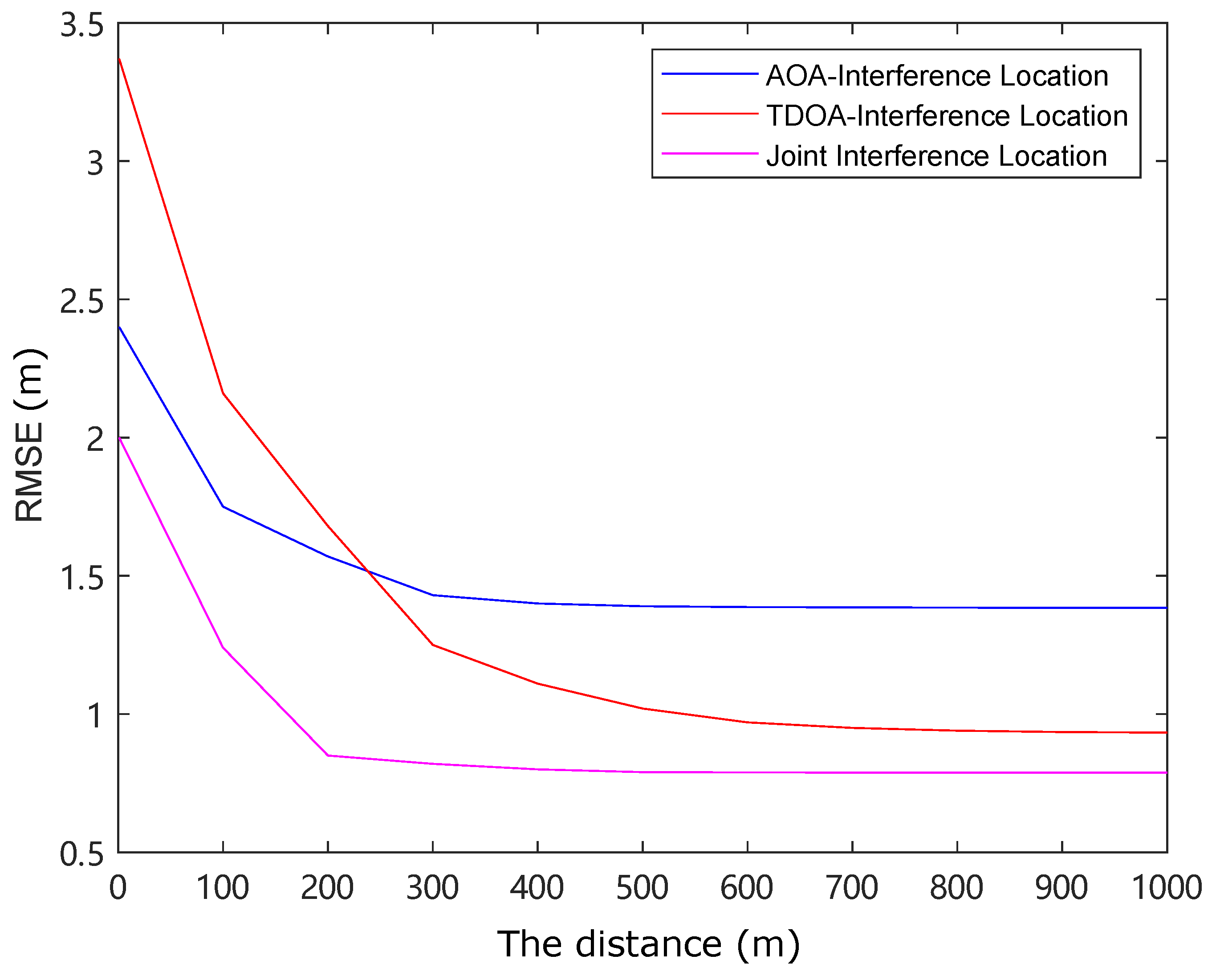
• A joint AOA and TDOA localization algorithm is proposed, and the simulation results show that the joint localization algorithm is better than the single localization algorithm with higher accuracy and better robustness.

This paper is structured as follows. Section 1 presents a literature review of the related field, Section 2 presents the principle of the proposed algorithm, Section 3 analyzes the results of the proposed algorithm, Section 4 analyzes the semi-physical simulation results of the proposed algorithm and Section 5 presents the conclusion.

2. The Joint Positioning Approach

2.1. Decoherence-Based AOA Positioning Scheme

The MUSIC (multi-signal classification) algorithm is a subspace-based high-resolution method for AOA estimation. MUSIC exploits the properties of the covariance matrix of the received signal vector to estimate the AOA of input signals impinging on a receiver array. The MUSIC algorithm is unable to directionally measure coherent signals, due to the effects of multipath transmission, etc., multiple correlated narrowband interferences are simultaneously incident on the array antenna from different directions, at which time the covariance matrix $R_{xx}$ of the data received by the array antenna will suffer from rank loss and the boundaries between the noise subspace and the signal subspace will become fuzzy, with the existence of array steering vector $a^H\left(\varphi \right)\ne O^T$, where $\varphi ={\varphi }_1,{\varphi }_2,\dots ,{\varphi }_p$ represent the AOAs of p far-field interference signals and, therefore, the MUSIC algorithm is not able to directly measure the coherent narrowband interference [17].

Assuming that the array antenna receives p far-field signals at the same time as an M-element direction-finding array antenna in the far-field. The autocorrelation matrix $R_{xx}$ of the array antenna’s output data under ideal conditions is as follows:

$$\begin{array}{cc}\hfill & R_{xx}=E\left\{x\left[k\right]x^H\left[k\right]\right\}\hfill \\ \hfill & =\mathrm{AE}\left\{\mathrm{s}\left[\mathrm{k}\right]{\mathrm{s}}^{\mathrm{H}}\left[\mathrm{k}\right]\right\}{\mathrm{A}}^{\mathrm{H}}+{\sigma }^2\mathrm{I}\hfill \\ \hfill & ={\mathrm{APA}}^{\mathrm{H}}+{\sigma }^2\mathrm{I}\hfill \end{array}$$

(1)

where $A=\left[a\left({\varphi }_1\right),a\left({\varphi }_2\right),\dots ,a\left({\varphi }_p\right)\right]$ is the array flow matrix of the array antenna, ${\sigma }^2$ is the Korst noise power, and I is the unit matrix. In particular, $x\left[k\right]$ is the array antenna’s output data vector for the k-th interference signal, s[k] is the k-th interference signal vector, and P represents the covariance matrix of $s\left[k\right]$.

However, when two of the signals are correlated, the rank of the signal subspace will be reduced to P−1. In order to solve the rank loss, we introduce a nonlinearly correlated array vector into it, and for a uniform linear array, the “inverse array vector” can be chosen as the vector to be introduced.

Therefore, for an M-element uniform linear antenna array, the inverse covariance matrix $R_B$ of $R_{xx}$ is as follows:

$$\begin{array}{cc}& R_B=J{R}_{xx}^{\ast }J\hfill \\ & =A{\mathrm{\Phi }}^{-(M-I)}P{\mathrm{\Phi }}^{-(M-I)}{A}^H+{\sigma }^{2}I\hfill \end{array}$$

(2)

where $\mathrm{\Phi }$ is the diagonal matrix whose diagonal elements are $e^{jm\varphi }(m=1,2,\dots ,M)$, and J is the substitution matrix of M × M.

Averaging over $R_{xx}$ and $R_B$, the positive and negative array covariance matrices $R_{FB}$ can be obtained as follows:

$$\begin{array}{cc}\hfill & R_{FB}={\displaystyle \frac{1}{2}}(R_{xx}+R_B)\hfill \\ \hfill & ={\displaystyle \frac{1}{2}}(R_{xx}+J{R}_{xx}^{\ast }J)\hfill \\ \hfill & =A\tilde{P}{A}^H+{\sigma }^{2}I\hfill \end{array}$$

(3)

Perform a feature decomposition of $R_{FB}$ as follows:

$$R_{FB}=U\times \sum \times U^H$$

(4)

where $\mathrm{\Sigma }$ is the diagonal matrix consisting of M eigenvalues of $R_{FB}$ and U is the feature matrix of $R_{FB}$.

A is a column-full rank matrix, so that $\mathrm{rank}\left(\mathrm{A}\tilde{\mathrm{P}}\mathrm{A}\right)=\mathrm{rank}\left(\tilde{\mathrm{P}}\right)=\tilde{\mathrm{P}}$, if $\tilde{P}<\mathrm{M}$, we have the following:

$$\begin{array}{cc}& \mathrm{U}\times \mathrm{A}\tilde{\mathrm{P}}{\mathrm{A}}^{\mathrm{H}}\times {\mathrm{U}}^{\mathrm{H}}=\sum \hfill \\ & =\mathrm{diag}\{{\mathrm{a}}_1^2,\dots ,{\mathrm{a}}_{\tilde{\mathbf{P}}}^2,0,\dots ,0\}\hfill \end{array}$$

(5)

where $a_1^2$ to $a_{\tilde{P}}^2$ are the eigenvalues of the autocorrelation matrix $A\tilde{P}A$.

Multiply both sides of $R_{FB}$ simultaneously by U, we can obtain the eigenvalues ${\lambda }_i$ of $R_{FB}$ as [18]:

$${\mathrm{U}}^{\mathrm{H}}{\mathrm{R}}_{\mathrm{FB}}\mathrm{U}=\mathrm{diag}\{a_1^2,\dots ,a_{\tilde{p}}^2,0,\dots ,0\}+{\sigma }^2\mathrm{I}$$

(6)

$${\lambda }_{\mathrm{i}}=\{\begin{array}{cc}{a}_i^2+{\sigma }^2& i=1,2,\dots ,\tilde{\mathbb{P}}\\ {\sigma }^2& i=\tilde{\mathbb{P}}+1,\dots ,\mathbb{M}\end{array}$$

(7)

The first P eigenvalues of $R_{FB}$ contain both the received signal and the noise and have large values; the last M-P eigenvalues of $R_{FB}$ contain only the noise component and have small values. Therefore, the number of signals received by the array antenna can be estimated by observing the eigenvalues of $R_{FB}$.

The eigenvector corresponding to the first P eigenvalues of the $R_{FB}$ is $\mathrm{S}=[s_1,s_2,\dots ,s_p]$, and the space consisting of S is the signal subspace. The eigenvector corresponding to the last M-P eigenvalues of the $R_{FB}$ is $\mathrm{G}=[{\mathrm{g}}_1,{\mathrm{g}}_2,\dots ,{\mathrm{g}}_{\mathrm{M}-\mathrm{P}}]$, and the space consisting of g is the noise subspace $\mathrm{range}\left(\mathrm{G}\right)$. $\mathrm{range}\left(\mathrm{S}\right)$ and $\mathrm{range}\left(\mathrm{G}\right)$ can be represented as follows:

$$\mathrm{range}\left(\mathrm{S}\right)=\mathrm{span}\{{\mathrm{s}}_1,{\mathrm{s}}_2,\dots ,{\mathrm{s}}_{\mathrm{P}}\}$$

(8)

$$\mathrm{range}\left(\mathrm{G}\right)=\mathrm{span}\{{\mathrm{g}}_1,{\mathrm{g}}_2,\dots ,{\mathrm{g}}_{\mathrm{P}}\}$$

(9)

$P_s=S{S}^H$ is called the projection matrix on the signal subspace, and ${\mathrm{GG}}^{\mathrm{H}}=\mathrm{I}-{\mathrm{P}}_{\mathrm{s}}$ is called the orthogonal projection matrix on the signal subspace.

Multiply G to the right of $R_{FB}$, we can obtain the following:

$$\begin{array}{cc}& {\mathrm{R}}_{\mathrm{FB}}\mathrm{G}={\mathrm{APA}}^{\mathrm{H}}+{œ}^2\mathrm{G}\hfill \\ \hfill =& \left[\mathrm{S}\mathrm{G}\right]\Sigma \left[\begin{array}{c}{\mathrm{S}}^{\mathrm{H}}\\ {\mathrm{G}}^{\mathrm{H}}\end{array}\right]\mathrm{G}=\left[\mathrm{S}\mathrm{G}\right]\Sigma \left[\begin{array}{c}\mathrm{O}\\ \mathrm{I}\end{array}\right]={\sigma }^2\mathrm{G}\hfill \end{array}$$

(10)

Therefore, the following can be inferred:

$${\mathrm{GAPA}}^{\mathrm{H}}\mathrm{G}=\mathrm{O}$$

(11)

And the sufficient condition for Equation (11) to hold is as follows:

$${\mathrm{A}}^{\mathrm{H}}\mathrm{G}=\mathrm{O}$$

(12)

Based on Equations (11) and (12), we have the following:

$${\mathrm{a}}^{\mathrm{H}}\left(\varphi \right)\mathrm{G}={\mathrm{O}}^{\mathrm{T}}\varphi ={\varphi }_1,{\varphi }_2,\dots ,{\varphi }_p$$

(13)

Therefore, the spatial spectrum $P_{Music}$ of the received signal is as follows:

$$\begin{array}{cc}\hfill {\mathrm{P}}_{\mathrm{Music}}\left(\varphi \right)& ={\displaystyle \frac{1}{{\mathrm{a}}^{\mathrm{H}}\left(\varphi \right){\mathrm{GG}}^{\mathrm{H}}\mathrm{a}\left(\varphi \right)}}\hfill \\ & ={\displaystyle \frac{1}{{\mathrm{a}}^{\mathrm{H}}\left(\varphi \right)(\mathrm{I}-{\mathrm{SS}}^{\mathrm{H}})\mathrm{a}\left(\varphi \right)}}\hfill \end{array}$$

(14)

When $\varphi ={\varphi }_1,{\varphi }_2,\dots ,{\varphi }_p$, the value of $P_{Music}$ is large; otherwise, the value of $P_{Music}$ is small. Find the P guiding vectors that make the $P_{Music}$ obtain an extreme value, where the angle corresponding to $\mathit{a}\left({\varphi }_1\right),\mathit{a}\left({\varphi }_2\right),\dots ,\mathit{a}\left({\varphi }_P\right)$ is the angle of incidence of the interfering signal.

Finally, the AOA value for a single monitoring base station is as follows:

$$\mathrm{A}=arcsin{\displaystyle \frac{\mathsf{\Delta }{\varphi }_{12}}{d}}{\displaystyle \frac{c}{2\pi f_{carr}}}$$

(15)

where $\mathsf{\Delta }{\varphi }_{12}$ is the phase difference between two antennas, c is the speed of light, and $f_{carr}$ is the carrier frequency.

Taking two monitoring base stations as an example, the coordinates of the base stations are $(x_1,y_1)$ and $(x_2,y_2)$. According to the sine theorem, the location of the interference source can be obtained as follows:

$$\mathrm{X}={\displaystyle \frac{{\mathrm{LsinA}}_2}{\sin ({\mathrm{A}}_2-{\mathrm{A}}_1)}}{\mathrm{cosA}}_1+{\mathrm{x}}_1\mathrm{Y}={\displaystyle \frac{{\mathrm{LsinA}}_2}{\sin ({\mathrm{A}}_2-{\mathrm{A}}_1)}}{\mathrm{sinA}}_1+{\mathrm{y}}_1$$

(16)

where L is the distance between two monitoring base stations. When there are more than two monitoring base stations, the coordinate equations may be non-linear, and the least squares method can be used to solve the coordinate optimal solution, which will be introduced later.

2.2. Joint TDOA Positioning Program

The location of the interference source can also be estimated by the difference $r_1-r_2=\mathsf{\Delta }{\tau }_{12}c$ in the signal propagation time measured at the spatially displaced receiver.

A common method is to calculate the cross-correlation function between the signals received at each receiver to determine the time difference between them. The inter-correlation function can be expressed as follows:

$${\mathrm{R}}_{x_1{x}_2}\left(\tau \right)=\mathrm{E}[x_1(\mathrm{t}+\tau )·x_2^{\ast }\left(\mathrm{t}\right)]$$

(17)

where E[ ] is the expected value operator and ${\left(\right)}^{\ast }$ is the complex conjugate. However, due to the limited observation time, $R_{x_1{x}_2}\left(\tau \right)$ can only be estimated. The estimation of traversing discrete samples without normalization can be expressed as follows:

$${\widehat{\mathrm{R}}}_{x_1{x}_2}\left(\tau \right)=\sum _{k=0}^{N-\tau -1}{x}_1(k+\tau )·x_2^{\ast }\left(k\right)$$

(18)

where N denotes the total number of digital samples in the original observation interval T; hence, $\mathrm{N}=\mathrm{T}·f_s$, where $f_s$ is the sampling frequency. The value $\tau$ that maximizes the cross-correlation function is the TDOA estimate:

$${\widehat{\tau }}_d=argmax\left[{\widehat{R}}_{x_1{x}_2}\left(\tau \right)\right]$$

(19)

Using discrete-time cross-correlation, the time delay estimate ${\widehat{\tau }}_d$ will be an integer value because the delay is computed at an integer delay determined by the sampling rate of the received signal. If the sampling rate is $f_s$, the inter-correlation time resolution is $1/f_s$, but depending on the sampling rate, the inter-correlation peaks may not fall on the actual discrete samples and, therefore, the discretization of the inter-correlation function must be interpolated to determine the time delay more accurately. Thus, the time delay can be expressed in terms of two components:

$${\tau }_{\mathfrak{d}}=p+\delta$$

(20)

where p is the integer delay associated with the sampling rate, and $\left|\delta \right|\le 0.5T_s$ is the fractional part of the delay.

Parabolic interpolation is a simple interpolation method widely used to improve the accuracy of fitting the optimal peak of the cross-correlation function. The fractional part $\widehat{\delta }$ of the delay estimate can be found by fitting a parabola to three samples of ${\widehat{R}}_{x_1{x}_2}$ around the position of the integer cross-correlation peak, which can be expressed as follows:

$$\widehat{\delta }={\displaystyle \frac{{\widehat{\mathcal{R}}}_{x_1{x}_2}(p+1)-{\widehat{\mathcal{R}}}_{x_1{x}_2}(p-1)}{-{\widehat{\mathcal{R}}}_{x_1{x}_2}(p+1)+2{\widehat{\mathcal{R}}}_{x_1{x}_2}\left(p\right)-{\widehat{\mathcal{R}}}_{x_1{x}_2}(p-1)}}$$

(21)

where p is the integer cross-correlation peak position, ${\widehat{R}}_{x_1{x}_2}\left(p\right)$ is the value of the cross-correlation function peak, and ${\widehat{R}}_{x_1{x}_2}(p-1)$ and ${\widehat{R}}_{x_1{x}_2}(p+1)$ are the values of the cross-correlation function to the left and right of the cross-correlation peak, respectively.

Each TDOA estimation result produces a set of possible position equations. Each TDOA estimation result can be expressed as a set of two-dimensional hyperbolic equations with the coordinates of the interference source located at a point on the hyperbola, and the position equation can be expressed as [19]:

$$\mathsf{\Delta }{\mathbf{t}}_{i,j}·c=\sqrt{{\left({\mathrm{X}}_{\mathrm{i}}-\mathrm{x}\right)}^2+{\left({\mathrm{Y}}_{\mathrm{i}}-\mathrm{y}\right)}^2}-\sqrt{{\left({\mathrm{X}}_{\mathrm{j}}-\mathrm{x}\right)}^2+{\left({\mathrm{Y}}_{\mathrm{j}}-\mathrm{y}\right)}^2}$$

(22)

where (x, y) denotes the position of the transmitter, $(X_i,Y_i)$, $(X_j,Y_j)$ denotes the position of a pair of receivers, i and j satisfy $\mathrm{i}=1,\dots ,N-1$ and $\mathrm{j}=2,\dots ,N$, where N is the number of receivers, $\mathrm{i}\ne \mathrm{j}$, and c is the speed of light, and is the TDOA measurement between receivers. A monitoring system consists of N receivers, where there are N-1 linearly independent TDOA equations, such as $\mathsf{\Delta }{\mathrm{t}}_{1,2}$ and $\mathsf{\Delta }{\mathrm{t}}_{1,3}$. The intersection of two or more hyperbolas generated from three or more TDOA measurements enables estimation of the two-dimensional position of the transmitter.

According to the TDOA estimation, the interference position can be calculated by solving a set of nonlinear requirements. In matrix–vector form, the system of position estimation equations can be expressed as follows:

$$\widehat{\mathbf{d}}=f\left(\theta \right)+e$$

(23)

where $\widehat{d}$ is the vector of noise measurements, $\mathrm{f}\left(\theta \right)$ is the vector of position equations derived on $\mathit{\theta }=\{\mathbf{x},\mathbf{y}\}$, and e is the measurement noise. TDOA position estimation equations are inherently nonlinear and need to be solved iteratively. One way to solve the position equation is to minimize the least squares cost function, which can be defined as follows:

$$\epsilon =\sqrt{{(\widehat{d}-f\left(\theta \right))}^T{C}^{-1}(\widehat{d}-f\left(\theta \right))}\widehat{\theta }=argmin\left(\epsilon \right)$$

(24)

where $\theta$ is the estimate of the parameter that minimizes the cost function and C is the covariance matrix.

Finally, the final interference source localization is obtained by averaging the decoherence AOA localization results and the TDOA localization results as follows:

$$(X,Y)=({\displaystyle \frac{x_{\mathrm{AOA}}+x_{\mathrm{TDOA}}}{2}},{\displaystyle \frac{y_{\mathrm{AOA}}+y_{\mathrm{TDOA}}}{2}})$$

(25)

The estimation accuracy of TDOA is constrained by the bandwidth B of the interference signal to be positioned and the signal-to-noise ratio (SNR) [20]. And the Cramér–Rao lower bound (CRLB) can be approximately expressed as follows:

$${\sigma }_{\mathrm{TDOA}}^2\ge {\displaystyle \frac{c^2}{8{\pi }^2{B}^2·\mathrm{SNR}}}$$

(26)

Equation (26) shows that the TDOA positioning error becomes more pronounced in narrowband interference scenarios. Therefore, a joint decoherence AOA and TDOA localization algorithm is proposed. And the Cramér–Rao bound (CRB) for AOA estimation is given by the following [21]:

$${\sigma }_{AOA}^2\ge {\displaystyle \frac{3{\lambda }^2}{8{\pi }^2{M}^3{d}^{2}SNR}}$$

(27)

where d is the inter-element spacing and $\lambda$ is the wavelength of the positioning interference signal. Inspired by [22,23], the joint AOA and TDOA localization algorithm estimation accuracy can be approximately expressed as follows:

$${\sigma }_{\mathrm{joint}}^2={\displaystyle \frac{{\sigma }_{\mathrm{AOA}}^2·{\sigma }_{\mathrm{TDOA}}^2}{{\sigma }_{\mathrm{AOA}}^2+{\sigma }_{\mathrm{TDOA}}^2}}$$

(28)

Equation (28) shows that the joint localization algorithm is better than the single localization algorithm with higher accuracy and better robustness. When ${\sigma }_{TDOA}^2\approx {\sigma }_{AOA}^2$, the joint positioning accuracy improves by approximately $\sqrt{2}$ times.

In practical applications, AOA and TDOA measurement errors may exhibit correlation due to shared base station clock synchronization errors or overlapping multipath effect regions, requiring correction of the positioning model through a covariance matrix, which refers to 3GPP TR 38.855. When accounting for error correlation, the joint positioning error should be modified as follows:

$${\sigma }_{\mathrm{joint}}^2={\displaystyle \frac{1}{4}}\left[{\sigma }_{\mathrm{AOA}}^2+{\sigma }_{\mathrm{TDOA}}^2-2\rho {\sigma }_{\mathrm{AOA}}{\sigma }_{\mathrm{TDOA}}\right]$$

(29)

where $\rho$ denotes the error correlation coefficient and is defined as the ratio of the covariance of AOA and TDOA errors to the product of their respective standard deviations:

$$\rho ={\displaystyle \frac{{\sum }_{i=1}^N{\sum }_{j>i}^N\mathsf{\Delta }{\theta }_i·\mathsf{\Delta }{\tau }_j}{\sqrt{{\sum }_{i=1}^N{\left(\mathsf{\Delta }{\theta }_i\right)}^2}·\sqrt{{\sum }_{j>i}^N{\left(\mathsf{\Delta }{\tau }_j\right)}^2}}}$$

(30)

where N is the number of base stations, $\mathsf{\Delta }{\theta }_i$ denotes the AOA error of the i-th base station and $\mathsf{\Delta }{\tau }_j$ denotes the TDOA error of the j-th pair base station.

3. Numerical Simulation

To verify the effectiveness of this method, MATLAB 2021b is used as a simulation platform to carry out the verification. In the study of interference effects in satellite navigation systems, additive white Gaussian noise (AWGN) has emerged as the predominant interference mode due to its canonical statistical characteristics and ubiquitous presence. In the experiment, band-limited white noise was generated through equivalent low-pass filtering operations and utilized as the simulated navigation interference source.

Figure 1 shows the results of the decoherence direction-finding scheme for the lateralization of the interference signal. The amplitude measured by the antenna is concentrated in the direction of the interference source of the satellite navigation signal. M is the number of antenna elements, and it can be seen that the larger M is, the more data is received, and the direction-finding amplitude becomes more stable. However, even M = 8 ensures better direction-finding accuracy. This is because the normalized amplitude of the angular antenna direction finding in other directions is minimal. In contrast, the amplitude in the direction of the interference source is very sharp, thus ensuring the accuracy of the AOA direction finding.

When generating the simulation data, it is assumed that the position of the interference source is fixed, the interference transmitting antenna is an omnidirectional antenna, the transmitting power of the interference source is 120 W, and the distance between the interference source and each receiver is 0.2~0.5 km. The bandwidth B of the interference signal is 32.736 MHz. The simulation data are the data of the interference signals received from different interference monitoring base stations, and the receiver position error and ambient noise error should be added to the simulation data for the sake of making the simulation data closer to the real data, where the receiver position error is modeled as zero-mean ${\sigma }_{pos}^2$-variance Gaussian noise in each Cartesian coordinate and the ambient noise error is modeled as AWGN with noise power $P_{noise}=k_{B}TB$, where $k_B$ is the Boltzmann constant, T is the standard noise temperature, and B is the bandwidth of the interference signal.

Figure 2 shows the joint AOA and TDOA localization results. TDOA localization based on least squares (Taylor estimated) and maximum likelihood estimation (Chan estimated) are also illustrated in Figure 2.

It can be seen that both algorithms for solving the position equation achieve good performance. In addition, it can be seen that the joint positioning algorithm achieves better positioning accuracy than the single interference positioning algorithm. The dashed lines in the figure indicate the AOA localization curves and the TDOA localization curves, with each set of curves indicating possible interference source localization locations. This is because both the AOA localization algorithm and the TDOA localization algorithm require the cooperative localization of multiple base stations to achieve accurate localization of the interference source. The localization result of a single base station is a set of possible locations.

Figure 3 compares the error of solving the system of position equations by least squares and maximum likelihood estimation, and it can be seen that, regardless of the size of the noise error, the least squares method for solving the system of position equations is better than the maximum likelihood estimation algorithm.

Regardless of the standard deviation of the measurement noise, the least squares (LS) method performs better than the maximum likelihood estimation (MLE) method for solving position equations, which stem from two principal advantages: (i) enhanced robustness to potential model misspecifications, particularly in handling non-Gaussian measurement noise, and (ii) superior computational stability, as LS provides closed-form solutions that avoid convergence ambiguities inherent to MLE’s iterative optimization. Moreover, the LS framework circumvents the convergence challenges of MLE in non-convex optimization landscapes, avoiding suboptimal local minima or divergent iterations in MLE.

Figure 4 compares the accuracy of the joint AOA and TDOA positioning scheme and the single-method interference positioning. It can be observed that the accuracy of the joint positioning scheme achieves superior accuracy by leveraging complementary spatial and temporal information and mitigating estimation ambiguity. Single-method interference positioning schemes rely solely on either angular or temporal measurements, which are inherently limited by geometric dilution of precision (GDOP) and sensitivity to noise. In contrast, the joint scheme combines AOA’s directional precision with TDOA’s robustness to synchronization errors, effectively constraining the solution space and mitigating individual measurement uncertainties. This fusion not only improves localization consistency but also enhances resilience to multipath effects and sensor placement biases, leading to superior accuracy.

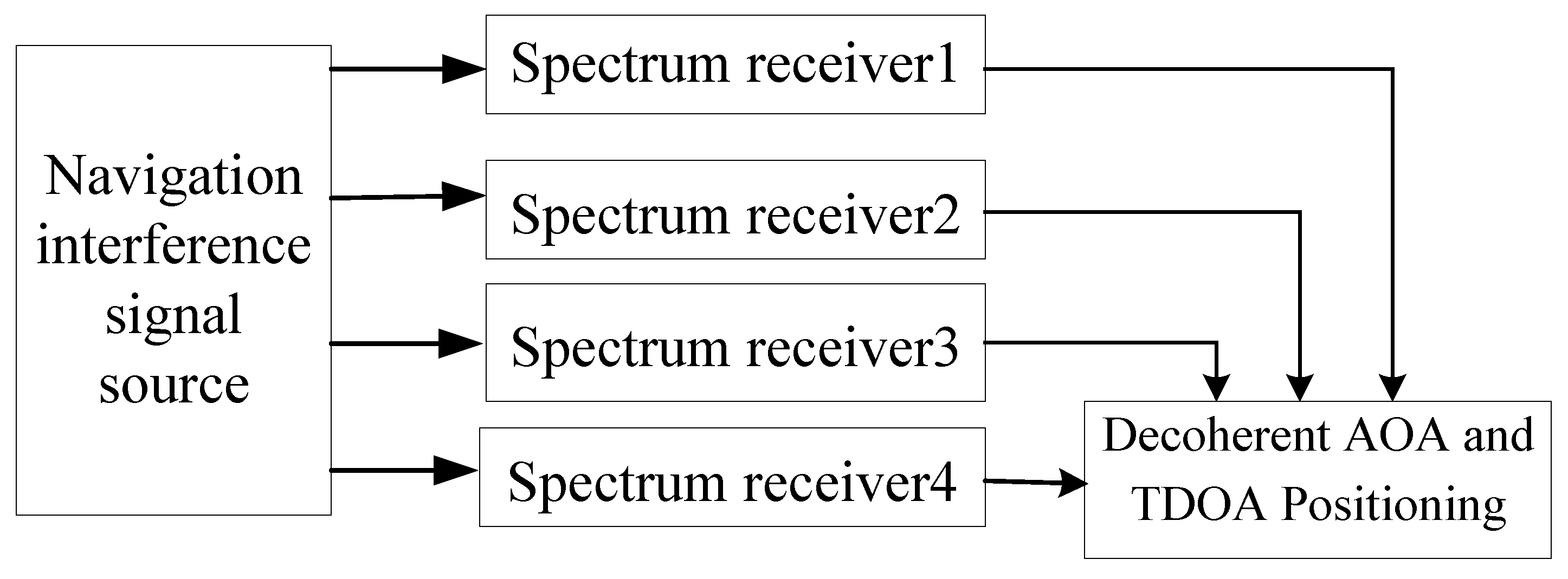
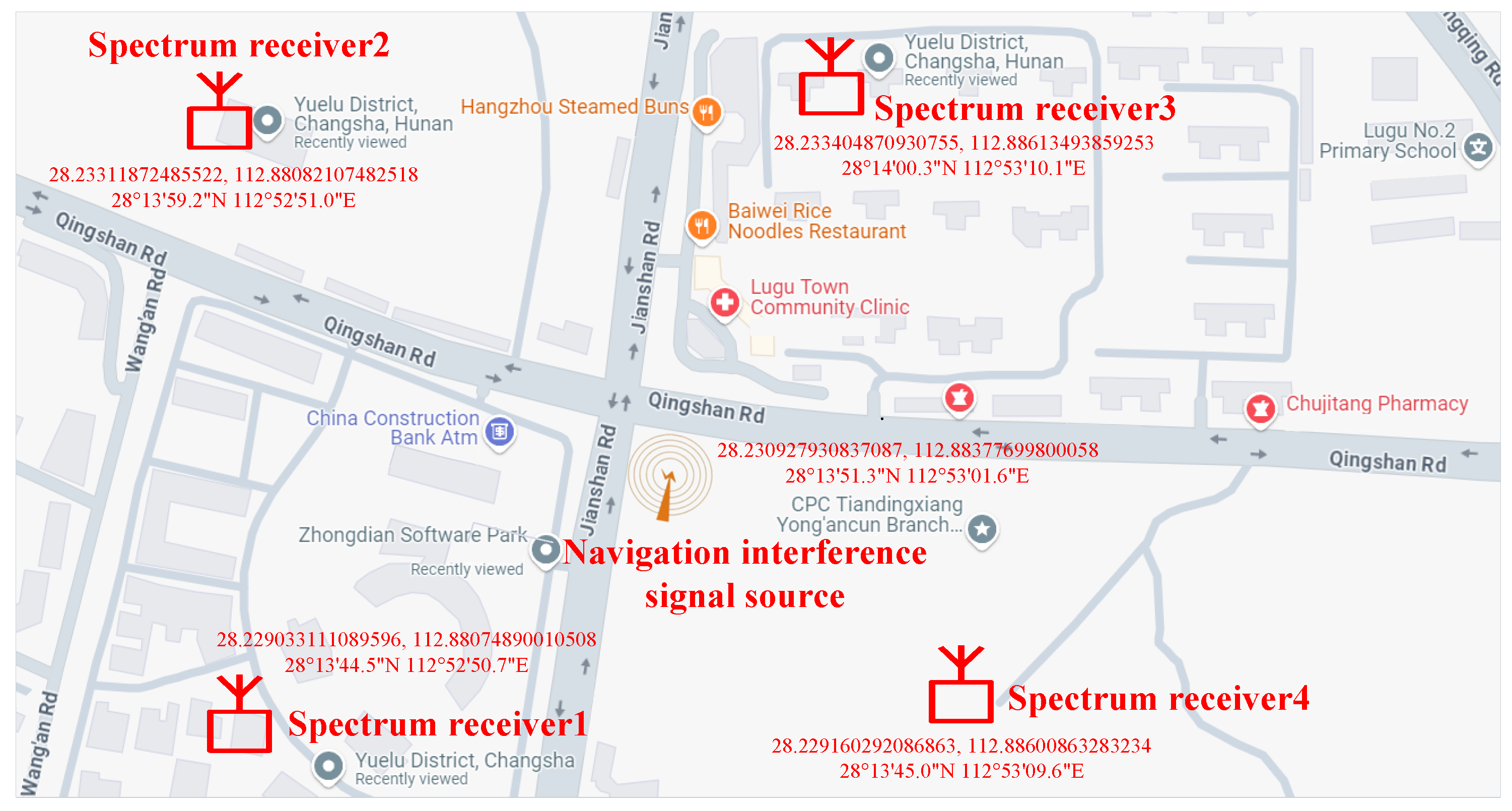
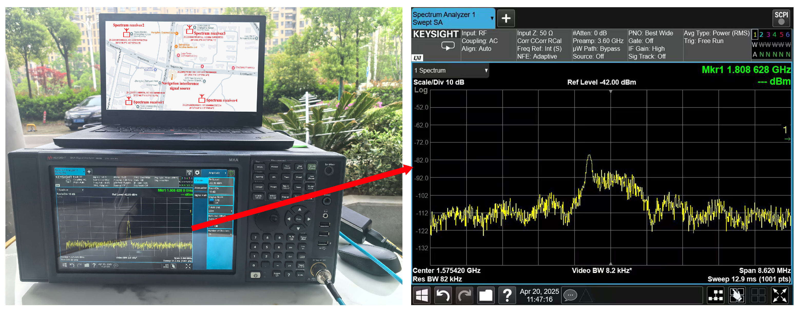
4. Experiment Verification

To further validate the proposed joint decoherence-based AOA and TDOA positioning method, physical verification was performed in a controlled outdoor environment. The experiment employed an interference with a bandwidth of $B=32.736$ MHz and a center frequency of $f_c=1.5479$ GHz. The calibrated transmission power was $P_t=120$ W, which was equivalent to 10 W of equivalent isotropically radiated power (EIRP) after accounting for the attenuator and antenna gain. The low noise amplifier (LNA) saturation power was $-30$ dBm, and the actual received power of $-15$ dBm was measured to be below the saturation level.

The experiment block diagram is shown in Figure 5 and its verification platform is shown in Figure 6, where the interference source was a programmable GNSS jammer, operating at 1.575 GHz (L1/B1C band), with adjustable transmission power (0–150 W) and bandwidth (32.736 MHz). Four spectrum receivers equipped with high-gain omnidirectional antennas and USRP N310 software-defined radios (SDRs) were placed for conducting semi-physical simulation experiments. Moreover, experimental verification parameter settings were configured as follows: the spectrum receiver positions were given in latitude and longitude as (28°13^′59.2^″ N, 112°52^′51.0^″ E), (28°13^′44.5^″ N, 112°52^′50.7^″ E), (28°13^′45.0^″ N, 112°53^′09.6^″ E) and (28°14^′00.3^″ N 112°53^′10.1^″ E), and the interference source position was (28°13^′51.3^″ N, 112°53^′01.6^″ E), with its distances to each base station ranging from 0.2 km to 5 km.

Figure 7 shows the measured angular spectrum for Figure 6, which shows that a navigation interference signal of 1.5479 GHz was detected. The spectrum analyzer was set to an 8.62 MHz span, covering a range from 1.57111 GHz to 1.57973 GHz, with a resolution bandwidth (RBW) of 82 kHz and a video bandwidth (VBW) of 8.2 kHz to reduce noise and improve signal clarity. The symbol * in the right image represents that the VBW displayed on the current screen is set under the manual mode. This setup is tailored for monitoring GNSS interference signals, with a focus on detecting interference or evaluating signal quality in the navigation spectrum. Upon detecting navigation interference signals, the joint decoherence-based AOA and TDOA positioning algorithm was implemented on the USRP N310 SDR platform to realize high-precision calculation of the spatial coordinates of the interference source.

The AOA method yielded interference source position estimates at (28.230917° N, 112.883778° E), with a residual error of 0.39 m from the true location. Using the TDOA method, the estimated interference source position converged to (28.23091° N, 112.88377° E), with a residual error of 0.25 m from the true location. The proposed joint decoherence-based AOA and TDOA positioning method series estimation yielded (28.23092° N, 112.88378° E) with a marginally lower residual error of 0.18 m. It is noted that although only one representative epoch is reported for clarity, multiple repeated trials were conducted under identical conditions. The relative error between the measured positioning coordinates and the simulation-predicted results remained within the 0.6–0.8% range, which further validates the stability and reliability of the proposed approach.

5. Conclusions

In this paper, a joint interference localization scheme based on the decoherence direction-finding method and the least-squares-based TDOA algorithm is proposed. The decoherence algorithm effectively addresses the problem of coherent signals that cannot be oriented and is also well suited to other types of interfering signals. Simulation analysis shows that the scheme can be applied to various interference signals and performs better than a single-method interference localization scheme. The solution error of the least squares method is also smaller than that of the maximum likelihood estimation algorithm.

References

1. Kolomijeca, A.; López-Salcedo, J.A.; Lohan, E.-S.; Seco-Granados, G. GNSS applications: Personal safety concerns. In Proceedings of the 2016 International Conference on Localization and GNSS (ICL-GNSS), Barcelona, Spain, 28–30 June 2016; pp. 1–5. [Google Scholar] [CrossRef]
2. Fokin, G. Interference Suppression Using Location Aware Beamforming in 5G Ultra-Dense Networks. In Proceedings of the 2020 IEEE Microwave Theory and Techniques in Wireless Communications (MTTW), Riga, Latvia, 1–2 October 2020; pp. 13–17. [Google Scholar] [CrossRef]
3. Wendel, J.; Kurzhals, C.; Houdek, M.; Samson, J. An interference monitoring system for GNSS reference stations. In Proceedings of the 2012 15 International Symposium on Antenna Technology and Applied Electromagnetics, Toulouse, France, 25–28 June 2012; pp. 1–5. [Google Scholar] [CrossRef]
4. Gamba, M.T.; Falletti, E. Performance Comparison of FLL Adaptive Notch Filters to Counter GNSS Jamming. In Proceedings of the 2019 International Conference on Localization and GNSS (ICL-GNSS), Nuremberg, Germany, 4–6 June 2019; pp. 1–6. [Google Scholar] [CrossRef]
5. Bethi, P.; Pathipati, S.; P, A. GNSS Intentional Interference Mitigation via Average KF Innovation and Pseudo Track Updation. In Proceedings of the 2020 IEEE 17th India Council International Conference (INDICON), New Delhi, India, 10–13 December 2020; pp. 1–5. [Google Scholar] [CrossRef]
6. Yu, X.; Tu, L.; Yang, Q.; Yu, M.; Xiao, Z.; Zhu, Y. Hybrid Beamforming in mmWave Massive MIMO for IoV with Dual-Functional Radar Communication. IEEE Trans. Veh. Technol. 2023, 72, 9017–9030. [Google Scholar] [CrossRef]
7. Yu, X.; Yang, Q.; Xiao, Z.; Chen, H.; Havyarimana, V.; Han, Z. A Precoding Approach for Dual-Functional Radar-Communication System with One-Bit DACs. IEEE J. Sel. Areas Commun. 2022, 40, 1965–1977. [Google Scholar] [CrossRef]
8. Liu, R.; Yang, Z.; Chen, Q.; Liao, G.; Zhen, W. GNSS Multi-Interference Source Centroid Location Based on Clustering Centroid Convergence. IEEE Access 2021, 9, 108452–108465. [Google Scholar] [CrossRef]
9. Chang, Y.T. Simulation and Implementation of an Inte-grated TDOA/AOA Monitoring System for Preventing Broadcast Interference. J. Appl. Res. Technol. 2014, 12, 1051–1062. [Google Scholar] [CrossRef]
10. An, D.J.; Moon, C.-M.; Lee, J.-H. Derivation of an explicit expression of an approximate location estimate in AOA-based localization. In Proceedings of the 2017 7th IEEE International Symposium on Microwave, Antenna, Propagation, and EMC Technologies (MAPE), Xi’an, China, 24–27 October 2017; pp. 552–555. [Google Scholar] [CrossRef]
11. Ding, R.; Qian, Z.-h.; Wang, X. UWB Positioning System Based on Joint TOA and DOA Estimation. J. Electron. Inf. Technol. 2010, 32, 313–317. (In Chinese) [Google Scholar] [CrossRef]
12. Shao, S.; Liang, Q.; Deng, K.; Tang, Y. Optimal location of the base station based on measured interference power. In Proceedings of the 2015 IEEE International Wireless Symposium (IWS 2015), Shenzhen, China, 30 March–1 April 2015; pp. 1–3. [Google Scholar] [CrossRef]
13. Wang, Y.; Ho, K.C. Unified Near-Field and Far-Field Localization for AOA and Hybrid AOA-TDOA Positionings. IEEE Trans. Wirel. Commun. 2018, 17, 1242–1254. [Google Scholar] [CrossRef]
14. Li, Y.-Y.; Qi, G.-Q.; Sheng, A.-D. Performance Metric on the Best Achievable Accuracy for Hybrid TOA/AOA Target Localization. IEEE Commun. Lett. 2018, 22, 1474–1477. [Google Scholar] [CrossRef]
15. Qi, H.; Wu, X.; Jia, L. Semidefinite Programming for Unified TDOA-Based Localization Under Unknown Propagation Speed. IEEE Commun. Lett. 2020, 24, 1971–1975. [Google Scholar] [CrossRef]
16. Yin, Z.; Zhen, W.; Jin, R.; Lin, Z.; Wang, R.; Che, L. Satellite navigation multi-interference source direction finding and positioning technology and application. Glob. Position. Syst. 2023, 48, 111–116. [Google Scholar]
17. Liu, Z.; Wu, J.; Yang, S.; Lu, W. DOA Estimation Method Based on EMD and MUSIC for Mutual Interference in FMCW Automotive Radars. IEEE Geosci. Remote Sens. Lett. 2022, 19, 3504005. [Google Scholar] [CrossRef]
18. Dabak, O.C.; Orduyilmaz, A.; Serin, M.; Yildirim, A. Direction finding with music algirithm for ES systems under interference. In Proceedings of the 2018 26th Signal Processing and Communications Applications Conference (SIU), Izmir, Turkey, 2–5 May 2018; pp. 1–4. [Google Scholar] [CrossRef]
19. Liu, C.; Yun, J.; Su, J. Direct solution for fixed source location using well-posed TDOA and FDOA measurements. J. Syst. Eng. Electron. 2020, 31, 666–673. [Google Scholar] [CrossRef]
20. Ghany, A.A.; Uguen, B.; Lemur, D. A Pre-processing Algorithm Utilizing a Paired CRLB for TDoA Based IoT Positioning. In Proceedings of the 2020 IEEE 91st Vehicular Technology Conference (VTC2020-Spring), Antwerp, Belgium, 25–28 May 2020; pp. 1–5. [Google Scholar] [CrossRef]
21. Shi, W.; Huang, B.; Sun, K. A CRLB Analysis of AoA Estimation Using Bluetooth 5. In Proceedings of the ICASSP 2022—2022 IEEE International Conference on Acoustics, Speech and Signal Processing (ICASSP), Singapore, 23–27 May 2022; pp. 5158–5162. [Google Scholar] [CrossRef]
22. Giacometti, R.; Baussard, A.; Cornu, C.; Khenchaf, A.; Jahan, D.; Quellec, J.-M. Accuracy studies for TDOA-AOA localization of emitters with a single sensor. In Proceedings of the 2016 IEEE Radar Conference (RadarConf), Philadelphia, PA, USA, 2–6 May 2016; pp. 1–4. [Google Scholar] [CrossRef]
23. Song, P.; Pang, F.; Lu, J. Combined AOA and TDOA Target Localization Method Under Distance-Dependent Noise Model. IEEE Sens. J. 2023, 23, 19444–19456. [Google Scholar] [CrossRef]
Figure 1. Decoherence-based direction finding algorithm vs. M.
Applsci 15 07050 g001
Figure 2. Joint interference localization results.
Applsci 15 07050 g002
Figure 3. Accuracy of optimal solutions to the position equation based on least squares and maximum likelihood estimation.
Applsci 15 07050 g003
Figure 4. Accuracy of the joint AOA and TDOA positioning scheme and the single interference positioning.
Applsci 15 07050 g004
Figure 5. Experiment block diagram.
Applsci 15 07050 g005
Figure 6. Experiment verification scenario.
Applsci 15 07050 g006
Figure 7. Experiment verification results.
Applsci 15 07050 g007
Disclaimer/Publisher’s Note: The statements, opinions and data contained in all publications are solely those of the individual author(s) and contributor(s) and not of MDPI and/or the editor(s). MDPI and/or the editor(s) disclaim responsibility for any injury to people or property resulting from any ideas, methods, instructions or products referred to in the content.