Reconstructing In-Cylinder Pressure from Head Vibrations with Signal-to-Signal Deep Learning Architectures

Abstract

Considering that piston internal combustion engines will remain essential converters of chemical energy into mechanical energy for an extended period, providing optimal diagnostic tools for their operation is imperative. Mechanical vibrations generated during machine operation constitute one of the most valuable sources of information about their technical condition. Their primary advantage lies in conveying diagnostic data with minimal time delay. This article presents a novel approach to vibroacoustic diagnostics of the combustion process in internal combustion piston engines. It leverages vibration signals carrying information about the pressure in the engine cylinder during fuel–air mixture combustion. In the proposed method, cylinder pressure information is reconstructed from vibration signals recorded on the cylinder head of the internal combustion engine. This method of signal-to-signal processing uses deep artificial neural network (ANN) models for signal reconstruction, providing an extensive exploration of the abilities of the presented models in the reconstruction of the pressure measurements. Furthermore, a novel two-network model, utilizing a U-net architecture with a dedicated smoothing network (SmN), allows for producing signals with minimal noise and outperforms other commonly used signal-to-signal architectures explored in this paper. To test the proposed methods, the study was limited to a single-cylinder engine, which presents certain constraints. However, this initial approach may serve as an inspiration for researchers to extend its application to multi-cylinder engines.

1. Introduction

Despite increasingly stringent regulations concerning air pollution caused by toxic and non-toxic compounds, particularly those contributing to global warming, internal combustion piston engines continue to be used for powering transport vehicles and electric generators. Employing advanced fuels or adapting engines to burn hydrogen or ammonia significantly reduces their environmental impact. In energy farms, they complement renewable electricity sources as additional power generators. They hold an advantage over turbine units by achieving operational readiness more rapidly. As internal combustion piston engines are projected to remain a key solution for converting chemical energy into mechanical work in the foreseeable future, it becomes increasingly important to develop and refine reliable diagnostic techniques for their maintenance and performance monitoring. Numerous methods have been developed to diagnose the technical condition of internal combustion engines. These can be divided into methods using operational processes (indicating torque variations as a function of crankshaft rotation, measurement of exhaust gas pressure and temperature, pressure above and below the piston, fuel supply parameters, exhaust smoke, etc.) and residual processes (vibrations, noise, and thermal and electrical processes, among others). Investigations based on operational processes enable conclusions about the engine’s overall condition, while residual processes provide insights into the condition of individual components and kinematic pairs. Therefore, residual processes are utilized as autonomous or supplementary diagnostic methods [1,2]. Mechanical vibrations produced during engine operation offer highly informative signals for diagnosing the technical state. A major benefit of such signals is their ability to reflect condition changes with little to no delay. Analysis of the current literature indicates the growing importance of vibroacoustic methods in the diagnostics of internal combustion engine performance, particularly diesel engines. Publications [3,4] present the application of vibration signal analysis and acoustic emission (AE) monitoring to assess the general technical condition of power units. The authors highlight that such methods are highly effective in detecting combustion process anomalies, injection system faults, and other irregularities, whose early detection contributes to improved operational efficiency and engine durability.

Building upon these insights, our work aims to enhance diagnostic fidelity by reconstructing internal pressure signals—commonly requiring invasive or expensive measurement tools—using only external vibration data and deep learning models.

An essential application area of vibroacoustic diagnostics is the monitoring of combustion process quality. Authors of studies [5,6] utilize wavelet transform to evaluate combustion parameters such as the injection start timing, flame front development, and fuel system performance. They indicate that multi-resolution analysis enables precise extraction of key components from the vibration signal, significantly enhancing fault detection sensitivity and enabling more effective engine operation optimization.

The implementation of vibroacoustic diagnostics under real-world conditions, particularly during engine operation, is discussed in the publication [7]. The work describes techniques for continuous, parameter-based diagnostics of marine engines, conducted in real time. The application of such methods allows operators to react immediately to any changes in the engine’s performance characteristics, directly reducing the risk of serious failures and minimizing operational downtime costs.

A crucial factor in enhancing the effectiveness of vibroacoustic methods is the proper selection of signal analysis parameters and indicators. Authors of publications [8,9,10] emphasize the need for detailed selection of diagnostic parameters such as amplitude, envelope analysis, statistical measures, and time-frequency characteristics. An appropriately chosen set of diagnostic parameters ensures higher sensitivity in detecting even subtle changes in engine performance quality.

A comprehensive overview of vibroacoustic techniques and their practical applications is provided in review articles [11,12,13]. The authors of these works emphasize the advantages of non-invasive methods that allow for regular diagnostics without the need to disassemble engine components. They also highlight the growing role of diagnostic systems that continuously monitor engine performance, enabling preventive maintenance scheduling and repairs.

In studies concerning the diagnosis of internal combustion engines, authors often use advanced signal processing methods as well as machine learning [14]. In this paper, a decomposition technique based on improved variational mode decomposition and the random forest algorithm was applied. Engine diagnostic techniques based on vibration measurement should take into account the non-stationarity of signals. The authors in the work [15] considered features such as fractal correlation dimension, wavelet energy, and entropy extracted from the decomposed vibration acceleration signals obtained from the cylinder head. The FastICA-SVM classifier was used for state classification.

The study [16] utilizes two methods for diagnosing faults in internal combustion engines. The first method involves extracting classical signal features from engine vibration measurements and using them to train artificial neural networks and support vector machines. The second method leverages convolutional neural networks (CNNs) and spectrograms of engine vibration signals, obtained using short-time Fourier transform (STFT).

In the study [17], vibration signals and acoustic emission were utilized, along with time–domain, frequency–domain, and time–frequency analysis, to extract statistical feature parameters. Subsequently, an artificial neural network was used to predict and classify faults in engine components.

In the work [18], the significance of studying in-cylinder pressure was emphasized, as it provides insights into the combustion process. Due to direct costs, pressure measurements during operation are not applied. Instead, the possibility of reconstructing pressure based on acoustic emission signals was presented. The study utilized a neural network. A similar approach can be found in the work [19]. In this article, autoregressive models and polynomial fitting were applied for pressure reconstruction.

In summary, existing research clearly demonstrates the high potential of vibroacoustic methods in evaluating diesel engine performance quality. Nevertheless, the authors agree that further development of these methods is necessary, particularly in the area of advanced data analysis algorithms, integration of signal processing techniques, and the implementation of effective diagnostic solutions in practical operation. Continued research in this field is therefore justified both scientifically and practically.

As indicated by the literature review, the topic of non-invasive methods for diagnosing engine condition is developing and remains relevant, hence the need for further research. The significance of leveraging vibration signals for engine diagnostics has inspired growing interest in applying modern data analysis and AI-based reconstruction techniques, as demonstrated in this work. This study introduces a new methodology within the field of vibroacoustic diagnostics, specifically focusing on the combustion process in internal combustion engines. It explores the diagnostic value of vibration signals by leveraging their embedded information about in-cylinder pressure during the fuel–air combustion cycle. The method proposed generates pressure signal profiles based on vibration data captured directly from the engine’s cylinder head and a deep learning-based signal-to-signal reconstruction technique. Our approach offers a robust and high-resolution tool to infer internal pressure profiles from easily obtainable vibration signals. This reconstruction is facilitated by Artificial Intelligence (AI)-driven models, employing deep learning architectures and a new method utilizing a novel architecture proposed by the authors. The novelty of the proposed approach lies in the implementation of a two-stage deep learning process utilizing an additional smoothing network. A model evaluation metric was also proposed, which assesses the quality of pressure curve reconstruction in terms of both value and shape. The study focuses solely on a single-cylinder engine to develop an appropriate methodology, taking smoothing into account. The authors recognize the need for further efforts to expand the research to multi-cylinder engines which will significantly enhance the practical applicability of the proposed approach.

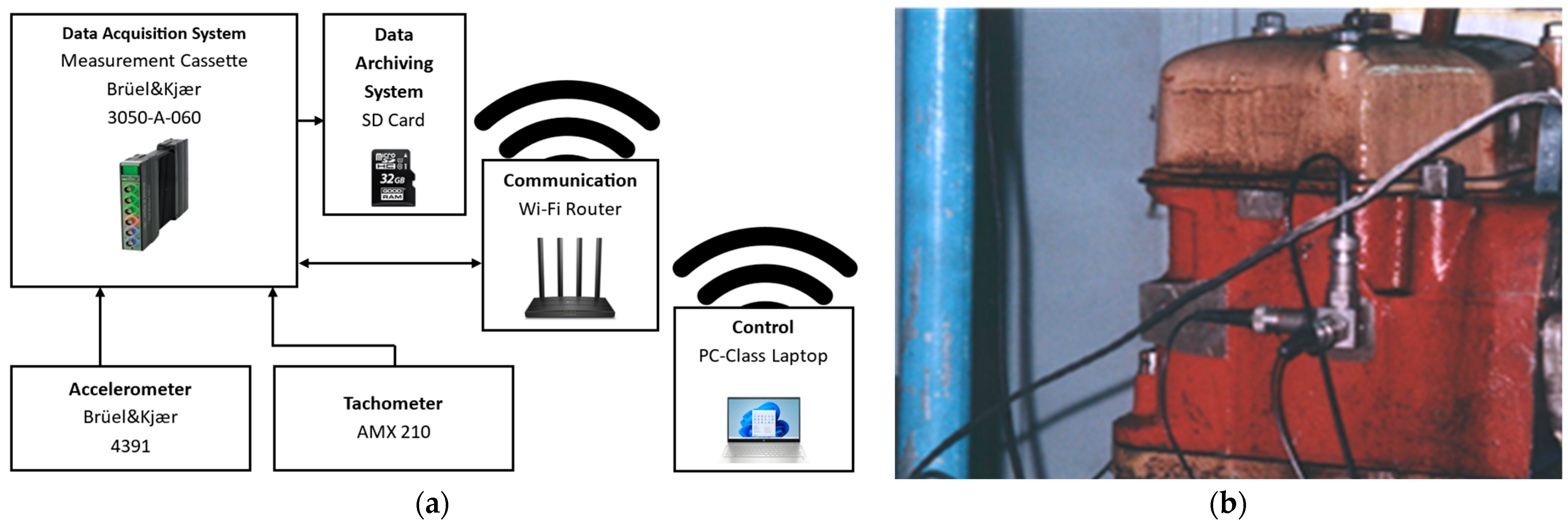
2. Experimental Setup and Data Acquisition

The research was conducted on a single-cylinder research engine type SB 3.1, constructed based on the technical solutions of the multicylinder SW 680 engine. The engine’s design includes a connecting rod, a piston with rings, a cylinder liner, timing valves, a valve control system, an injector, and a modified cylinder head directly derived from the SW 680 engine. This solution provides extensive capabilities for analysing the combustion process and selected operational parameters characteristic of the SW 680 engine series. The SB 3.1 engine enables cylinder pressure measurement, compression ratio (ε) adjustment in the range from 14 to 20, and smooth variation of fuel injection timing and valve timing phases, making it a versatile research stand. The input parameters adopted were combustion pressure and rotational speed. Engine parameters are presented in the table (

Table 1. Parameters of the SB 3.1 engine.

Parameter	Value
Ignition type	Compression ignition
Working cycle	Four-stroke
Maximum useful power (Ne)	23.2 kW at 2200 rpm
Maximum torque (Mo)	109.8 Nm at 1600 rpm
Cylinder bore diameter (D)	0.127 m
Piston stroke (S)	0.146 m
Compression ratio (ε)	15.75
Connecting rod to crank radius ratio (r/L)	0.262
Engine displacement (Vss)	1.852 × 10−3 m3
Number of cylinders (i)	1
Combustion system	Direct fuel injection into the cylinder
Injection pump type	Inline plunger, type P 51T2–10.03 II RVO
Number of valves per cylinder	2
Intake valve opening	4° CA BTDC
Intake valve closing	57° CA ABDC
Exhaust valve opening	42° CA BBDC
Exhaust valve closing	24° CA ATDC
Injector type	W1B-01 with D1LMK 140/2 nozzle
Injector opening pressure	17.5 ± 0.5 MPa

).

To evaluate combustion quality based on vibration signals and operational parameters, the engine was mounted on a dynamometer stand equipped with the following elements:

• AMX 210 eddy-current brake for torque measurement;
• AMX 210 photoelectric sensor for rotational speed measurement;
• AVL 733 gravimetric meter for hourly fuel consumption recording;
• AVL 553 temperature stabilization system to maintain a constant cooling fluid temperature at 75 °C.

The stand was also equipped with a vibration measurement system, comprising a Brüel&Kjær type 4391 piezoelectric transducers mounted on the engine head (tri-axial adapter), a Brüel&Kjær 3050-A-060 measurement cassette (Brüel & Kjær, Nærum, Denmark), and an AVL 364 crankshaft angle marker for synchronization with the engine’s operational cycle. A schematic diagram of the system is presented in Figure 1a. and the vibration signal acquisition location in Figure 1b.

During the tests, the signals were recorded within a frequency band ranging from 0.1 Hz to 10 kHz, with a sampling frequency of 12 kHz, thus enabling spectral analysis up to 6 kHz (in accordance with Nyquist’s criterion). Calibration of the measurement channel was carried out before each measurement series to minimize errors. Controlled quantities were torque (measured and set using the eddy-current brake) and crankshaft rotational speed. The maximum achievable torque on the stand was 90 Nm; thus, five load levels were applied: 0%, 22.5 Nm (25%), 45 Nm (50%), 67.5 Nm (75%), and 90 Nm (100% of maximum torque). The range of rotational speeds included values of 700, 1000, 1200, 1500, and 1700 rpm. At the lowest speed (700 rpm), measurements were conducted exclusively at idle (0% load), since in practical diesel engine operation, significant loads are rarely applied at such low speeds (

Table 2. Engine operating conditions variations.

	Load [Nm]
	0	22.5	45.0	67.5	90.0
Rotational speed [rpm]	700	1000, 1200, 1500, 1700

).

The following output parameters were recorded during the experiments:

• Vibration accelerations of the cylinder head in three orthogonal directions (X, Y, Z);
• Combustion chamber pressure (to assess combustion processes and engine operational correctness);
• Hourly fuel consumption (measured using AVL 733 m).

After completing each measurement series, the data were transferred from the measurement cassette to a computer for subsequent vibration signal analysis.

3. Deep Learning Architecture and Signal Reconstruction

3.1. Dataset

The dataset comprises vibration measurements along the x, y, and z axes, accompanied by pressure readings (considering overpressure relative to atmospheric pressure). Each signal was segmented using a sliding window approach into input arrays of shape (10,000 samples, three channels) with a 50% overlap (5000 samples). The data were partitioned into training (70%), validation (15%), and test (15%) sets, resulting in 4495 training, 963 validation, and 964 testing examples. It should be noted that data splitting was performed before window sampling to avoid data leak. Two preprocessing techniques were applied to the input data:

• Min-Max Scaling: normalizes data to a [0, 1] range;
• Standardization: transforms data to have zero mean and unit variance.

Corresponding pressure outputs were scaled using parameters derived from the training set and applied consistently across validation and test sets with the vibration and pressure signals processed independently for all of the sets. The expected output of the model, corresponding to the pressure values, was also available in the normalized and standardized versions using maximal, minimal, standard deviation, and mean values extracted from the training set and later applied to validation and test sets. The task of the tested models was to produce an output for the whole signal—10,000 floating point numbers representing the pressure of the engine based on the measured x, y, z vibrations—meaning that the three channels with 10,000 floating point measurements were mapped by the model to the 10,000 floating point values representing the pressure (signal-to-signal processing task). To allow for an extensive comparison of the architectures, several models based on commonly utilized architectures were used: autoencoder (AE) [20], U-net [21], Generative Adversarial Network (GAN) [22], and a novel smoothing network (SmM) setup. Furthermore, all models were trained on both the normalized and standardized data to allow for further comparisons. The brief overview of implementations is as follows:

Autoencoder:

• Implemented in two sizes: small (17,121 parameters) and large (188,193 parameters);
• Tested with ReLU and Sigmoid activation functions at the output layer;
• ReLU was considered for data without a fixed upper bound, while Sigmoid was suited for normalized data within [0, 1].

U-Net:

• Adapted for 1D signal processing;
• Two configurations: small (2,046,545 parameters) and large (16,992,849 parameters);
• Tested with both ReLU and Sigmoid output activations.

Generative Adversarial Network:

• Generators based on U-Net architectures with ReLU activation;
• Discriminator implemented as a CNN, classifying inputs as real or fake;
• Loss functions included the following:

  ○

  Discriminator Loss (Binary Cross-Entropy);

  ○

  Weighted combinations of Discriminator Loss with MAE or MSE (weights: 0.6 for Discriminator Loss, 0.4 for MAE/MSE) [23].

Smoothing Models:

• Post-processing model for removing output from the earlier-tested models;
• Dense, convolutional neural network (CNN) [24], U-Net, and Autoencoder architectures were tested;
• Trained on Binary-Cross Entropy and MSE losses;
• Tested with Sigmoid and ReLU output activations.

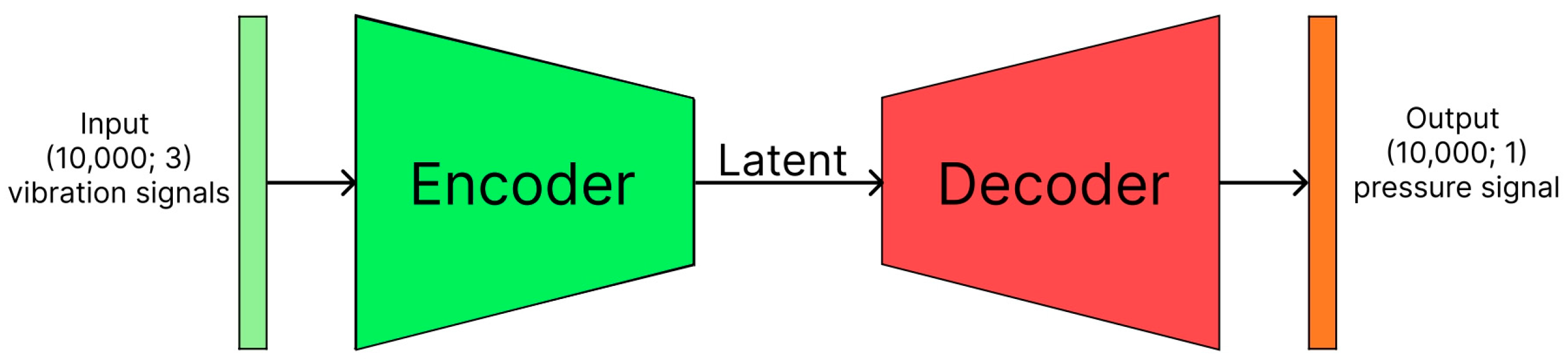
3.2. Autoencoder

The AE models were implemented in several variants; the first two versions can be distinguished based on the size of the model, with the small version (17,121 parameters) and the big version (188,193 parameters). Both models were then implemented in one of two versions, with the last activation function of ReLU and Sigmoid. That was conducted since ReLU might perform better for data with no specified upper bound. Figure 2 shows the general diagram of the autoencoder network used during the experiments.

In contrast, for the data in the range between 0 and 1, Sigmoid might be more beneficial since the model output will be restricted to the expected range of values, producing more natural representations.

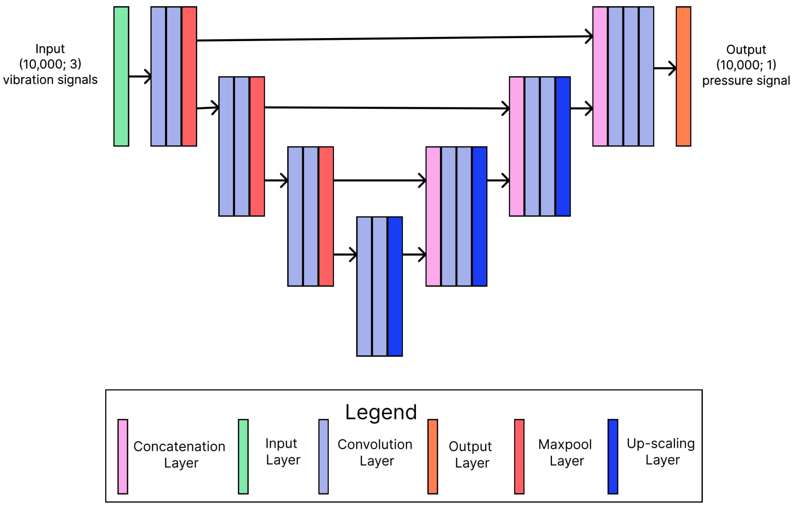
3.3. U-Net

Similarly, the U-net architecture was implemented in the small (2,046,545 parameters) and big (16,992,849 parameters) versions and with both Sigmoid and ReLU activation output functions. For all of these models, the loss was a mean squared error (MSE) [23], and each model was trained for 100 epochs with a batch size of 32 and an early stopping callback after five epochs if no improvement of the MSE on the validation set was observed. The diagram showing the simplified architecture of one of the tested U-net models is shown in Figure 3.

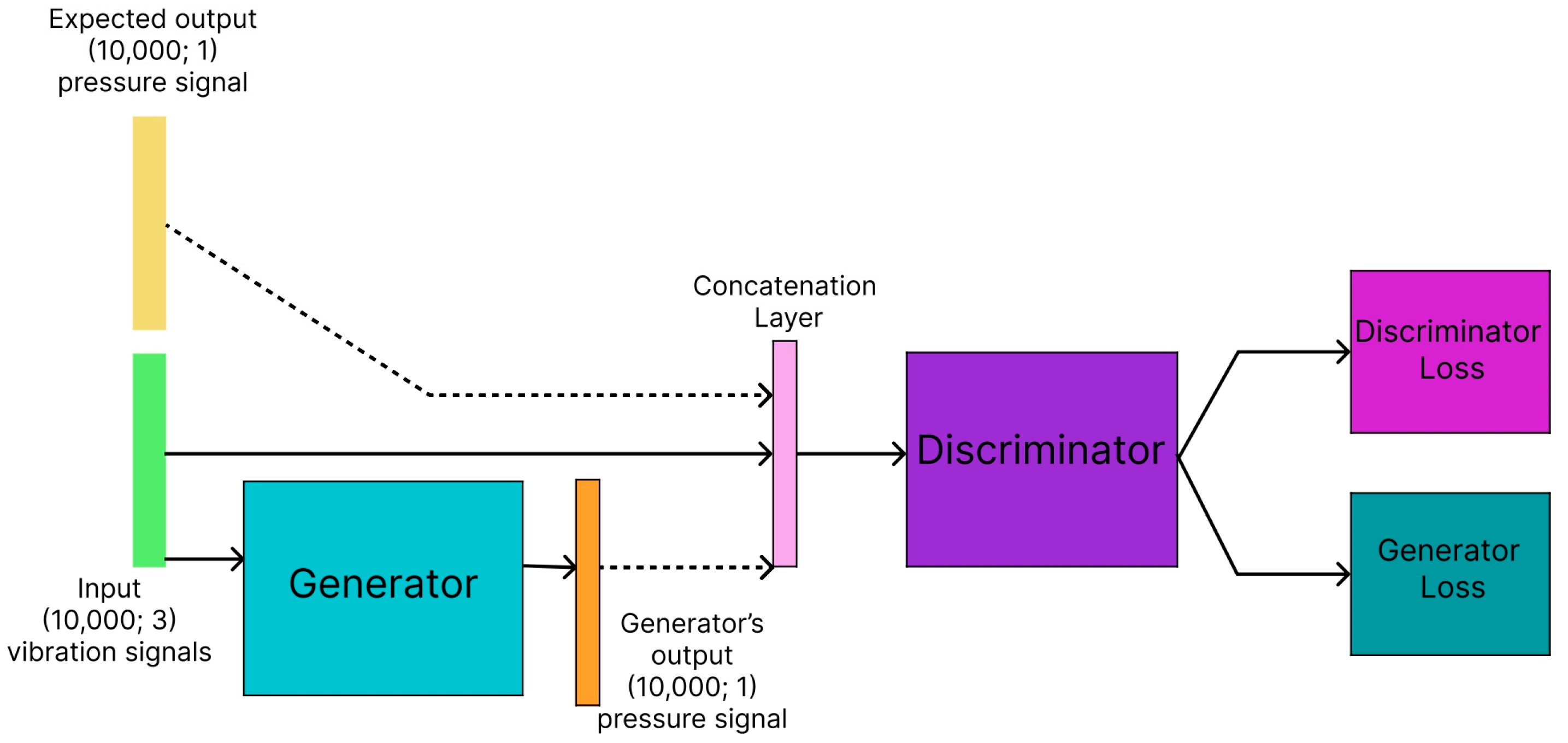
3.4. Generative Adversarial Network

More complicated loss functions than discussed previously were utilized in the implementations of the GAN model. The proposed GAN architectures included two possible generator implementations, based on the U-net architectures with the ReLU activation functions. This architecture was chosen due to its better performance over the AE and U-net, with Sigmoid architectures during the tests of the initial models. The discriminator model was a convolutional neural network (CNN) [24] that functioned as a classifier classifying the training example as real or fake based on the provided x, y, and z vibrations, and the output of the generator model; the output of the discriminator then became a loss function for the generator, forcing the generator to adjust its output so that the discriminator cannot differentiate between real and generated pressure signals. The idea behind utilizing the GAN architecture was to allow the model to discover intricate dependencies to “fool” the discriminator, which might not be possible with relatively simplistic loss functions like MSE and MAE [23]. The diagram representing the idea behind the GAN architecture used in the experiments is presented in Figure 4.

Furthermore, the discriminator model could also be utilized for the detection of anomalies and sensor damage, causing signal distortion. This implicit classification ability is granted by the unique architecture. However, to further enrich the information produced by the loss function in the GAN models, a weighted mean between MAE and the discriminator’s output was utilized in one scenario, and the weighted mean between MSE and the discriminator’s output was utilized in another version of the model. In such a case, the discriminator’s output was multiplied by 0.6, and the MAE/MSE loss was multiplied by 0.4. It is important to note that the training of GAN models takes longer than for the previously mentioned models with a loss based only on the MSE. Additionally, GAN models tend to get stuck in local optima due to the discriminator having a much easier task than the generator. However, methods exist to combat this phenomenon, such as label smoothing [25] or the Wasserstein GAN models [26], though they are not the focus of this work.

Table 3. A general summary of the models used in the experiments, which were trained to reconstruct the engine’s pressure signal based on the input vibration signal.

Model	Parameters	Loss Functions	Activation Functions
Autoencoder–small	17,121	MSE	ReLU/Sigmoid
Autoencoder–big	188,193
U-Net–small	2,046,545
U-Net–big	16,992,849
GAN-Generator (U-net–small)	2,046,545	1—Discriminator Loss; weighted Sum between 1—Discriminator Loss; and MAE/MSE	ReLU
GAN-Generator (U-net–big)	16,992,849	1—Discriminator Loss; weighted Sum between 1—Discriminator Loss; and MAE/MSE	ReLU
GAN-discriminator	2,586,897	BCE	Sigmoid

shows the tested models used for the task of recreating the pressure signal of the engine based on the input x, y, z vibration signal. Each model was trained on min–max scaled and standardized data without the post-processing smoothing model.

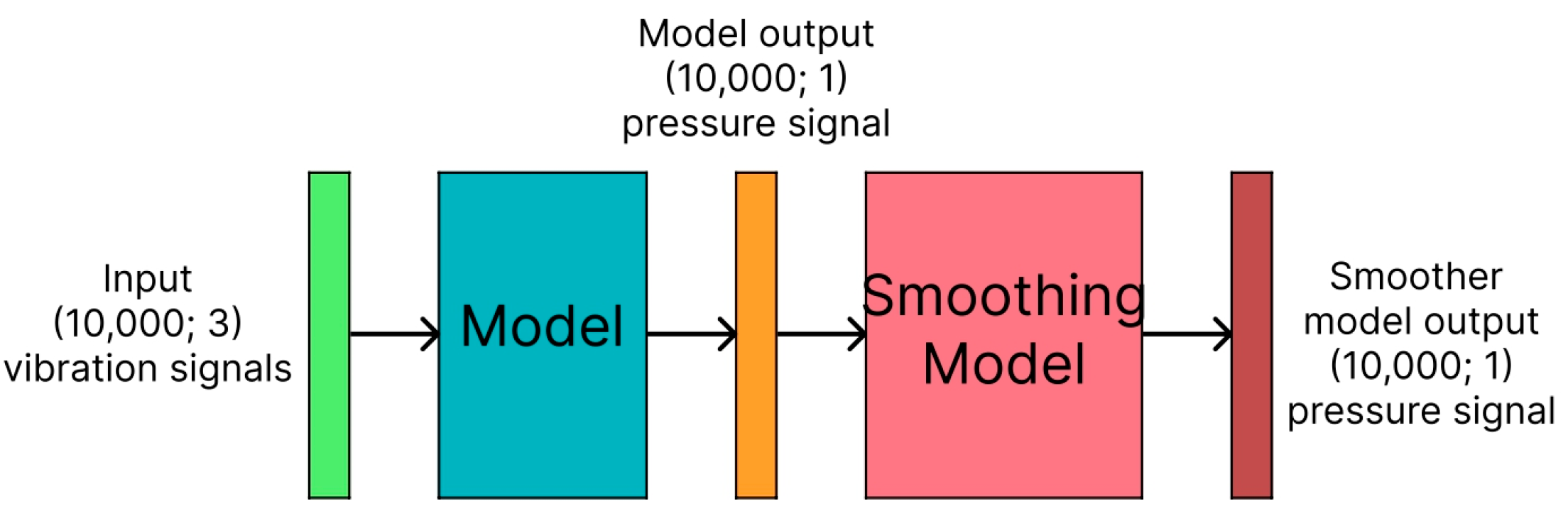
During the experiments, it was observed that the results produced by all the models tested thus far suffered from the problem of producing unexpected spikes in the output where none were expected. However, such produced values seemed to have values lower than the correctly identified spikes by the model. As such, this has led to the idea of creating an additional model that would work on the output of the originally trained model to smooth out and get rid of the noisy and unwanted spikes in the recreated signal. These models will be referred to as “smoothing models” (SmNs). A SmN was given as input, the output of an already trained model, which was meant to produce the pressure signal, and the expected output of the SmN model would be the corrected signal without false spikes or noise. The SmN should learn what kinds of errors are produced by the original model and correct them. For each of the previously trained models, nine different smoothing models were trained. The architecture of three of these models was based on the ANN with dense layers, The remaining models were based on the CNN architecture, with two AE models and two U-net models.

Furthermore, the models were trained twice, using Binary Cross-Entropy (BCE) and MSE loss. The most important part of the mapping from vibrations to pressure signals is the correct detection of pressure spikes. As such, utilizing the BCE loss can allow the model to treat the task as a binary classification task to find spikes as positive classes and no spikes as negative classes. Figure 5 shows the idea behind utilizing the smoothing model on another model’s output.

Table 4. Smoothing models.

Model	Parameters	Loss Functions	Activation Functions
Convolutional Model–Small	945	MSE/BCE	ReLU
Simple Dense ANN	170,960	MSE/BCE	ReLU/Sigmoid
Convolutional Model	724,225
U-net	65,729
Autoencoder	2,046,497

shows the tested smoothing models. Each model shown in the table was trained based on the output of every model shown in Table 3. A smoothing model is given as input, the pressure signal of the model it was paired with in the training, then the smoothing model aims to output an improved recreation of the pressure signal by removing errors and noise from the signal originally produced by the model.

4. Results

For a comparative assessment of the models, a measure of similarity between the real pressure waveform and the pressure generated by the model was created. The use of an additional measure to evaluate models apart from MSE was necessary because models can achieve relatively low MSE with outputs that are of constant value, since the most common value appearing in the pressure signal is 0. The measure of similarity was defined as the harmonic mean of two values:

$$SM={\displaystyle \frac{2}{\sqrt{\frac{1}{{\rho }_1}+\frac{1}{{\rho }_2}}}},$$

(1)

where ${\rho }_1$ is the correlation coefficient between model and real values of the pressure waveform.

The measure ${\rho }_2$ was defined as a normalized difference in instantaneous pressure values:

$${\rho }_2={\displaystyle \frac{1}{N}}\sum _{\mathrm{i}=1}^N{\displaystyle \frac{\left|r_{\mathrm{i}}-m_{\mathrm{i}}\right|}{max\left(r\right)}}$$

(2)

where r_i is the real value of the pressure, m_i is the reconstructed pressure value, N is the number of samples, and max(r) is the maximum value of the entire signal.

The first component of measure (1) is easy to interpret and contains information about the linear relationship between the reproduced and model waveforms but does not contain information about the difference between the pressure values generated by the model and the real ones. Hence, it is necessary to use both components. The measure was tested on many simulated waveforms and performed well in assessing waveform similarity. It is important to note that this similarity measure (SM) was (directly in model building) not used directly in model building due to potential computational complexity, which would not allow for a timely comparison of such a vast quantity of models. It was applied for a comparative assessment of the obtained results generated using different models.

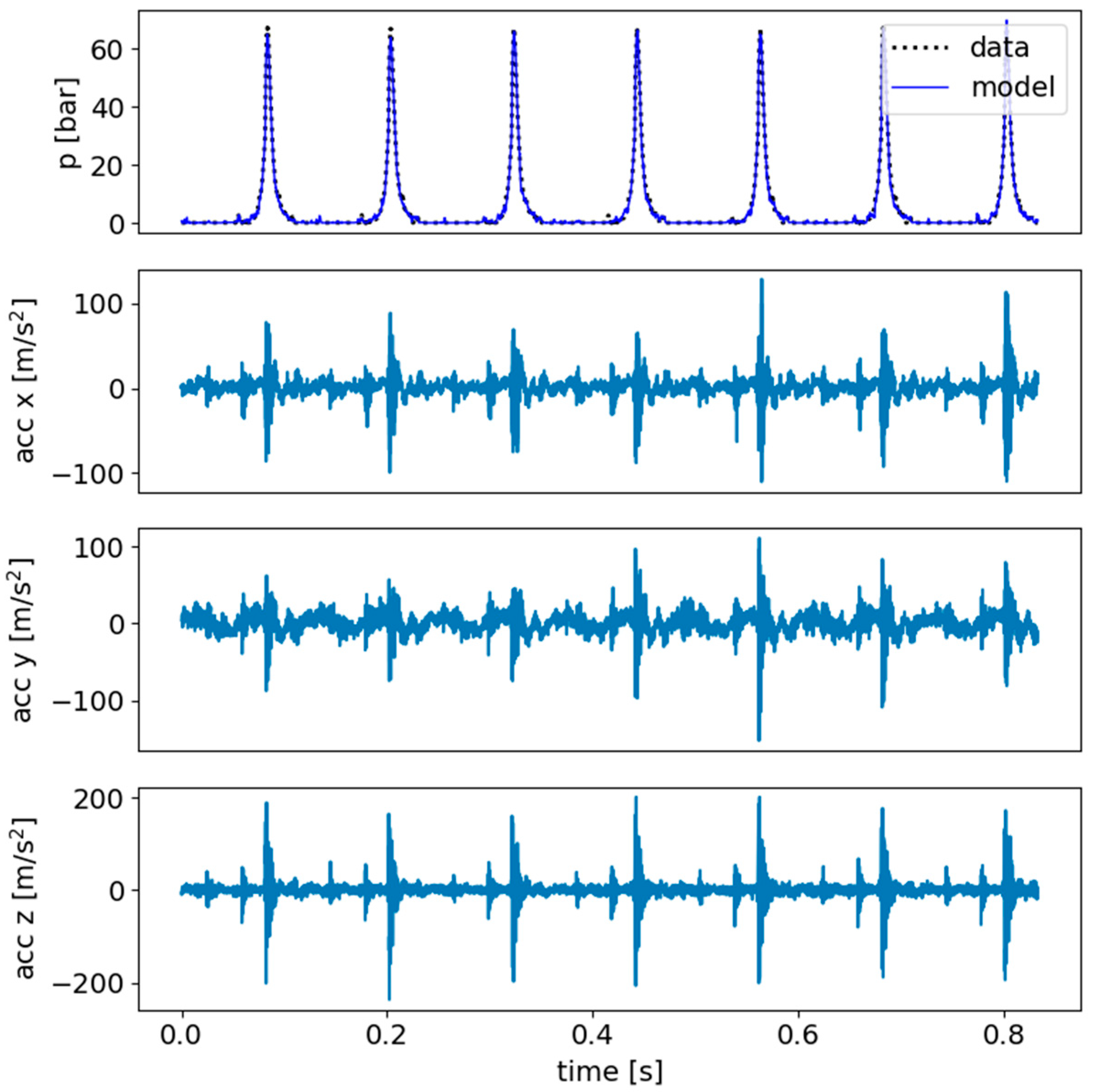
The best-performing model was the U-net model with an ReLU output activation function, with the output being smoothed by another U-net model and the BCE loss applied in the training of the smoothing model. The model has managed to achieve a value of 0.993 using the aforementioned similarity measure for both validation and test sets. The results of the model’s prediction of the engine’s pressure are visible in Figure 6.

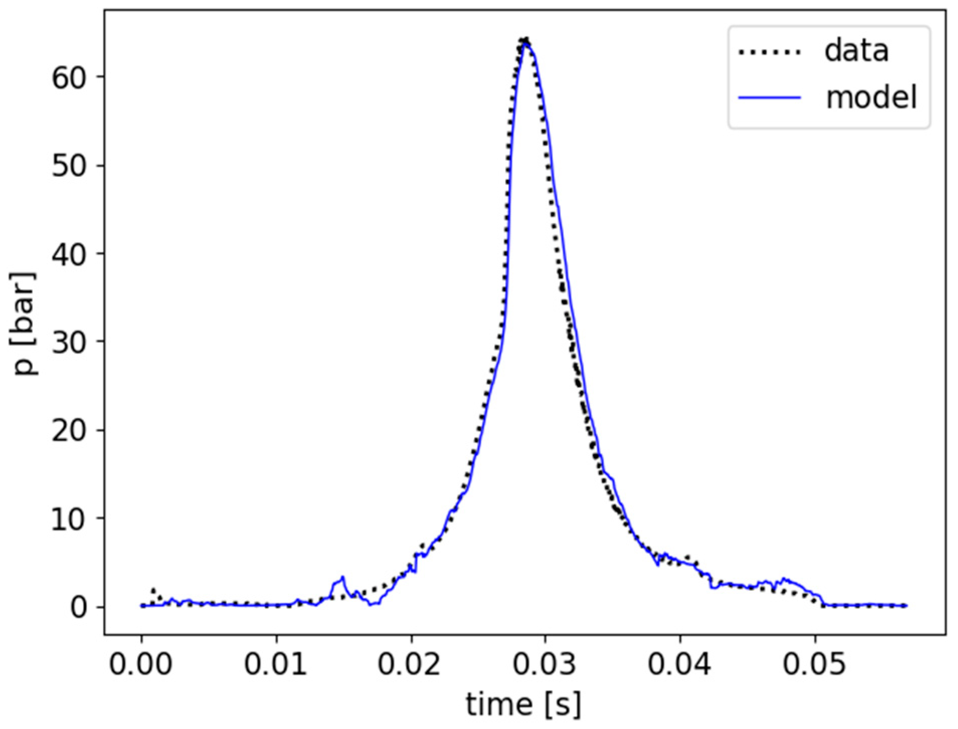
To generate the final pressure curve for a given rotational speed and load, the reconstructed pressure curves were averaged. Figure 7 presents a comparison of the averaged expected output and the averaged reconstructed output for the best-performing model for a random example from the validation set.

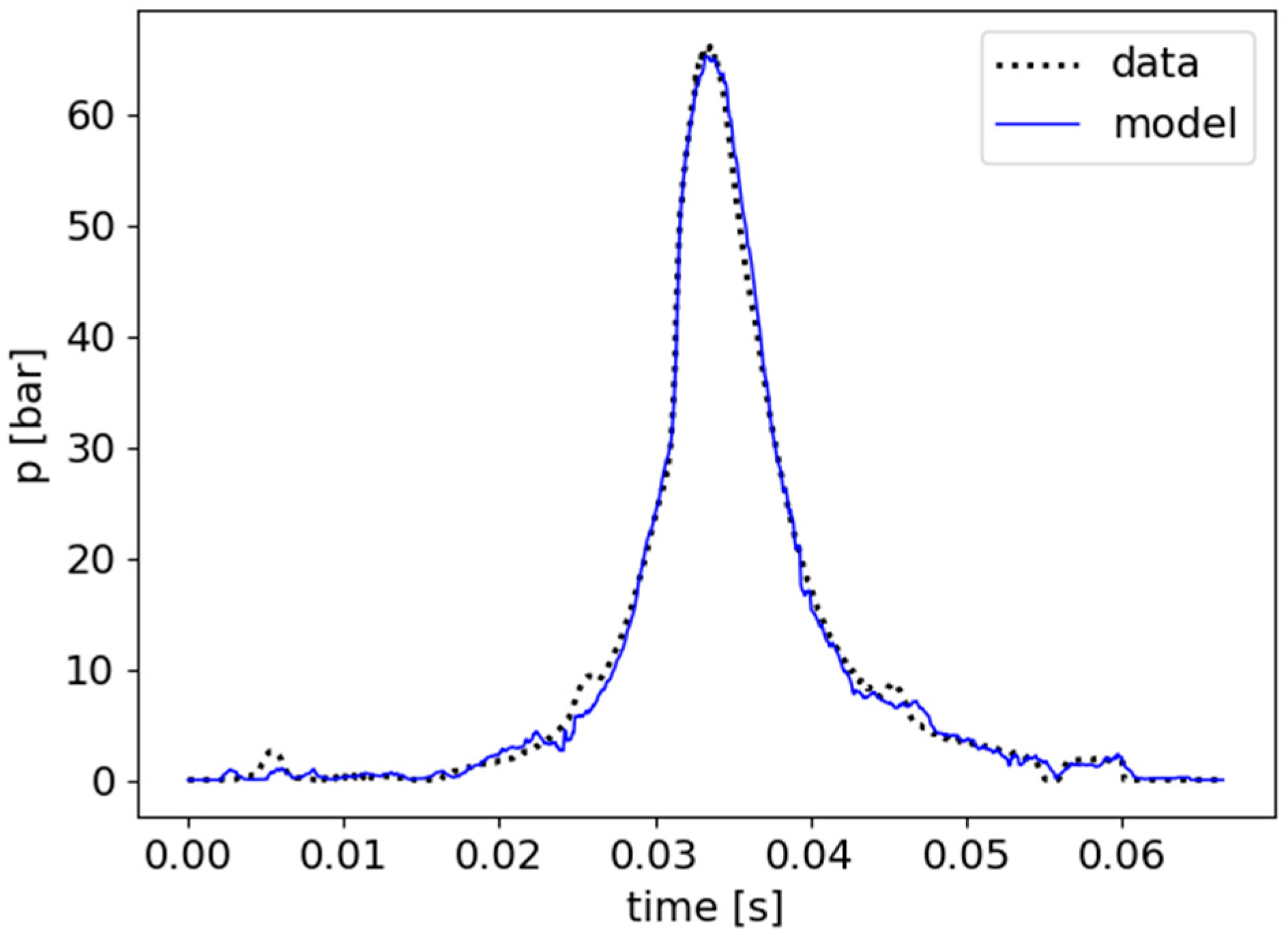
Furthermore, the performance of the model does not seem to differ for previously unseen examples, as the model still manages to achieve a very high similarity score of 0.993 for the test set. To further showcase the model’s performance for unseen data, Figure 8 was included, which shows a comparison of the expected pressure values of the engine and the model’s output after averaging and centring the values for a random example from the test set.

The conducted experiments also showcase that even the largest models exceeding 16 million parameters can be efficiently deployed on modern CPUs with the inference time of the model measured at 1.2541 s, suggesting that even relatively larger models could be utilized for real-time inference, even though the architecture should be used for maintenance checks that do not necessarily need to be run in real-time.

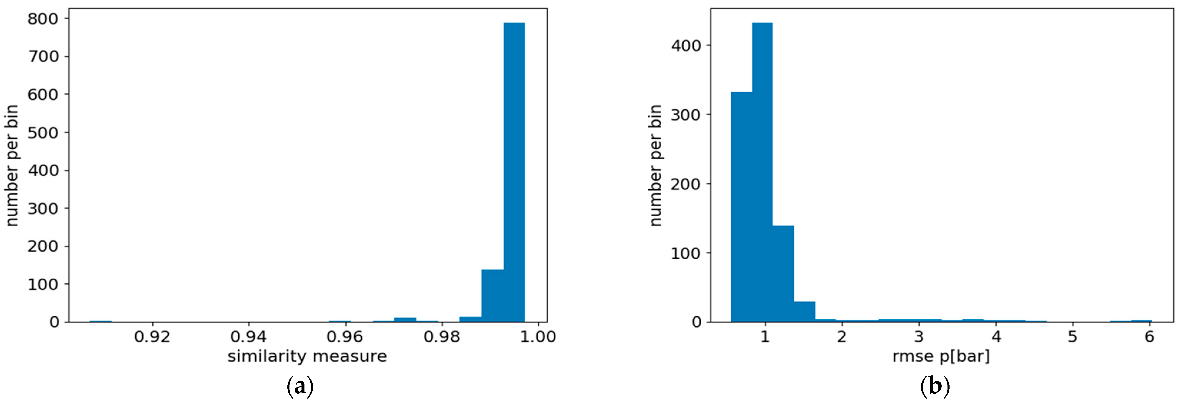
Lastly, the presented Figure 9 shows the histogram of all values of the similarity measure (Figure 9a) and root mean squared error (Figure 9b) for the test set for the best-performing model.

As the presented results show, the best model reconstructs the pressure waveforms with high accuracy for all available data, enabling high reliability of diagnostic inferences. Furthermore, the analysis of the results has shown that of the four best-performing models, three of them used the smoothing model; as such, it seems that the addition of the smoothing model is a good choice for the signal-to-signal processing task using ANNs.

Table 5. The four best-performing models for recreating internal engine pressure based on vibration signals, with values provided for the test set.

Model	Activation Functions	Smoothing Model	Smoothing Model Output Activation Function	Smoothing Model Loss Function	Similarity Measure for the Test Set
U-net–small	ReLU	U-net	ReLU	BCE	0.9935
U-net–small	ReLU	U-net	ReLU	MSE	0.9929
U-net–small	ReLU	U-net	Sigmoid	MSE	0.9920
U-net–big	ReLU	-	-	-	0.9918

shows the comparison of the best-performing models for the described task of recreating internal engine pressure based on the measured x, y, and z vibration signals.

Lastly,

Table 6. Comparison of similarity measures for the best models with various architectures.

Model	Activation Functions	Smoothing Model	Smoothing Model Output Activation Function	Smoothing Model Loss Function	Similarity Measure for the Test Set
U-net–small	ReLU	U-net	ReLU	BCE	0.9935
Autoencoder–small	ReLU	U-net	ReLU	BCE	0.9909
GAN (generator–U-net small)	ReLU	U-net	ReLU	BCE	0.9783
U-net–big	ReLU	-	-	-	0.9918
Autoencoder–small	ReLU	-	-	-	0.9673
GAN (generator– U-net big)	-	-	-	-	0.9232

compares the best-performing models for each model architecture for the test set. Based on the results, it can be observed that the U-net architecture adapted to the 1d signal-to-signal task achieves better results than the remaining Autoencoder and GAN models, when paired with the smoothing model. Additionally, the GAN architecture can also produce surprisingly good results if the generator architecture is based on the U-net model. Lastly, the most promising models utilize the novel smoothing architecture for post-processing the model’s original output. The most effective approach combines a U-net model with an additional smoothing model, which also employs the U-net architecture and is trained using the BCE loss function. This combination yields the best results on both validation and testing sets, as demonstrated by the similarity function.

5. Discussion and Conclusions

The presented study set out to determine whether purely external vibration measurements can be transformed, without any handcrafted features, into high-fidelity reconstructions of in-cylinder pressure. There, well-established signal-to-signal deep-learning architectures (autoencoders, U-Nets, and GANs) were benchmarked. Additionally, a novel two-stage model composed of a “base” U-Net followed by a dedicated smoothing network (SmN) was introduced. The proposed two-stage method for reconstructing the pressure curve in the engine cylinder based on vibration measurements using a smoothing network delivers the best result among the tested models (SM = 0.9935). The reconstruction errors are minimal and insignificant when averaging. The proposed method can serve as a highly effective tool for diagnosing engine damage that affects the pressure curve.

However, several key limitations of the study should be noted, due to the vast number of deep-learning architectures being available, this work was focused on only a small number of those most relevant to the problem. However, several other architectures could be tested, such as recurrent networks utilizing LSTM [27] or GRU [28] layers. Transformer architecture could also be a promising direction for future analysis [29]. Furthermore, only the steady-state performance of a single engine was tested; to propose a more universal tool a more robust analysis with the aforementioned methodology should be applied to a more varied dataset. Regardless, the potential of the smoothing technique applied to the signal processed by a deep-learning model was demonstrated.

Several other observations can be drawn from this work:

• Importance of architecture depth vs. capacity: Larger networks did not systematically outperform smaller ones once the SmN was introduced; the small U-Net + SmN (~2 M + 66 k parameters) slightly surpassed the 17 M-parameter “big” U-Net. Thus, hierarchical receptive fields matter more than sheer width for this task.
• Role of the similarity function: The custom metric SM (harmonic mean of correlation and normalized amplitude error) proved essential. Pure MSE rewarded flat, low-variance outputs, whereas SM penalised such trivial solutions, causing clear ranking shifts among otherwise comparable models. As such, this measure can be recommended for future pressure-reconstruction work because it balances shape fidelity and amplitude accuracy.
• Effectiveness of the smoothing network: Despite training on the base model’s outputs only, the SmN eliminated ≈ 90 % of spurious micro-spikes and improved the SM by 0.002–0.005 across all backbones. Training the SmN with binary-cross-entropy (interpreting spikes as the positive class) delivered the best generalisation, suggesting that the residual error is dominated by misclassified peak events rather than continuous noise.
• GANs vs. deterministic losses: GAN generators delivered visually plausible signals, but their stochastic training produced higher variance and occasional mode collapse, reflected in lower worst-case SM. As such, coupling the model with SmN may be necessary if implemented in practice.

In summary, deep-learning-based vibration-to-pressure translation augmented by a lightweight smoothing stage offers a powerful new diagnostic tool that can bring cylinder-pressure insights to any engine where mounting pressure sensors is impractical or uneconomical. However, future research could further explore the domain adaptation to other engine types, adapting the post-processing SmN architecture to more difficult tasks, such as analysis of multiple output signals from different models, or focus on embedding the discriminator of the GAN as an online anomaly detector for sensor faults. The limitations of applying such a method and its effectiveness were not the focus of this study and may require further research. Furthermore, exploration of online-learning techniques could be beneficial in cases where signals can be subject to change due to external factors other than cylinder pressure.