Development of a Discrete Algorithm for Interpreting Ground-Penetrating Radar Data in Vertically Heterogeneous Media

Abstract

This study presents the development of a discrete algorithm for interpreting ground-penetrating radar (GPR) data in vertically inhomogeneous media for the diagnostics of road structures. Experimental data were obtained using an OKO-2 GPR system, followed by primary radargram processing using the CartScan software. This included noise and interference filtering, as well as the initial estimation of the dielectric permittivity of detected layers. The resulting dataset was used to validate numerical algorithms for solving the forward and inverse problems of geolectrics. The proposed approach is based on minimizing a quadratic misfit functional between the calculated and observed values of the horizontal component of the electromagnetic field. The gradient of the functional required for optimization is obtained via the numerical solution of an adjoint problem. A discrete version of this problem was developed, which satisfies the properties of conservativeness and uniformity according to finite difference theory. The inverse problem reconstruction of dielectric permittivity is considered a non-destructive method for radargram interpretation. Assuming a piecewise-continuous medium structure eliminates the need for computing gradients at material interfaces. The proposed methodology enhances the accuracy and reliability of pavement condition assessment and holds practical value for road infrastructure monitoring.

1. Introduction

GPR has become a crucial tool in various fields of natural sciences and engineering [1]. The GPR method is characterized by high resolution and versatility, which has led to its widespread application in various scientific, technological, and practical fields. It is actively used in engineering surveys, archaeological research, geological and geophysical studies, road monitoring tasks, and experimental applications [2,3,4,5].

• In construction: quality control of concrete structures, detection of reinforcing elements, and assessment of foundation conditions [6,7];
• In geology and geophysics: stratigraphic mapping, detection of karst voids, and analysis of moisture content and rock structure [8,9];
• In road diagnostics: identification of voids, structural defects, waterlogged areas, and disruptions in the layered structure [10,11,12];
• In archaeology: non-destructive probing of cultural layers, determination of building locations, and identification of burial sites [13,14,15].

Additionally, in geological studies, GPR is widely used to investigate active faults without resorting to invasive ground-based methods. Its applications include determining optimal trench locations for paleoseismological studies [16] and characterizing the shallow-depth geometry of active fault systems using both 2D and 3D datasets of GPR data [17].

The primary tool for GPR research is a device that emits electromagnetic pulses into a subsurface medium as it moves along the surface. The OKO-2 series [8] is widely used due to its suitability for non-destructive testing, being specifically designed for non-destructive testing of engineering structures, assessment of road surface conditions, and performance of geotechnical investigations.

The OKO-2 complexes feature a modular architecture, which allows for the rapid replacement of antennas operating at frequencies of 400 MHz and 1000 MHz [18]. The 400 MHz antenna configuration offers an optimal trade-off between penetration depth (up to 2–3 m) and spatial resolution (approximately 10 cm), making it particularly effective for the examination of road structures.

The signals reflected from the boundary between media are recorded by the receiving antenna, converted into electrical impulses, and stored as a time-domain scan, commonly referred to as a radar image. Each point in the radar profile corresponds to the signal travel time, enabling the reconstruction of the internal structure of the investigated subsurface medium.

One of the key tasks in GPR data analysis is the interpretation of radar profiles focused on reconstructing the subsurface structure. In other words, the goal is to determine the geoelectric cross-section of the investigated object based on the recorded electromagnetic response. The development of effective interpretation methods is essential for improving diagnostic accuracy, enhancing the reliability of conclusions, and expanding the application of GPR as a key method in non-destructive testing.

Traditional interpretation methods rely on engineering algorithms integrated into the software of GPR systems.

An alternative approach focuses on the rigorous mathematical formulation and resolution of coefficient-based inverse problems in electrodynamics. Such methods are designed to reconstruct the spatial distribution of physical properties, such as the dielectric permittivity, by analyzing recorded data regarding the propagation of electromagnetic waves at observation points.

The works of Iskakov and Kabanikhin [19,20], as well as the study [21], have made a significant contribution to the development of theoretical methods for interpreting radargrams. These contributions focus on the construction of optimization algorithms for solving inverse coefficient problems in geoelectrics, particularly in layered and vertically inhomogeneous media, along with establishing the correctness and stability of the obtained solutions. These investigations have laid the foundation for modern high-precision and adaptive algorithms for processing GPR data, which are especially valuable for assessing complex engineering and geological structures and detecting subsurface defects.

The theoretical foundations and numerical methods for addressing inverse problems in geoelectrics, including proofs of the existence and uniqueness of solutions, are comprehensively detailed in the monograph by Romanov and Kabanikhin [22]. This work serves as a cornerstone for subsequent research in the field of geophysical inversion problems.

A comparison of different methods for solving various inverse coefficient problems is presented in the work of the authors [23].

A number of studies [24,25] have devoted significant attention to the preprocessing of GPR data with the goal of enhancing interpretation quality. Specifically, various noise suppression techniques are employed, including wavelet transformations (e.g., fourth-order Haar and Daubechies wavelets), frequency filtering, sliding averaging, amplitude correction, Butterworth filters, and Levinson–Durbin algorithms. Additionally, Fourier transforms are specifically utilized to extract the key characteristics of the electromagnetic wave field.

A key area of research involves the development of numerical algorithms for solving the inverse problem at the discrete level. In other words, this approach yields a difference scheme with the property of conservation, ensuring energy conservation at the discrete level. The effectiveness of this approach is demonstrated in the studies by Rysbayula et al. [26,27] and in the work by Karchevsky [28], where a comparative analysis of traditional and discrete approaches is conducted based on numerical examples.

In contrast to existing approaches, the proposed discrete algorithm conserves fundamental physical principles, is specifically tailored for vertically inhomogeneous media, and ensures numerical stability.

Modern research in geoelectrics highlights the growing adoption of machine learning methods for automating data analysis and enhancing geophysical interpretation. One promising area is the application of unsupervised learning, such as clustering (e.g., the K-Means algorithm), for comprehensive analysis of geoelectric tomography data. In [29], an approach was proposed for identifying areas of filtrate contamination with high reliability and minimal interpretative subjectivity based on resistivity, chargeability, and their ratio.

In addition, deep learning methods have been actively applied in flaw detection tasks, such as in the analysis of GPR data. In [30], a study presents an algorithm designed for the automatic detection of hidden defects beneath the lining of railway tunnels using a modified YOLOP architecture. This approach demonstrated high performance, achieving up to 80.6% accuracy with a processing time of less than 0.02 s per image.

The integration of geophysical methods with machine learning algorithms enables automation, enhances result reliability, and minimizes expert reliance on complex engineering and geological tasks.

This study examines algorithms for GPR sensing based on numerical modeling of the propagation of electromagnetic waves in inhomogeneous media governed by Maxwell’s equations. The inverse problem is formulated as the reconstruction of the geoelectric structure, namely, the determination of the spatial distribution of the medium’s physical properties based on the recorded response data. In the context of electromagnetic geophysics, the key information is provided by the horizontal component of the electric field vector measured at the observation point.

The numerical algorithms developed in this paper address both the direct and adjoint problems in a discrete form. Moreover, the adjoint problem preserves key physical properties of the model, including energy conservation at the discrete level, thereby enhancing the reliability of the derived results.

To enhance the reliability of interpretation, preprocessing of experimental data is essential for isolating informative signals and suppressing noise [25].

The measurement component of the GPR system facilitates the recording of reflected waves, implements automatic time-varying gain control, performs gating, and conducts signal digitization. Gating is performed by the control and synchronization unit. One radar trace is generated through the emission and recording of 512 pulses. Sequential recording of all traces along the profile generates the final radar image.

The processing of GPR data comprises the following key steps [25]:

• data acquisition and validation;
• spectral analysis of direct and reflected waves;
• sliding-window summation to mitigate common-mode noise;
• frequency-domain filtering to suppress interference components;
• amplitude correction to account for signal attenuation;
• static corrections accounting for topographic variations;
• spatial interpolation of data along the profile;
• velocity analysis of common-midpoint gathers;
• signal migration to enhance the spatial resolution of detected objects.

Based on the theoretical and applied aspects discussed above, the primary objectives of this study are as follows:

• development of algorithms for the primary processing of GPR data;
• solution of direct and inverse problems for subsurface radar;
• implementation of discrete analogs for optimization methods.

2. Materials and Methods

As noted above, solving the inverse coefficient problem requires GPR data, which serves as additional time-domain information. Therefore, this subsection presents experimental results and outlines the steps for processing the acquired signals.

2.1. Algorithms for the Primary Processing of GPR Data

As part of this research project, experimental studies were conducted using the OKO-2 series GPR (GEOTECH company, Moscow, Russia). A 400 MHz central frequency antenna was used for probing, providing an optimal balance between penetration depth and resolution. Measurements were performed with a sampling frequency of 1 GHz, an antenna separation of 0.3 m, and a scanning step of 0.15 m along the survey line.

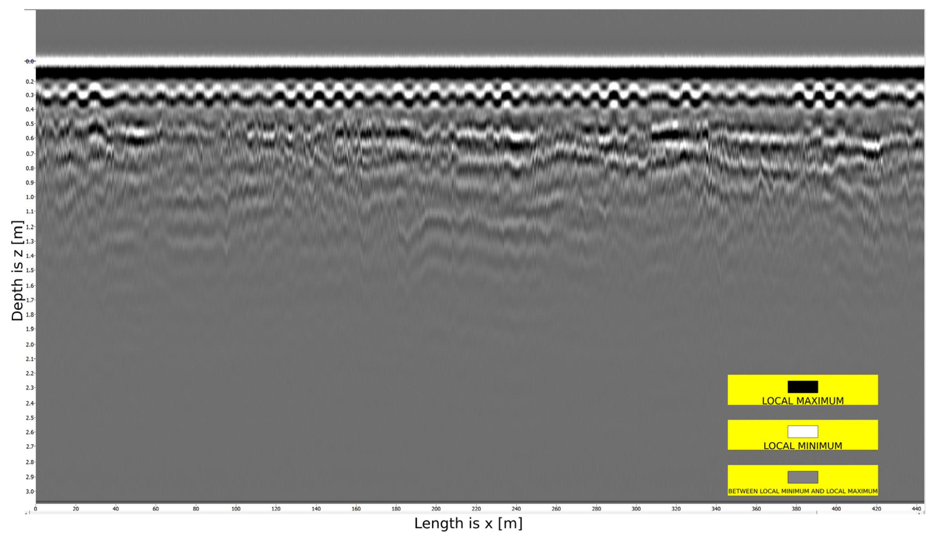
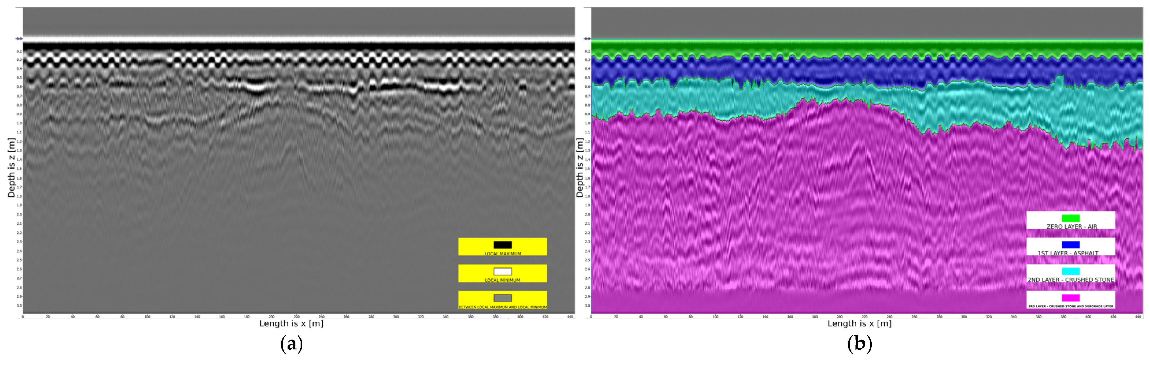
The algorithm for primary data processing was implemented using the specialized CartScan software [31] (GEOTECH company, Moscow, Russia) supplied with the GPR equipment. The main objectives of the processing were to suppress low-frequency noise, eliminate external interference, and enhance reflected signals corresponding to the boundaries of the road pavement layers. Figure 1 presents the raw profile of a 500-meter-long radar image acquired without signal amplification.

Figure 1 shows the subsurface structure, where the vertical axis ($Oz$) indicates the depth within the pavement structure (with a maximum signal penetration depth of 3 m), and the horizontal axis ($Ox$) represents the length of the surveyed road segment (with a maximum length of 500 m). The image also displays black, white, and gray shades. Black areas correspond to local signal maxima, white to minima, and gray to intermediate values.

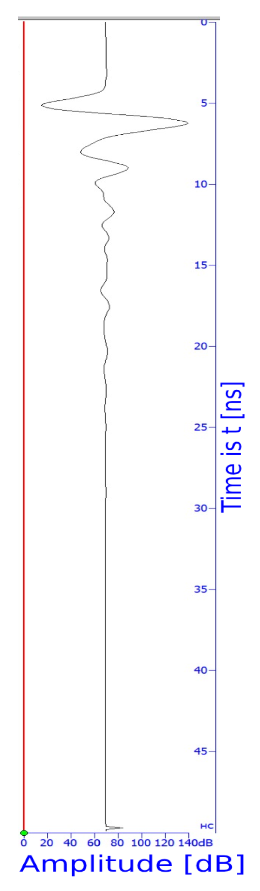
Drawing a vertical line from any point $x_0$ of the radar profile (Figure 1) along the $Ox$-axis yields a 2D graph, as shown in Figure 2.

The 2D graph depicted in Figure 2 is referred to as a trace. The trace represents a time-dependent function (the medium’s response), illustrating the behavior of an electromagnetic pulse as it propagates through the subsurface medium. Here, the absolute value of the function corresponds to the signal amplitude.

The distance between adjacent traces along the Ox-axis is 15 cm. The collection of all traces forms the radar profile (Figure 1). Given that the length of the road in the radar profile is 500 m, the number of traces in the profile is approximately 3333.

Since the signal has a central frequency of 400 MHz, it exhibits minimal sensitivity to noise and interference. Therefore, bandpass filtering, intended to remove noise and interference, is unnecessary.

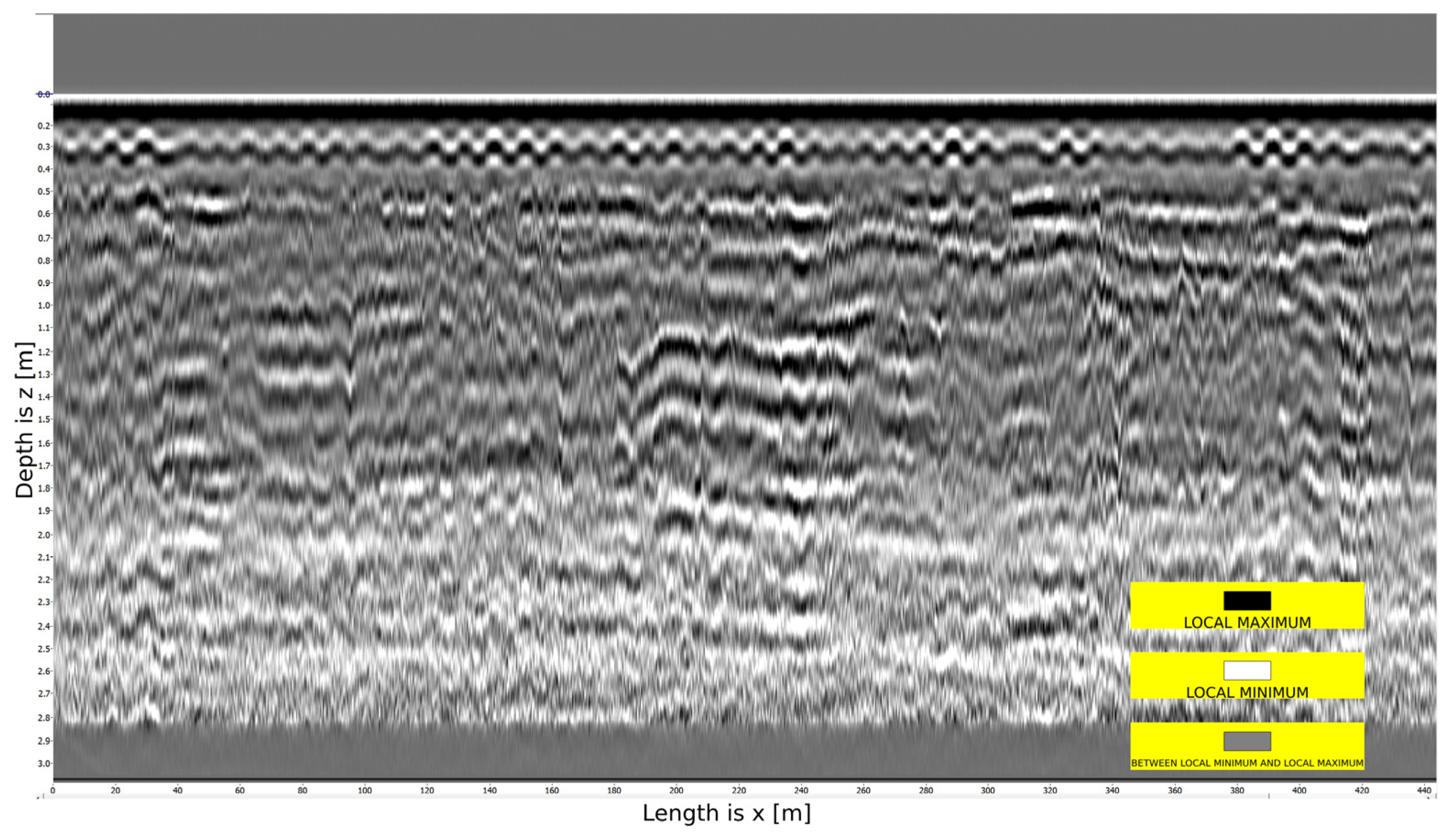
The next step involves applying mean subtraction (Figure 3), which entails calculating the average trace across all traces in the profile and subtracting it from each trace.

The subsequent step involves applying automatic gain control (AGC) (Figure 4) to enhance the visibility of the signal at greater depths, accounting for the attenuation of the signal amplitude with depth.

AGC represents an algorithm utilized in data processing systems, including mobile applications for road diagnostics, such as the CartScan software package [31]. The primary purpose of AGC is to maintain a stable input signal level through dynamic gain adjustment. This is particularly critical when analyzing vehicle vibrations, as it enables compensation for variations in driving conditions, vehicle types, and smartphone mounting configurations.

The algorithm evaluates the power or amplitude of the accelerometer signal, compares it with a reference level, and adjusts the gain to maintain the signal within the optimal range. This enhances the system’s sensitivity to minor road surface defects and improves the quality of subsequent analysis, including the identification of potholes and surface irregularities.

AGC is also widely employed in other fields, such as global satellite navigation systems (GNSS), where its performance may be compromised by intentional interference, including high-power interference signals (jamming) or signal spoofing [32]. In such cases, signal characteristics may be altered, leading AGC to produce inaccurate estimations, thereby impacting the overall system performance. Modern research focuses on modeling the behavior of AGC under interference conditions and developing methods to enhance its robustness.

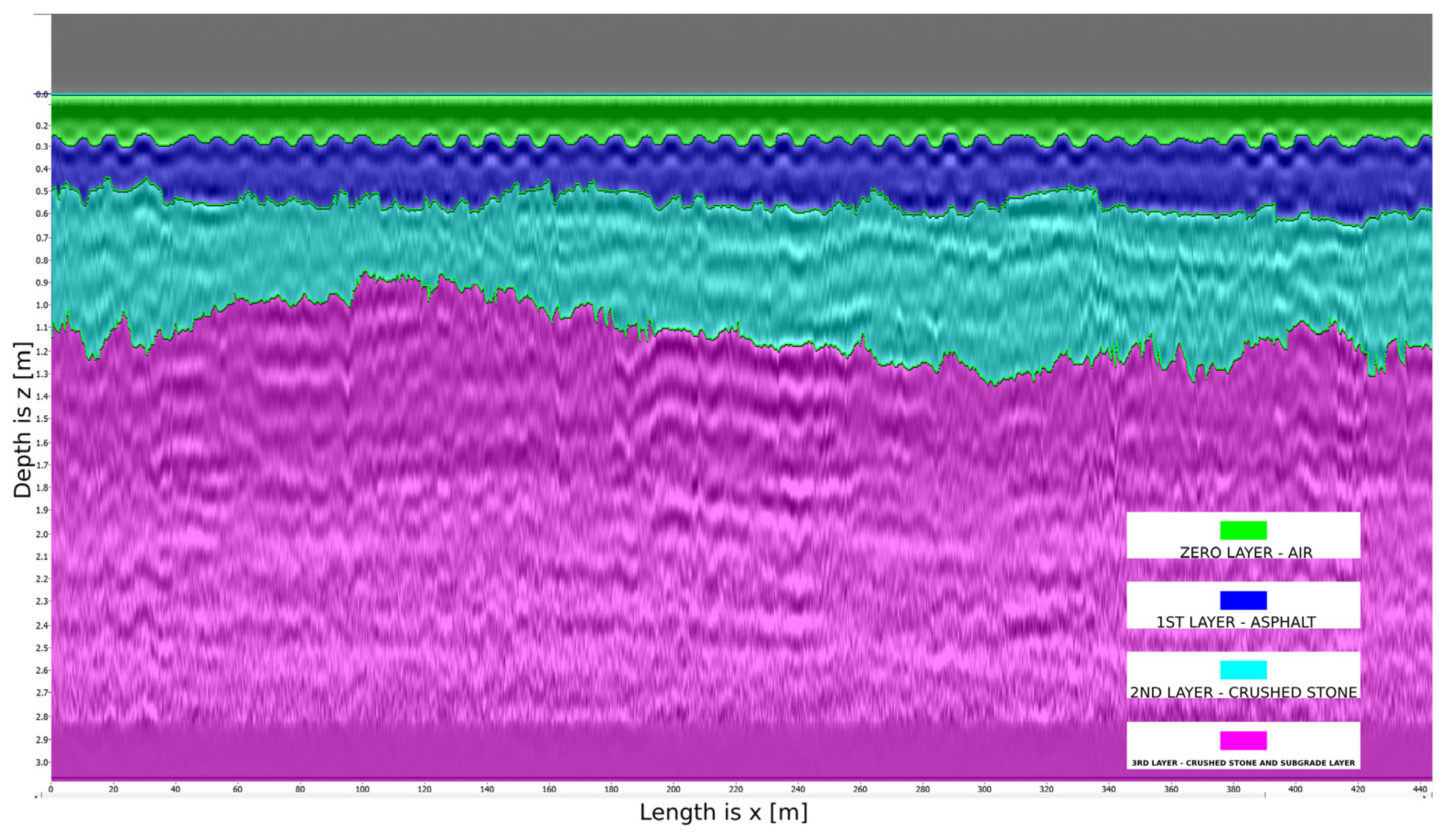
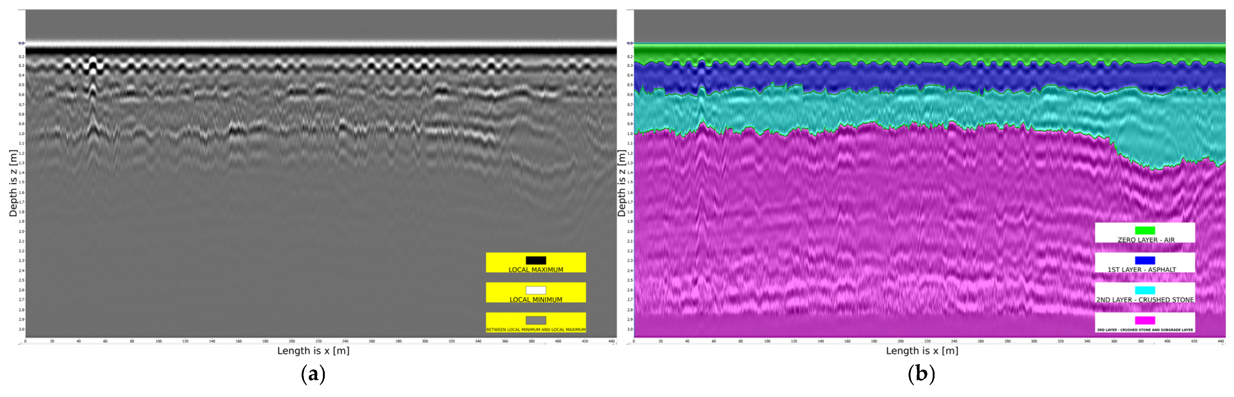
The next step is the delineation of road surface layer boundaries, as illustrated in Figure 5.

For further details on layer boundary selection, refer to [31]. The layer boundaries were identified based on the white color, corresponding to local minima. The boundaries of only three layers were successfully delineated, ranging from the blue layer to the pink layer, with the green layer representing air. The boundary between the third and fourth layers remains indistinguishable due to signal attenuation.

Profiles are classified into two types based on the morphology of the layer boundaries:

• An acceptable profile refers to a georadar section in which the reflected layer boundaries exhibit a relatively uniform and horizontal shape, lacking pronounced anomalies. Such boundaries correspond to the proper construction of road structures in compliance with regulatory standards for layer thickness and density;
• A problematic profile is characterized by localized irregularities such as bulges or concavities in the reflective boundaries, which may indicate substrate heterogeneity, the presence of defects (e.g., binder leaching, subsidence, or voids), or non-compliance with construction technology.

Subsidence typically occurs when the underlying layer exhibits high moisture content or due to the presence of groundwater. Concavities can also form when accumulated moisture in the underground structure freezes during winter.

The main acceptance criteria include

• the stable shape of the reflective boundaries, free from distortions and displacements exceeding 10–15% of the average layer thickness;
• the absence of local signal amplification and attenuation;
• compliance of the layer geometry with design documentation or typical pavement structure specifications.

We will examine examples of both acceptable and problematic profiles. Figure 6 illustrates a problematic profile where the boundary of a concave layer is evident.

Figure 7 presents another problematic profile, characterized by the boundary of a convex layer, while Figure 8 demonstrates an acceptable profile.

It is important to note that, by default, the CartScan software assigns a relative dielectric permittivity of 5 to each layer in Figure 5. Consequently, the depth values along the $Oz$-axis for the layer boundaries in Figure 5, Figure 6, Figure 7 and Figure 8 exhibit inaccuracies. However, the a priori thickness of each layer can be manually adjusted, allowing for corrections to the layer thickness in the radar image profiles.

According to road pavement standards, the top layer consists of fine-aggregate asphalt with a thickness of 0.07 m. This is followed by a coarse-aggregate asphalt concrete layer with a thickness of 0.08 m. Beneath these layers are crushed stone layers: one with a grain size of 4 mm and a thickness of 0.3 m and another with a grain size of 8 mm and a thickness of 0.25 m. Finally, the subgrade layer consists of natural soil.

The dielectric permittivity of each layer can be estimated based on its thickness. This approach, which determines the dielectric permittivity using layer thickness, is referred to as the engineering method.

To ensure the reliability of profile data over a 500-meter length, core sampling must be performed at a specific location $x_0$ along the highway to verify the accuracy of the data regarding the thickness of each pavement layer. Additionally, in future research, experiments involving sample extraction will be performed to acquire accurate data on layer thickness and dielectric permittivity for each stratum.

2.2. Formulation of the Direct and Inverse Problems of GPR

For a more rigorous description of signal propagation in an inhomogeneous medium, the forward and inverse problems of GPR are formulated. The forward problem simulates the behavior of the electromagnetic field given known parameters, while the inverse problem focuses on recovering unknown parameters of the subsurface medium, which is crucial for the subsequent interpretation of GPR data.

The physical formulation of a GPR problem is as follows: an external current source $j^{ex}$ is activated on the asphalt surface, which has a bell-shaped temporal profile $r\left(t\right)$. Simultaneously, the electromagnetic field (the medium’s response) is measured on the asphalt surface over a duration of approximately 50 nanoseconds. The measurement duration depends on the frequency of the electromagnetic pulse; for instance, it is approximately 50 ns for 400 MHz and 16 ns for 1000 MHz. Based on these measurements, it is required to determine the properties of the medium (dielectric permittivity $\epsilon$, electrical conductivity $\sigma$) at depths ranging from zero to 2.2 m.

Consider a problem in which the parameters $\epsilon$ and $\sigma$ depend on depth $z$, and the external current source is modeled as a cable of considerable length, positioned centrally and aligned along the roadway (along the $Oz$-axis). In this scenario, neglecting the influence of the cable’s ends and the lateral boundaries of the road, we arrive at the following Cauchy problem for the $E_2$ component of the electric field vector [22]:

$$\mathit{\epsilon }{\displaystyle \frac{{\partial }^2}{{\partial t}^2}}{E}_2+\sigma {\displaystyle \frac{\partial }{\partial t}}{E}_2={\displaystyle \frac{1}{\mu }}{∆}_{xz}{E}_2-w\left(x\right)v\left(z\right)r’\left(t\right),$$

(1)

$${\left.E_2\right|}_{t=0}=0, {\displaystyle \frac{\partial }{\partial t}}{\left.E_2\right|}_{t=0}=0,$$

(2)

Here, $\mathit{\epsilon }={\mathit{\epsilon }}_0{\mathit{\epsilon }}_r$, ${\mathit{\epsilon }}_0=8.854·{10}^{-12}$ [F/m], $\mu ={\mu }_0{\mu }_r$, ${\mu }_0=1.257·{10}^{-6}$ [H/m], $w\left(x\right),$ and $v\left(z\right)$ are functions describing the spatial extent of the source.

To study the direct problem (1)–(2), we choose a vertically heterogeneous medium model. Based on the standard road model, we consider a four-layer medium. At the media boundaries, we adopt the average geophysical characteristics of the layers. Thus, the horizontal dotted lines $z^1=0.15$ m, $z^2=0.45$ m, $z^3=0.7$ m, and $z^4=2.2$ m correspond to the boundaries between homogeneous layers (these values are derived from pavement standards). In each layer, the values of ${\mathit{\epsilon }}_r$ and $\sigma$ are constant.

For subsequent calculations, we consider a vertically inhomogeneous medium model in which the geophysical properties are averaged at the layer boundaries, which is consistent with practical observations.

We formulate a one-dimensional approximation of problem (1)–(2). We apply the Fourier transform operator with respect to the variable $x$ and rewrite (1)–(2) as [22]:

$$\epsilon U_{tt}+\sigma U_t={\displaystyle \frac{1}{\mu }}\left(U_{zz}-{\lambda }^{2}U\right)-W_{\lambda }v\left(z\right)r^{\prime }\left(t\right),$$

(3)

$${\left.U\right|}_{t=0}=0, {\left.U_t\right|}_{t=0}=0,$$

(4)

where $U=F_x\left[E_2\left(x,z,t\right)\right]$; $W_{\lambda }=F_x\left[w\left(x\right)\right]$, and $\lambda$ is the Fourier transform parameter in $x$.

Statement of the Direct Problem: Given the piecewise constant functions $\epsilon \left(z\right)$ and $\sigma \left(z\right)$, as well as the positive constant $\mu$, determine the function $U$ as the solution to the generalized Cauchy problem defined by Equations (3) and (4).

Additional Information: Suppose additional information is available regarding the solution of the direct problem (3)–(4) at $z=0$, representing the medium’s response:

$$U^{\lambda }\left(0,t\right)=f\left(t\right).$$

(5)

Formulation of the Inverse Problem: Given $\sigma \left(z\right), \mu$ and the additional information (5) (with $\lambda ={\lambda }_0$ fixed), determine $\epsilon \left(z\right)$ and $U^{{\lambda }_0}$ from Equations (3) and (4).

2.3. Discrete Analogs of Optimization Methods

For the practical implementation of inverse problem-solving methods, it is necessary to transition from continuous mathematical models to their discrete analogs. This transition is driven by the requirements of numerical stability, computational accuracy, and the need for algorithmic implementation. Accordingly, discrete schemes for solving direct and adjoint problems have been developed, which exhibit the required properties of conservation and stability.

To perform numerical calculations, we limit the analysis to the finite domain $Q=\left[0,T\right]\times \left[0,L\right]$.

We consider the inverse boundary value problem in the wave formulation, where the goal is to determine the approximate value of $\epsilon$. The governing equations are as follows:

$$\mu p{U}_{tt}+\mu \sigma U_t=U_{zz}-{\lambda }^{2}U,$$

(6)

$${\left.U\right|}_{t=0}=0, {\left.U_t\right|}_{t=0}=0,$$

(7)

$${\left.U_z\right|}_{z=0}=\mu g\left(t\right), {\left.U\right|}_{z=L}=0,$$

(8)

Here, $p\left(z\right)$ is an approximate solution to the inverse problem, and the function $g\left(t\right)$ is a Gaussian pulse with parameter $\alpha$:

$$g\left(t\right)={\displaystyle \frac{\alpha }{\sqrt{\pi }}}{e}^{-{\left(\alpha t\right)}^2}.$$

(9)

The quadratic functional is defined as

$$J\left[p^{\left(n\right)}\right]={\int }_0^T{\left[U\left(0,t;p^{\left(n\right)}\right)-f\left(t\right)\right]}^{2}dt, n=0, 1,\hspace{0.33em}2, \dots .\hspace{0.33em}$$

(10)

The gradient of the functional is given by

$$𝛻J\left[p^{\left(n\right)}\right]=\mu {\int }_0^T{U}_{tt}\left(z,t;p^{\left(n\right)}\right)\cdot \psi \left(z,t;p^{\left(n\right)}\right)dt,\hspace{1em}n=0, 1,\hspace{0.33em}2,\hspace{0.33em}\dots .$$

(11)

Adjoint problem:

$$\mu p{\psi }_{tt}-\mu \sigma {\psi }_t={\psi }_{zz}-{\lambda }^2\psi ,$$

(12)

$${\left.\psi \right|}_{t=T}=0, {\left.{\psi }_t\right|}_{t=0}=0,$$

(13)

$${\left.{\psi }_z\right|}_{z=0}=2\left[U\left(0,t;p\right)-f\left(t\right)\right], {\left.\psi \right|}_{z=L}=0,$$

(14)

The derivation of formulas (11) for calculating the gradient and the corresponding adjoint problem (12)–(14) is provided in [22].

The conjugate gradient optimization method [22]:

$$p^{(n+1)}=p^{\left(n\right)}-{\gamma }_n{s}_n, n=0, 1, 2, \dots .$$

(15)

where the parameters ${\gamma }_n$ and $s_n$ are calculated as follows:

$${\gamma }_n={\displaystyle \frac{J\left[p^{\left(n\right)}\right]}{{‖𝛻J\left[p^{\left(n\right)}\right]‖}^2}}, n=0, 1, 2, \dots ,$$

(16)

$$s_0=𝛻J\left[p^{\left(0\right)}\right], s_n=𝛻J\left[p^{\left(n\right)}\right]-{\beta }_n{s}_{n-1}, n=1, 2, \dots .$$

(17)

The parameter ${\beta }_n$ is calculated using the following formula:

$${\beta }_n=-{\displaystyle \frac{{‖𝛻J\left[p^{\left(n\right)}\right]‖}^2}{{‖𝛻J\left[p^{\left(n-1\right)}\right]‖}^2}}, n=1, 2, \dots .$$

(18)

The stopping condition for the optimization method (15)-(18) is given by

$$‖𝛻J\left[p^{\left(n-1\right)}\right]‖<\delta , \forall \delta >0, n=1, 2, \dots .$$

(19)

As the parameter $\delta$ decreases, the number of iterations $n$ increases, leading to a longer execution time for the iterative method and also improving the accuracy of the solution.

The convergence of the optimization method described by Equations (15)–(19) has been proven in [33].

To discretize the formulas of the direct (6)–(8) and adjoint (12)–(14) problems, we employ implicit difference schemes [34], which are unconditionally stable. The explicit scheme requires adherence to the Courant condition.

We derive formulas for the direct (6)–(8) and adjoint (12)–(14) problems at the discrete level. To achieve this, we proceed as follows:

(a)

The domain of continuous variation in the arguments $Q=\left[0,T\right]\times \left[0,L\right]$ is discretized into a grid as follows:

$${\Omega }_{\tau h}=\left\{\left(i\hspace{0.33em}h,\hspace{0.33em}{t}_k\right),\hspace{0.33em}i=\overline{0,N},\hspace{0.33em}k=\overline{0,M},\hspace{0.33em}h=L/N,\hspace{0.33em}{\tau }_k=t_k-t_{k-1}, k=\overline{1,M}, {\overline{\tau }}_k=\left({\tau }_k+{\tau }_{k-1}\right)/2, k=\overline{2,M}\right\}.$$

(20)

A non-uniform grid with respect to $t$ is computed as follows [19]:

$$t\left(q\right)=\left\{\begin{array}{c} {\displaystyle \frac{C\eta q}{\xi -q}},\hspace{1em}\hspace{1em}\hspace{1em}\hspace{1em}\hspace{1em}\hspace{1em}\hspace{1em}\hspace{1em}0\le q\le q_0,\\ {\displaystyle \frac{\left(T-C{\eta }^{1-\beta }\right)\left(q-1\right)}{1-q_0}}+T,\hspace{1em}\hspace{1em}\hspace{1em} q_0\le q\le 1,\hfill \end{array}\right.$$

(21)

where $0<\beta \le 0.5$, $0<C<1$, $\xi =q_0\left(1+{\eta }^{\beta }\right)$, $\eta =1/{\alpha }^2$.

The direct problem (6)–(8) is approximated by an implicit difference scheme [34]:

$${\displaystyle \frac{\mu p_i}{{\overline{\tau }}_k}}\left({\displaystyle \frac{y_i^{k+1}-y_i^k}{{\tau }_{k+1}}}-{\displaystyle \frac{y_i^k-y_i^{k-1}}{{\tau }_k}}\right)+\mu {\sigma }_i{\displaystyle \frac{y_i^{k+1}-y_i^{k-1}}{{2\overline{\tau }}_k}}={\displaystyle \frac{y_{i+1}^{k+1}-y_i^{k+1}+y_{i-1}^{k+1}}{h^2}}-{\lambda }^2{y}_i^{k+1}, i=\overline{1,N-1}, k=\overline{1,M-1},$$

(22)

$$y_i^0=0, y_i^1=0, y_N^k=0, i=\overline{1,N-1}, k=\overline{2,M},$$

(23)

$$y_1^{k+1}=y_0^{k+1}+h{g}^{k+1}+{\displaystyle \frac{h^2}{2}}\left({\displaystyle \frac{\mu p_0}{{\overline{\tau }}_k}}\left({\displaystyle \frac{y_0^{k+1}-y_0^k}{{\tau }_{k+1}}}-{\displaystyle \frac{y_0^k-y_0^{k-1}}{{\tau }_k}}\right)+\mu q_0{\displaystyle \frac{y_0^{k+1}-y_0^{k-1}}{{2\overline{\tau }}_k}}+{\lambda }^2{y}_0^{k+1}\right), k=\overline{1,M-1}$$

(24)

Additional information:

$$y_0^k\left\{p_i\right\}=f^k,\hspace{0.33em}\hspace{0.33em}k=\overline{2,M}.$$

(25)

The adjoint problem (12)–(14) is also approximated using an implicit difference scheme [34]:

$${\displaystyle \frac{\mu p_i}{{\overline{\tau }}_k}}\left({\displaystyle \frac{{\phi }_i^{k+1}-{\phi }_i^k}{{\tau }_{k+1}}}-{\displaystyle \frac{{\phi }_i^k-{\phi }_i^{k-1}}{{\tau }_k}}\right)-\mu {\sigma }_i{\displaystyle \frac{{\phi }_i^{k+1}-{\phi }_i^{k-1}}{{2\overline{\tau }}_k}}={\displaystyle \frac{{\phi }_{i+1}^{k-1}-{\phi }_i^{k-1}+{\phi }_{i-1}^{k-1}}{h^2}}-{\lambda }^2{\phi }_i^{k-1}, i=\overline{1,N-1}, k=\overline{M-\mathrm{1,1}},$$

(26)

$${\phi }_i^M=0, {\phi }_i^{M-1}=0, {\phi }_N^k=0, i=\overline{1,N-1}, k=\overline{M-\mathrm{2,0}}$$

(27)

$${\phi }_1^{k-1}={\phi }_0^{k-1}+h\left[y_0^{k-1}-g^{k-1}\right]+{\displaystyle \frac{h^2}{2}}\left({\displaystyle \frac{\mu p_0}{{\overline{\tau }}_k}}\left({\displaystyle \frac{{\phi }_0^{k+1}-{\phi }_0^k}{{\tau }_{k+1}}}-{\displaystyle \frac{{\phi }_0^k-{\phi }_0^{k-1}}{{\tau }_k}}\right)-\mu {\sigma }_0{\displaystyle \frac{{\phi }_0^{k-1}-{\phi }_0^{k-1}}{{2\overline{\tau }}_k}}+{\lambda }^2{\phi }_0^{k-1}\right), k=\overline{M-\mathrm{1,1}}.$$

(28)

(b)

We consider a discrete analog of the functional (10) and its gradient (11) as follows:

$$J\left[p\right]=\sum _{k=1}^{M-1}{\left[y_0^k\left\{p_i\right\}-f^k\right]}^2{\overline{\tau }}_k,$$

(29)

$$𝛻J\left[p_i\right]=\mu \sum _{k=1}^{M-1}{y}_i^k\{p_i\}\left({\displaystyle \frac{{\phi }_i^{k+1}-{\phi }_i^k}{{\tau }_{k+1}}}-{\displaystyle \frac{{\phi }_i^k-{\phi }_i^{k-1}}{{\tau }_k}}\right), i=\overline{1,N-1}.$$

(30)

These formulas were derived to ensure that the difference schemes preserve the conservative property of energy, namely, the conservation of energy at the discrete level. The derivation of the formulas for the gradient (30), along with the corresponding adjoint problem (26)–(28), has been performed.

To minimize the functional, we employ the conjugate gradient method [22].

3. Results

The developed numerical algorithms were tested using real-world data from pavement structures obtained experimentally. As part of this research project, approximately 2000 km of highways in the Akmola region were investigated using GPR.

During the calculations, the characteristics of reconstructing the dielectric permittivity for various layers of the medium were analyzed. Additionally, the accuracy of the reconstructed parameters was evaluated.

A layered medium model representing the road surface is considered:

• The first layer consists of asphalt (fine- and coarse-grained) with a glass fiber reinforcement interlayer;
• The second layer is a base layer composed of a mixture of fine crushed stone with a grain size of 4 mm and containing 7% cement by weight;
• The third layer is a base layer composed of a mixture of coarse crushed stone with a grain size of 8 mm;
• The fourth layer is the subgrade layer, which is soil (loam).

These data were obtained using the CartScan software package, whose algorithm is described in detail in Section 2.1.

Table 1. Model of the road pavement.

Layer Number	1-st Layer	2-nd Layer	3-rd Layer	Subgrade Layer
${\epsilon }_r$	3.0	6.0	4.0	20.0
$\sigma$ [S/m]	0.00512	0.00725	0.00592	0.0132
$z$ [m]	0.15	0.45	0.7	2.2

${\epsilon }_r$ is relative dielectric permittivity; $\sigma$ is electrical conductivity; $z$ is depth.

illustrates the properties of the medium validated by experts from the Road Asset Quality Center. Since the formulation of the problem (6)–(8) was derived from the system of Maxwell’s equations in the wave formulation, the skin effect occurs as a physical phenomenon. Consequently, the signal can attenuate before reaching the subgrade layer.

We determine the depth at which the skin effect occurs. To achieve this, we use the following formula [28]:

$$H_s=\sqrt{{\displaystyle \frac{2}{\mu {\omega }_0\sigma }}},$$

(31)

where the reference angular frequency ${\omega }_0$ is equal to $\sigma /\epsilon$. To calculate the depth of the skin effect, we consider the dielectric permittivity $\epsilon$ and the electrical conductivity $\sigma$ of the subgrade layer. The result is $H_s=1.27 \mathrm{m}$.

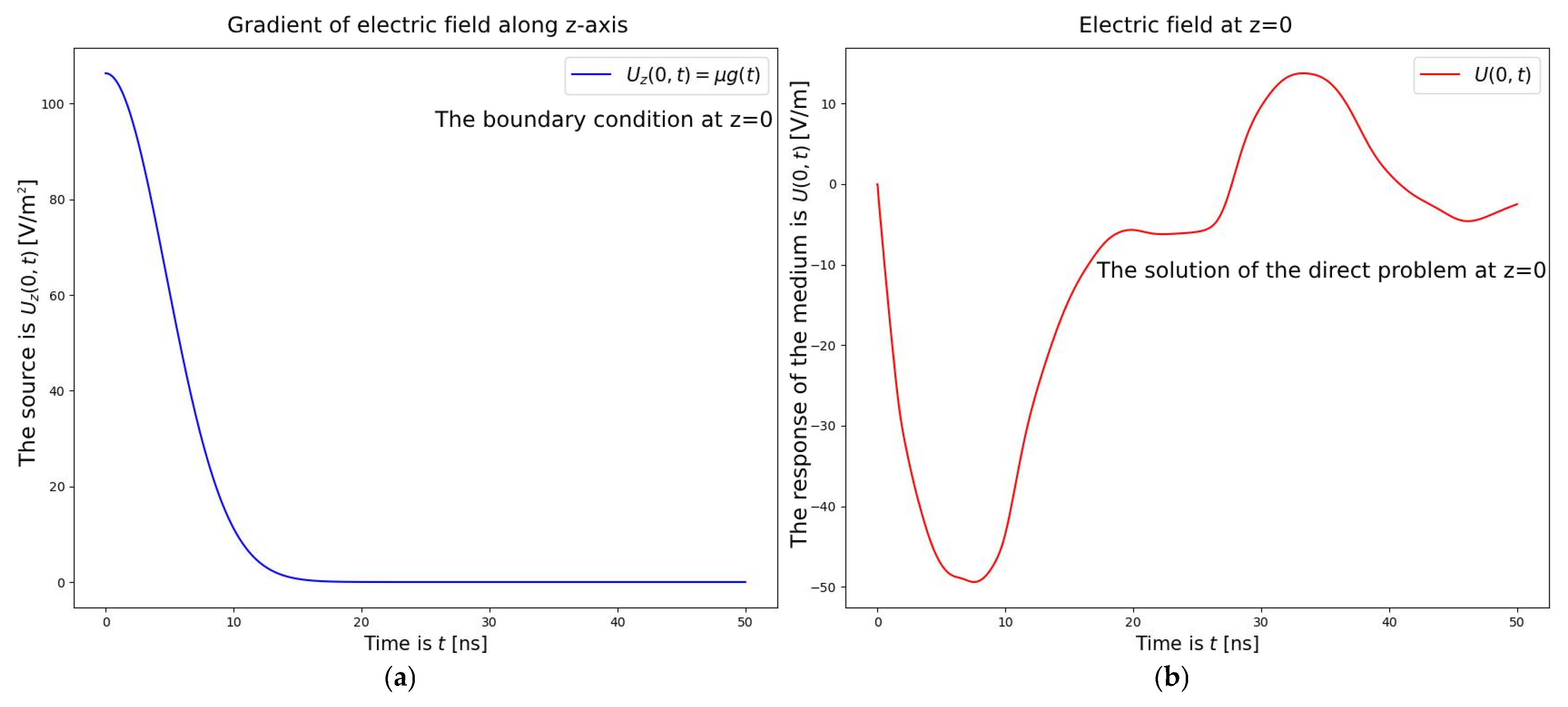
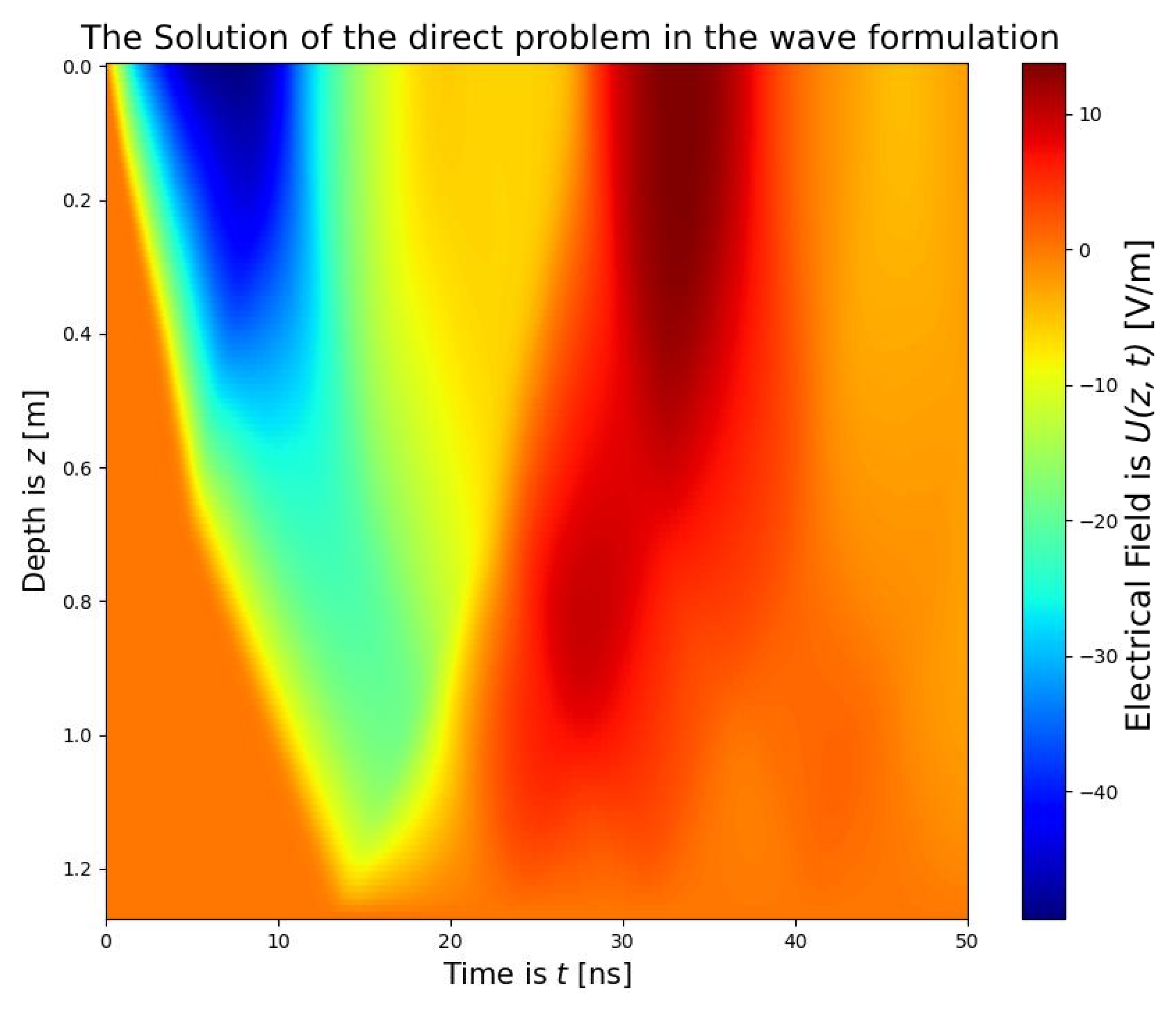
The graphs of the source (8), the medium’s response (5), and the solution of the problem (6)–(8) in the wave formulation are presented below.

The Gaussian function (9) with the parameter $\alpha ={1.5\times 10}^8$ was selected to represent the source (Figure 9).

In Figure 9 and Figure 10, time $t$ ranges from 0 to 50 ns, and depth $z$ ranges from 0 to 1.27 m. Both the solution and the medium’s response correspond to the electrical voltage, while the source corresponds to the gradient of the electrical voltage along the $Oz$-axis. Electrical voltage is measured in [V/m], and its gradient is measured in [V/m²].

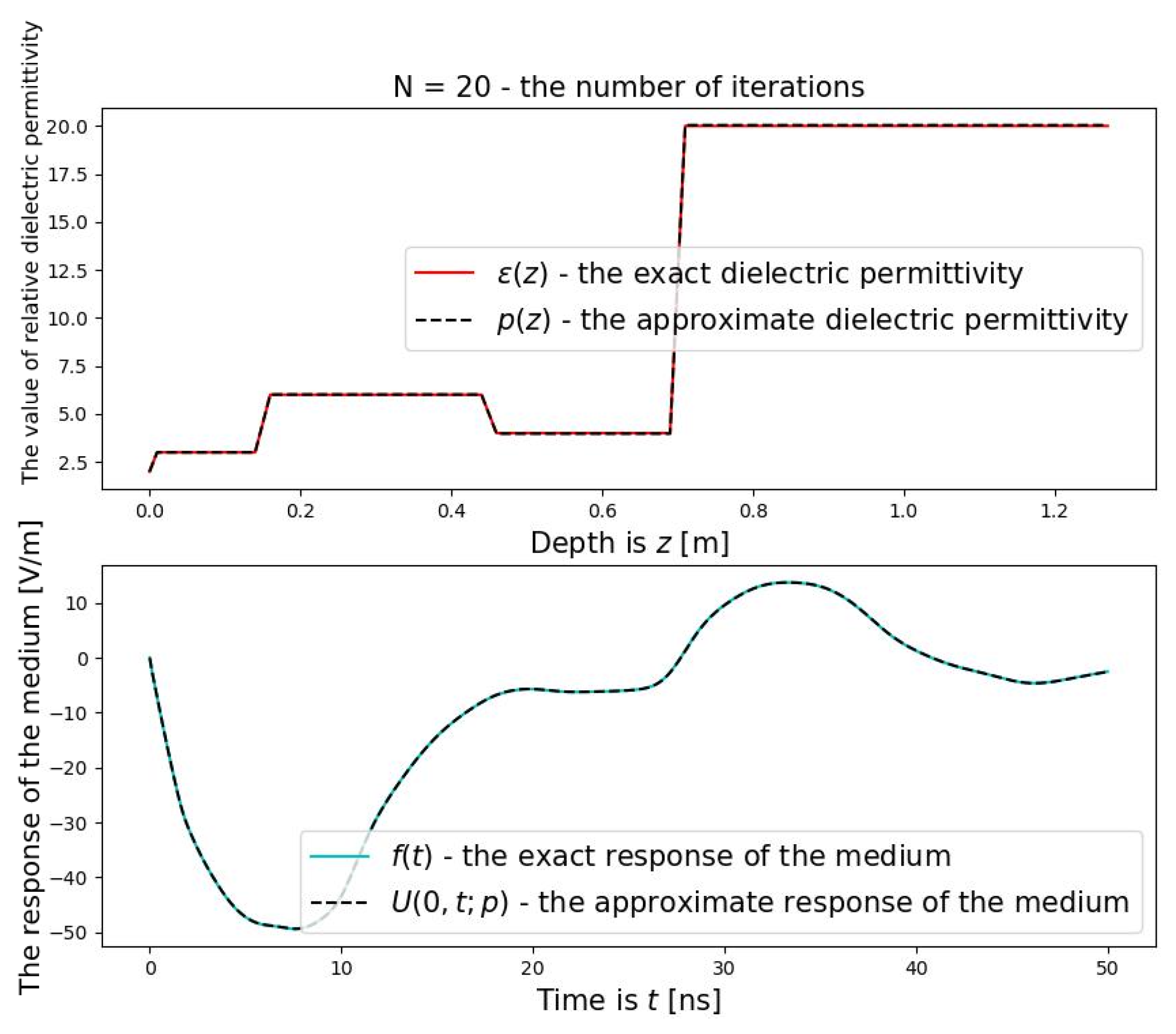
In the case of the wave formulation, all layers of the underground medium were successfully reconstructed. The reconstruction was achieved in 28 iterations with a termination parameter $\delta ={10}^{-4}$ for the optimization method (19), resulting in an accuracy of 10−2 (relative error less than 1%), which represents an excellent outcome. The convergence of the optimization method is highly sensitive to the choice of the initial approximation. The initial approximations of the relative dielectric permittivity were set to 1, representing the minimal physically meaningful value. The initial approximation was selected to be constant across the entire domain and as low as possible (see Figure 11, indicated by the dashed line). The exact values (experimental data obtained from the CartScan software [31]) and the approximate values of the dielectric permittivity are presented in

Table 2. Exact and approximate values of relative dielectric permittivity.

Layer Number	1-st Layer	2-nd Layer	3-rd Layer	Subgrade Layer
${\epsilon }_r$	3.0	6.0	4.0	20.0
$p$	2.99639	5.99996	3.99539	20.00647

${\epsilon }_r$ and $p$ represent the exact and approximate relative dielectric permittivities, respectively.

.

The norm of the difference between the exact and approximate solutions is

$${‖\epsilon \left(z\right)-p\left(z\right)‖}_{L_2}=5.52\times {10}^{-3}.$$

(32)

Figure 11, Figure 12, Figure 13 and Figure 14 present graphs of the approximations and exact values of the dielectric permittivity, as well as the medium response in the wave formulation, for varying numbers of iterations. Note that Figure 11, Figure 12, Figure 13 and Figure 14 illustrate the relative dielectric permittivity, which are dimensionless quantities.

4. Discussion

The results obtained demonstrate the high accuracy of reconstructing the dielectric permittivity of pavement layers, as evidenced by the low level of discrepancy between the exact and reconstructed values. In particular, the average relative error of ${\epsilon }_r$ reconstruction was less than 1%, and the algorithm converged in 28 iterations, as shown in the upper part of Figure 14. These results demonstrate the stability of the proposed discrete method for interpreting radar images.

The developed algorithm is based on solving the adjoint problem and minimizing the quadratic functional of the discrepancy between the measured and modeled environmental responses. An important advantage of the method is the preservation of physical laws, particularly the law of conservation of energy, through the use of conservative finite-difference schemes. This ensures physical consistency and numerical stability when modeling the propagation of electromagnetic waves in a vertically inhomogeneous medium.

Based on this review, the following methods can be identified for solving the interpretation problem (determining the geoelectric section):

• engineering and technical methods [25];
• selection methods and regularization methods [20];
• machine learning methods [12,29,30];
• optimization methods [19,21].

In comparison with the aforementioned methods, the optimization method demonstrates superior practicality for solving the problem. As noted earlier, it is theoretically justified [22], analyzed for convergence of the iterative steepest descent method [33], and its convergence, along with conservation and uniformity properties, is numerically validated using experimental data (see the upper part of Figure 14).

A comparison with existing approaches, presented in

Table 3. Comparative analysis of existing methods for radar image interpretation.

Criteria	Engineering Methods [25]	Regularization Methods [20]	Machine Learning [12,29,30]	Proposed Method [19,21]
Physical validity	Low	Moderate	Low	High
Average reconstruction error (${\epsilon }_r$)	$~15-20\%$	$~10-15\%$	$~5-10\%$	$<1\%$
Computation time per profile (seconds)	$<1$	$~3-5$	$~1800-3600$	$~60-120$
Data volume	Minimal	Moderate	High	Moderate
Customization flexibility	Limited	Implementation-dependent	Model-dependent	Flexible (thickness, ${\epsilon }_r$, steps)
Need for a priori data	No	Desirable	Yes	Yes (initial approximations based on physical validity)
Environmental geometry	Simplified	Linear	Arbitrary	Piecewise constant

, shows that, in contrast to traditional engineering methods based on heuristic approximations and regularization schemes (e.g., SVD or Tikhonov’s method), the proposed method achieves higher accuracy. Compared to machine learning methods, the developed approach eliminates the need for labeled training datasets, making it more practical in real-world data acquisition scenarios.

The formulation of the problem for the geoelectric equation considered here is physically justified in [20,22]. The rationale behind these explanations is as follows. Assuming that the source is a long cable located on the ground surface and that the dielectric permittivity depends solely on depth (which is valid in this case, as the road surface consists of layers), the system of Maxwell’s equations can be simplified. Specifically, the equations depend only on the horizontal component of the electric field, while the magnetic field components depend on two variables.

As described in [22], the equations can be further simplified, and by performing the Fourier transform on one spatial variable, one obtains a one-dimensional formulation of the geoelectric equation. Since the inverse coefficient problem under consideration is ill-posed, the theoretical issues of uniqueness and stability are addressed in [22]. Further details regarding the aforementioned calculations can be found in this work.

To solve the inverse coefficient problem, the optimization method was employed. The convergence of the steepest descent method for solving the inverse coefficient problem was first proven in [33].

Future research directions include extending the approach to two-dimensional and three-dimensional heterogeneous media, as well as integrating machine learning methods and neural networks. This will enable the automatic classification of layers, adaptive adjustment of model parameters, and anomaly recognition based on extensive radar datasets.

5. Conclusions

In this study, a discrete numerical algorithm was developed and implemented to solve the practical problem of reconstructing a geophysical section aimed at determining the physical characteristics of the pavement, such as the dielectric permittivity of the layers. The relevance of this work stems from the necessity to develop highly accurate and reproducible methods for monitoring road infrastructure conditions.

A non-destructive subsurface radar sounding method employing an OKO-2 series GPR was utilized in this research. Primary signal processing was performed in the CartScan software environment, where noise removal, trace alignment, and AGC were applied. The obtained radar images served as the basis for subsequent numerical modeling based on Maxwell′s equations.

To determine the geoelectric properties of the medium, algorithms for numerical solutions of direct and adjoint problems with conservative properties were developed. This enabled the implementation of an optimization approach to solving the inverse problem based on minimizing the quadratic functional between the theoretical and measured responses of the medium.

The proposed algorithm outperforms traditional engineering methods in terms of accuracy, interpretability, and noise tolerance. In contrast to machine learning approaches, it does not require large training datasets and preserves the physical meaning of the parameters. This method is non-destructive and obviates the need for core drilling, thereby significantly reducing costs in terms of both time and resources during the inspection of road infrastructure.

Through experimental studies conducted with the CartScan software, which enables the determination of layer-specific dielectric permittivity, this data was utilized to test the proposed algorithm. Based on numerical calculations, as shown in the upper part of Figure 11, the lowest value of the dielectric permittivity (${\epsilon }_r=1$) was chosen as the initial approximation. A discrete algorithm was developed for solving the optimization problem of reconstructing the dielectric permittivity. The algorithm achieved an accuracy of ${10}^{-2}$ within 28 iterations, as shown in the upper part of Figure 14 and defined by the error formula (32).

Starting from the initial approximation, assumed to be a constant ${\epsilon }_r=1$ at all points, the algorithm successfully reconstructed a vertically inhomogeneous four-layer medium. This demonstrates that the developed algorithm can be effectively applied in practice at any point along the route to assess the condition of the road surface.

Future work may focus on extending the method to two-dimensional and three-dimensional models, as well as integrating it with neural network approaches to automate the interpretation of GPR data.