Mitigating Multicollinearity in Induction Motors Fault Diagnosis Through Hierarchical Clustering-Based Feature Selection

Abstract

This paper addresses the challenge of multicollinearity among input features in induction motor (IM) fault diagnosis, which often degrades the performance and reliability of machine learning classifiers. A novel feature selection approach based on agglomerative hierarchical clustering (AHC) is proposed to mitigate feature redundancy and enhance model generalization. The method is applied using only voltage and current signals, excluding vibration or temperature data, to improve noise immunity and facilitate practical deployment. Experimental validation demonstrates the effectiveness of the AHC framework across multiple classifiers, particularly Support Vector Classifiers (SVCs) and Artificial Neural Networks (ANNs). Compared to random forest-based feature selection, AHC yields a 2% increase in accuracy for SVCs and a 0.6% improvement for ANNs. Moreover, both classifiers exhibit enhanced balance across fault categories, with macro-average recall and F1-score improvements of approximately 1.5%. These findings highlight the ability of AHC to handle complex fault scenarios, which offer a more efficient and generalized fault diagnosis model compared to ensemble methods-based feature selection.

1. Introduction

Considering its transferability to industry, the impact of feature selection on the effectiveness of fault diagnosis techniques for induction machines (IMs) is frequently overlooked. Although some recent studies have incorporated optimal feature selection into their methodologies, they often fail to offer solutions that are intelligently tailored to industrial applications [1,2]. Many recently developed methodologies focus heavily on utilizing highly sophisticated optimization algorithms to identify optimal feature sets; however, the results of these algorithms are often inherently biased by the formulation of the objective functions on which they heavily depend [3,4,5,6]. On the other hand, the availability of multiple data sources and the relatively modest computational power of most personal computers, compared to industrial settings, often motivate researchers to capture as many features as possible to test their Artificial Intelligence (AI)-based developed algorithms. While this approach aims to enhance model performance, it frequently leads to redundancy and noise, underscoring the crucial role of feature selection. Typically, IM fault detection and diagnosis techniques can be categorized based on the features employed in vibration analysis, stator current measurements, temperature monitoring, thermal imaging, acoustic emissions, spectral analysis, or a combination of these methods [7]. Among these features, vibration analysis and stator current measurements are the most appealing for industrial applications. Therefore, the following is a summary of the latest fault diagnosis methodologies based on these fundamental measurements.

1.1. Vibration-Based Fault Diagnosis

In [8], an online fault diagnosis system was developed using random forest (RF) and Extreme Gradient Boosting (XGBoost) algorithms, demonstrating a 15% performance improvement for XGBoost with optimized hyperparameters and a 1107% rise in training time. The issue of feature selection was discussed in [1,2,4,9]. In [1], an IM fault diagnosis framework based on the Light Gradient Boosting Machine (LightGBM) was developed. The study employed vibration signals and Recursive Feature Elimination (RFE), in addition to Bayesian hyperparameter optimization, which resulted in an accuracy of 100% across varying operating conditions. In [4], fault identification using acoustic entropy feature selection and the Hierarchical Adaptive Neuro-Fuzzy Inference System (HANFIS) was proposed. The study in [9] used deep features extracted from vibration spectrograms, combined with Ensemble Deep Models Features Extraction (EDMFE) and optimized via ensemble feature selection (EFS), achieving 100% accuracy in less than 70 s. Similarly, adaptive feature selection for rolling bearing fault diagnosis was addressed in [2]. A total of 240 features were extracted. Then, a three-layer feature selection algorithm was applied to filter and optimize the feature set. The suggested three-layer algorithm comprised the Chi-square test, Variance–Relief-F, and hierarchical clustering algorithms. Lastly, optimized features were then classified using Fuzzy C-Means (FCM) clustering, resulting in a more complex and demanding fault diagnosis process compared to traditional methods.

Moreover, in [10], a hybrid multi-model feature fusion approach was investigated for detecting multiple faults, including rotor and bearing defects. Similarly, in [11], the study employed fourteen dimensionality reduction methods, significantly reducing computational time by only 21%. The results of applying mutual information and Analysis of Variance (ANOVA) F-tests for feature selection and Logistic Regression (LR) and SVC for fault detection were reported in [12]. The study emphasized the superiority of the optimized hyperparameters SVC model compared to LR.

Similarly, a combination of the Hilbert spectral envelope with RF for detecting and locating bearing defects was presented in [13]. The proposed combination achieved an accuracy of 99.94%. In [14], a Convolutional Long Short-Term Memory (CLSTM) architecture for fault detection and diagnosis (FDD) of rotating machinery was introduced. The proposed model achieved 100% accuracy with short input data, making it suitable for real-time monitoring. Studies [15,16] addressed fault diagnosis for Variable Frequency Drive (VFD)-fed IMs. In [15], tri-axial vibration signals were used for fault diagnosis across varying operating frequencies, with discrete wavelet transform (DWT)-based feature extraction improving diagnostic accuracy by 12%. Meanwhile, the integration of Internet of Things (IoT) technology for online fault diagnosis of IMs was explored in [16].

1.2. Current Signature-Based Fault Diagnosis

While vibration analysis is a well-established technique for detecting faults, specifically mechanical faults, it presents several limitations for industrial applications [4]. Vibration sensors are often expensive, require precise installation, and are susceptible to environmental noise, which adversely affects the performance of fault diagnosis techniques [17]. Additionally, accessing motor bearings or the motor itself for sensor placement or even external attachments can be challenging in certain operational environments. In contrast, current signature analysis (CSA), which can be easily captured at any point along the cables, offers a more cost-effective and non-intrusive solution for the fault diagnosis of IMs. The application of CSA for IM fault diagnosis has been extensively studied, with various techniques developed to enhance fault detection, classification, and location [18].

In [5], a model based on empirical mode decomposition (EMD), multi-resolution analysis (MRA), and fast Fourier transform (FFT) was proposed to extract 144 features from current signals. A feature selection process combining symmetrical uncertainty (SU), binary grey wolf optimization (BGWO), and emperor penguin optimizer (EPO) was employed and achieved an accuracy of 99.54% on the Case Western Reserve University (CWRU) benchmark and 99.52% on the machinery failure prevention technology (MFPT) dataset. Similarly, the Hilbert–Huang transform (HHT) was applied to extract features in [19], and the extracted features were ranked using a feature selection based on distance discriminant (FSDD). Combined with a backpropagation neural network (BPNN) algorithm, the proposed technique reported an accuracy of 98.98%. However, the high false-negative rate (13.66%) suggests that further refinement is needed for more precise fault detection.

The synergetic combination of particle swarm optimization (PSO) and BPNN was presented in [20]. The proposed approach initially extracted 50 features and reduced them to nine via a mean impact value (MIV) algorithm. The model maintained an accuracy of 99.4% while reducing computational time by 9%. However, the use of 50 hidden layers increased the risk of overfitting. In [21], a hybrid genetic binary chicken swarm optimization (HGBCSO) algorithm was adopted for feature selection. The model used local mean decomposition (LMD) and wavelet packet decomposition (WPD) to reduce data dimensions and extract essential features. On the other hand, a practical edge-computing approach for motor fault diagnosis using CSA was also presented in [22]. This method utilized the affordable Arduino platform for data acquisition, signal processing, and model deployment, with a focus on real-world implementation. The model produced positive results when tested on electrical machines.

A different approach was introduced in [23], which utilized singular analysis to detect faults in stator current signals. The method decomposed the current time series into singular triples using Hankelization matrices. However, the complexity and computational demands of the singular analysis and matrix Hankelization processes limit its practicality for real-world industrial applications. Additionally, recent research that emphasizes the role of AI and deep learning techniques in fault diagnosis is reviewed in [24,25], and [7,26,27], respectively.

Alternatively, feature reduction techniques offer an attractive solution to eliminate the curse of dimensionality. Thus, [28] proposed a fault classification technique using radial basis function neural networks (RBFNNs) and probabilistic neural networks (PNNs), incorporating principal component analysis (PCA) for feature reduction. Similarly, [29] employed receiver operating characteristic (ROC) curves and t-distribution stochastic neighbor embedding (t-SNE) for dimensionality reduction, improving classification accuracy by 2–3% and reducing data dimensions by 70%.

In a few words, regardless of the source from which the features are extracted, the difficulty in identifying the most influential features remains the major issue. If not adequately addressed, high feature correlation and redundancy can lead to overlapping or redundant information, exacerbating the risk of multicollinearity, a condition where highly correlated features compromise the performance of the IM diagnostic model. While several studies have explored feature selection techniques, they often fail to reduce intercorrelations among features chosen explicitly. In fact, many existing methodologies deliberately retain correlated features to maximize accuracy in training performance, yet this approach risks hindering model generalization and limiting applicability in real-world industrial environments.

To overcome this issue, this study proposes a nonintrusive, industry-oriented fault diagnosis strategy that leverages agglomerative hierarchical clustering (AHC) in conjunction with the Spearman rank-order correlation coefficient for feature selection. While hierarchical clustering and clustering-based feature selection have been explored across various domains, including biomedical signal processing (e.g., references [30,31,32,33]) and vibration-based fault diagnosis (references [4,9]), these existing methods do not fully address the specific challenge of multicollinearity in harmonic-based fault features within induction motor (IM) diagnostics. By systematically quantifying feature dependencies and eliminating redundancy, the proposed method directly addresses the challenges posed by multicollinearity. Moreover, while numerous fault types exist, both mechanical and electrical, a technical report issued by the Electric Power Research Institute (EPRI) indicates that approximately 70% of IM failures result from either bearing defects (~40%) or stator faults (~30%), including single-phase loss [8,26]. Therefore, this study focuses on detecting mechanical faults using electrical signal analysis as a nonintrusive alternative to conventional vibration and thermal approaches.

Additionally, experimental validation using the NI CRIO-9056 platform confirms the effectiveness of the developed technique, while comparative analysis against established techniques, including random forest-based feature selection, demonstrates its advantages in improving classification robustness and minimizing overfitting risks.

Novel Contributions in the Context of Existing Approaches:

• Unlike many prior studies that rely on vibration or acoustic signals (as in [1,2,4,9]), the proposed work in this study leverages voltage and current phasor measurements to diagnose faults in IMs. This nonintrusive method eliminates the need for expensive or difficult-to-install sensors while ensuring minimal disruption to ongoing industrial processes.
• Most conventional fault diagnosis methods rely on statistical [28,30,34] or deep feature extraction techniques [7,9,27] applied to vibration or acoustic data for bearing fault detection. In contrast, the proposed approach leverages harmonic-based features extracted from voltage and current phasors. This methodology captures subtle variations that indicate bearing-related faults.
• While hierarchical or clustering-based methods have been used in other domains (e.g., [31,32] use k-means clustering for feature selection, and [33] applies hierarchical clustering in cancer diagnosis), this work is distinct because it directly targets the multicollinearity challenge in IM fault diagnosis, a crucial factor that many existing methods do not explicitly address.
• The practical viability of the developed method is demonstrated via validation on the NI CRIO-9056 platform, confirming its applicability in real-world scenarios. Furthermore, this study provides a rigorous comparative analysis against established feature selection techniques (such as random forest feature selection) and evaluates performance using three high-performance estimators (RFC, ANN, and SVC). This comprehensive evaluation underscores that the AHC-based approach not only improves classification performance but also mitigates the overfitting risk associated with multicollinearity, which is a gap in the current literature.

To the best of our knowledge, this study represents the first application of an AHC-based feature selection strategy tailored for fault diagnosis in electrical machines. By explicitly leveraging harmonic-based features and addressing multicollinearity through Spearman correlation and hierarchical clustering, this approach offers a distinct advantage over previous clustering-based feature selection methods. In doing so, it bridges a critical gap in fault diagnosis methodologies, ensuring both high accuracy and strong generalization for industrial applications.

The structure of this work is organized into seven sections, followed by references. The introduction establishes the objectives and significance of this study. Next, Feature Engineering outlines the process of extracting voltage and current phasor-based features, followed by an in-depth discussion on feature selection using the AHC algorithm. Section four examines the machine learning algorithms employed, while section five details the research methodology. The findings and their implications are presented in section six, leading to the final section, which synthesizes key conclusions and proposes directions for future research.

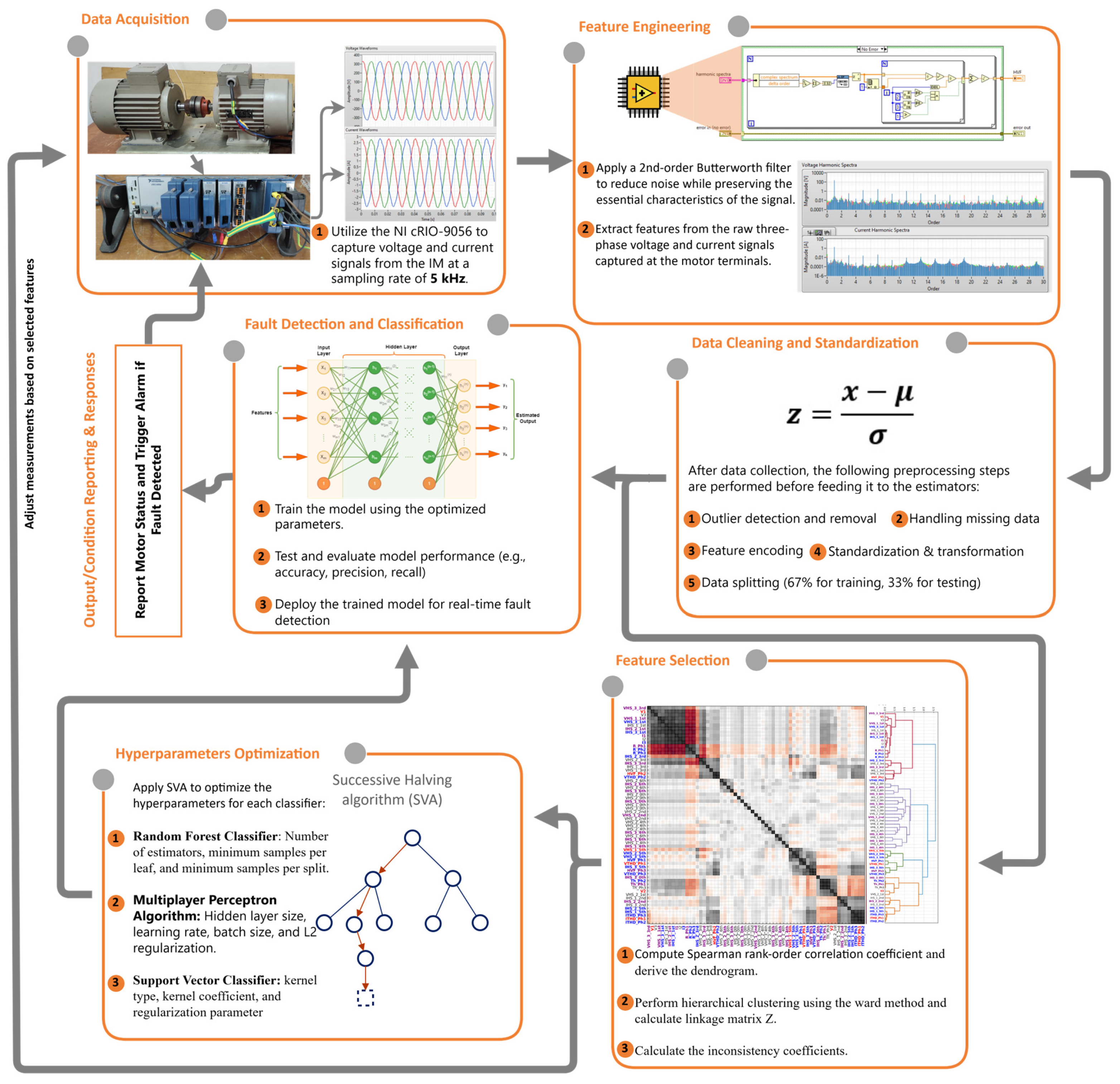
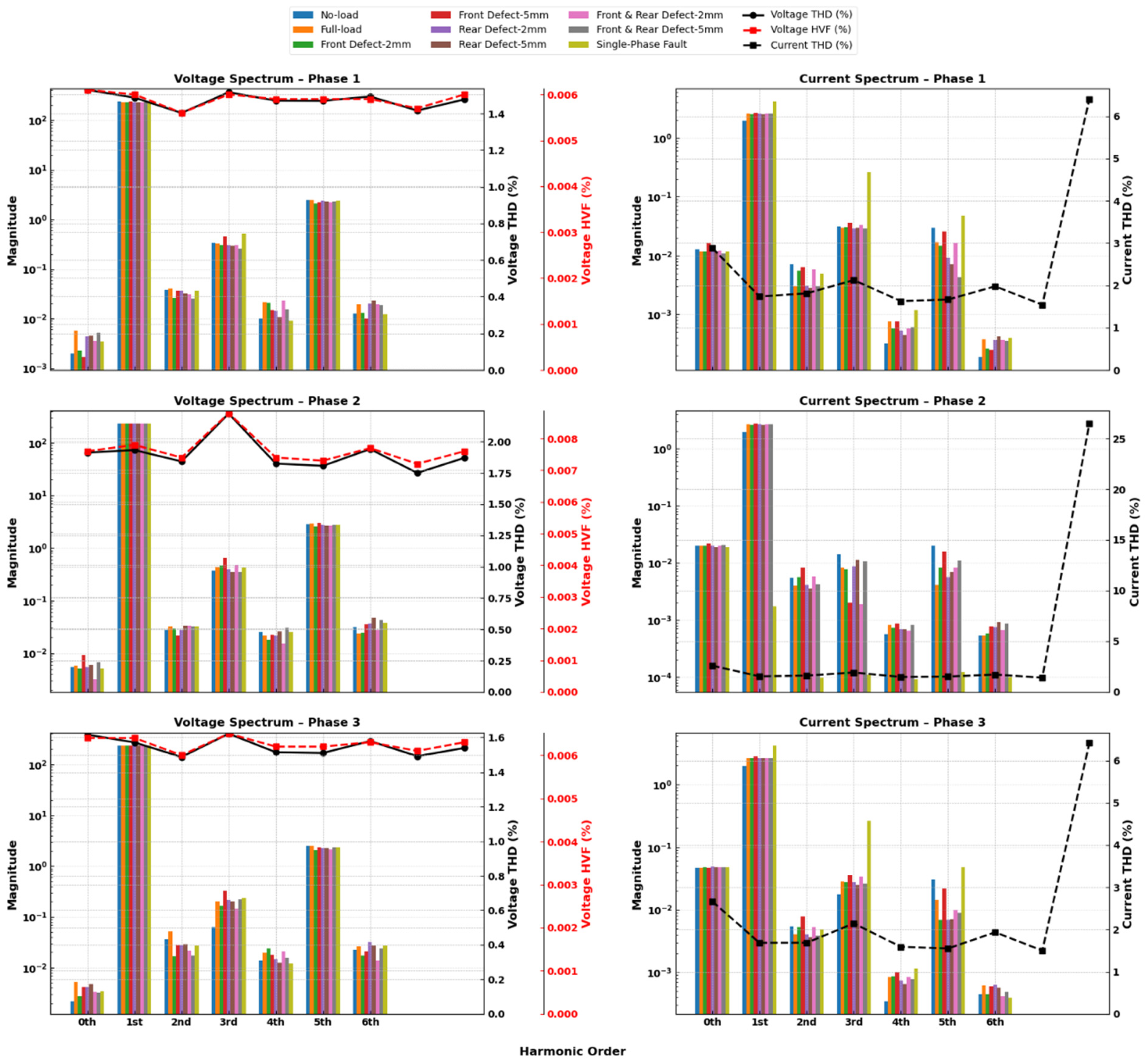
2. Feature Engineering

Considering the importance of feature extraction for effective fault diagnosis, this investigation adopts a unique approach, relying exclusively on voltage and current phasors captured directly from the terminals of the machine under test. Even though feature extraction provides valuable insights into machine status, it results in data sets that are susceptible to multicollinearity. Given the uncertainty surrounding the optimal feature set, however, this stage aims to collect as many features as possible and subsequently employ the developed algorithm to identify the optimal subset. Therefore, in addition to three-phase winding impedance calculations, a set of features is derived and covered in the following subsections. The selected features, namely the fast Fourier transform (FFT) spectrum of voltage and current signals, total harmonic distortion (THD), and the harmonic voltage factor (HVF), were chosen based on their strong theoretical foundation and proven effectiveness in power quality assessment and electrical fault diagnostics. Specifically, the FFT enables transformation of time-domain phasor data into frequency-domain representations, thereby revealing harmonic components and frequency signatures associated with specific fault types [14]. Similarly, THD, as defined by IEEE Std. 519-2022 [35], quantifies the cumulative distortion effect of higher-order harmonics on the fundamental waveform. THD is particularly sensitive to nonlinear loading and imbalance scenarios, making it a robust indicator of both electrical and mechanical anomalies [22].

Additionally, the HVF provides a normalized index for evaluating the relative contribution of individual harmonic orders to the overall signal. By evaluating the ratio of specific harmonic magnitudes to the fundamental waveform, HVF enables the detection of harmonic-rich conditions that are often overlooked by traditional metrics, according to IEC 60034-1 [36,37].

Together, these features create a multidimensional input space, capturing both linear and nonlinear fault behaviors. This ensures that the feature selection algorithm can effectively isolate the most discriminative attributes, ultimately improving fault classification accuracy and system reliability.

2.1. FFT Analysis of Voltage and Current Signals

A comprehensive FFT analysis of voltage and current signals was performed to accurately extract the harmonic spectrum. However, FFT remains a simple yet effective method for calculating the Fourier transform, as expressed in (1) [34].

$$X\left[n\right]=F\left\{x\left(t\right)\right\}={\int }_{-\infty }^{+\infty }x\left(t\right) e^{-j2\pi ft}dt$$

(1)

where $x\left(t\right)$ denotes the captured signals, representing either voltage or current, in the time domain, and X[n] signifies the transformed signal in the frequency domain. Given that the signal is a discrete sequence of samples, Equation (1) can be expressed in alternative forms, as illustrated in (2) or (3).

$$X\left[k\right]=\sum _{n=0}^{N-1}{x}_n e^{-j2\pi \left({\displaystyle \frac{kn}{N}}\right)}$$

(2)

$$X\left[k\right]=\sum _{n=0}^{N-1}{x}_n\left[cos \left(2\pi \left({\displaystyle \frac{kn}{N}}\right)\right)-j sin\left(2\pi \left({\displaystyle \frac{kn}{N}}\right)\right)\right] , k=\mathrm{0,1},2\dots , (n-1)$$

(3)

where ‘x’ symbolizes the sequence of voltage or current samples, while ‘n’ represents the count of samples in the dataset.

This study conducted an extensive harmonic analysis, extending the calculations to the 30th order for each phase, encompassing both voltage and current quantities. However, the features utilized for classifier training were intentionally limited to the first seven harmonic orders per phase, ensuring a focused and manageable dataset. This selection resulted in 42 unique features representing the entire three-phase circuit, optimizing classification performance while maintaining computational efficiency.

2.2. Total Harmonic Distortion

Similarly, the THD was calculated as outlined in (4). Incorporating THD, which quantifies the harmonic content in both voltage and current signals, into the feature set, significantly enhanced the predictive power of the estimators, enabling a more precise assessment of the actual condition of the IM.

$$\mathrm{T}\mathrm{H}\mathrm{D}\left[\mathrm{\%}\right]=\sqrt{{\displaystyle \frac{{\sum }_{i=2}^{i_{max}}{X}_i}{X_1}}}$$

(4)

where X_i symbolizes the magnitude of harmonic components, which can be either voltage or current samples. X₁ refers to the fundamental component, and i_max signifies the highest designated order. Notably, the total number of features calculated using the THD measurement for the three-phase system is six features.

2.3. Harmonic Voltage Factor

Likewise, the investigation included the computation of the harmonic voltage factor (HVF), a critical index widely used to evaluate electrical system quality. The mathematical expression for HVF is outlined in (5). As is apparent from (5), the HVF serves as a rigorous indicator for distinguishing the presence of harmonic distortions. Hence, it can be considered as an additional indicator that is highly responsive to anomalies associated with a faulty machine.

$$\mathrm{H}\mathrm{V}\mathrm{F}=\sqrt{{\displaystyle \frac{V_5^2}{5}}+{\displaystyle \frac{V_7^2}{7}}+{\displaystyle \frac{V_{11}^2}{11}}+\dots +{\displaystyle \frac{V_n^2}{n}}}$$

(5)

In this context, HVF represents the harmonic voltage factor, with $V_n$ denoting the magnitude of harmonic voltage, and ‘$n$’ signifying the order of the voltage signals’ odd harmonics. This features expansion contributes to a better understanding of the electrical fault’s behavior and potential deviations from the norm, enabling a more profound comprehension of the system’s complexities. By including an additional three features for the three-phase voltages, the total number of features in this study is increased to sixty-three features.

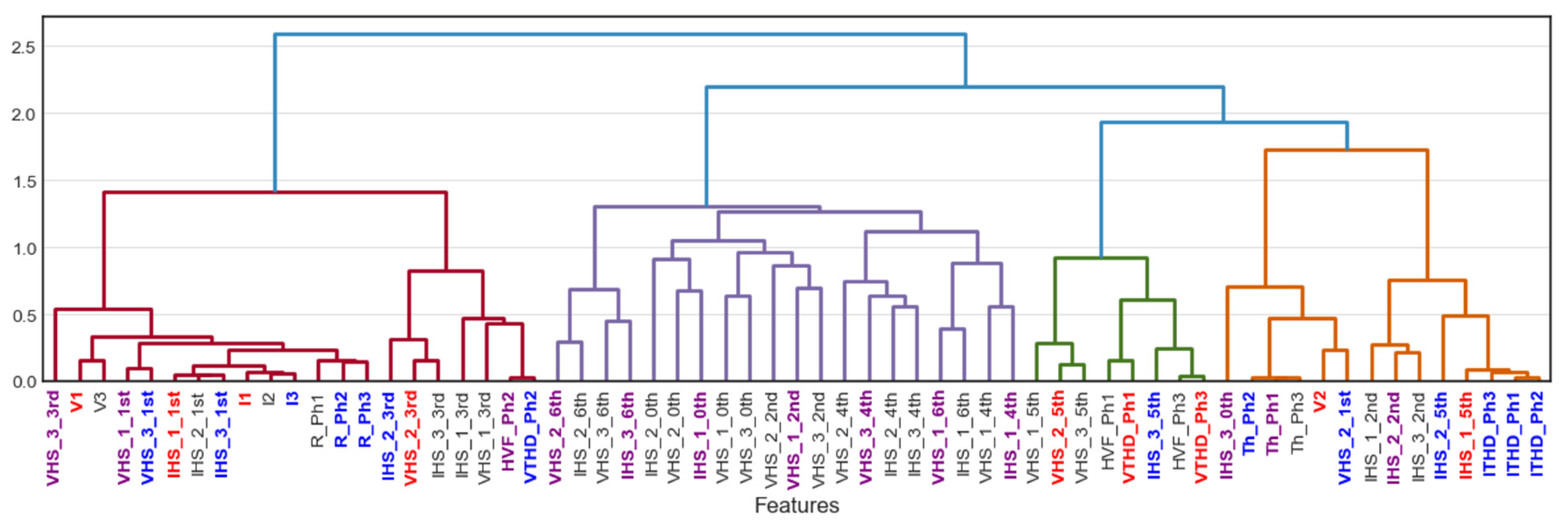
3. Feature Selection Using Agglomerative Hierarchical Clustering

When the feature space exhibits collinearity, permuting one feature often has minimal impact on the overall performance of the estimator because the estimator can still extract similar information from other correlated features. This overlap can adversely affect the estimator’s effectiveness. In other words, by selecting one representative feature from each cluster, the characteristics of the entire cluster are effectively captured and included in the assessment process of the machine’s status, thus ensuring an efficient analysis while minimizing redundancy [30,31,32,33].

The Spearman rank-order correlation coefficient, denoted by $r_s$, is a Pearson correlation coefficient, denoted by $\rho$, and is calculated using the ranked variables of the dataset. It quantifies the degree of connection between variables, features in this case, while considering their ranked values rather than raw data, providing a robust measure of monotonic relationships within the dataset ($U$). For the m-th feature $U=[F_1, F_2, F_3,\dots ,F_m]$, the $r_s$ for two features of N observations is computed as follows [35,36]:

$$r_{s\left(i,j\right)}={\displaystyle \frac{12{\sum }_{n=1}^N\left\{\left[R\left(F_{i,n}\right)-\left(\frac{N+1}{2}\right)\right]\left[R\left(F_{j,n}\right)-\left(\frac{N+1}{2}\right)\right]\right\}}{N\left(N^2-1\right)}}$$

(6)

Or

$$r_{s\left(i,j\right)}=1-{\displaystyle \frac{6{\sum }_{n=1}^N\left\{d_{\left(ij\right),n}^2\right\}}{N\left(N^2-1\right)}}$$

(7)

where $d_{ij}=R\left(F_i\right)-R\left(F_j\right), i,j=1, 2, 3, \dots , m$, and $R\left(F_i\right)$ and $R\left(F_j\right)$ signify the rank of samples in features $F_i$ and $F_j$. The Spearman correlation matrix for dataset Z can be formulated as follows:

$$\left[\begin{array}{cccc}1& 1-{\displaystyle \frac{6{\sum }_{n=1}^N\left\{R\left(F_1\right)-R\left(F_2\right)\right\}}{N\left(N^2-1\right)}}& \dots & 1-{\displaystyle \frac{6{\sum }_{n=1}^N\left\{R\left(F_1\right)-R\left(F_m\right)\right\}}{N\left(N^2-1\right)}}\\ 1-{\displaystyle \frac{6{\sum }_{n=1}^N\left\{R\left(F_2\right)-R\left(F_1\right)\right\}}{N\left(N^2-1\right)}}& 1& \dots & 1-{\displaystyle \frac{6{\sum }_{n=1}^N\left\{R\left(F_2\right)-R\left(F_m\right)\right\}}{N\left(N^2-1\right)}}\\ ⋮& ⋮& \ddots & ⋮\\ 1-{\displaystyle \frac{6{\sum }_{n=1}^N\left\{R\left(F_m\right)-R\left(F_1\right)\right\}}{N\left(N^2-1\right)}}& 1-{\displaystyle \frac{6{\sum }_{n=1}^N\left\{R\left(F_m\right)-R\left(F_2\right)\right\}}{N\left(N^2-1\right)}}& \dots & 1\end{array}\right]$$

(8)

Once the Spearman correlation coefficient matrix is obtained, the subsequent step involves applying the AHC algorithm, which is used to compute the distance linkage matrix. However, to obtain the linkage matrix in AHC, the choice of distance or dissimilarity measure in conjunction with the linkage criterion is essential for determining the similarity between data points or clusters. The most commonly used linkage methods include single linkage, complete linkage, Ward’s method, and the average linkage method, each offering distinct insights into the structure of the data and influencing how clusters are defined [32]. As a matter of fact, linkage methods are specifically formulated to calculate the distance, indicated as $D_{ij}$, between two clusters, i and j. The general representation of this distance equation can be formulated as follows:

$$D_{ij}=g\left(F_i,F_j\right)$$

(9)

In (9), $D_{ij}$ represents the distance or dissimilarity between data points or clusters i and j, where $F_i$, and $F_j$ are the feature vectors, and $g$ is a distance or dissimilarity function that quantifies the dissimilarity between the data points, clusters or feature vectors in this study. However, considering the scope of this work, the Ward linkage method, utilizing the Euclidean distance, was employed to update the linkage matrix. For two data points x and y in the n-dimensional space, the Euclidean distance can be formulated as follows:

$$d_E(x,y)=\sqrt{{\sum }_{i=1}^n{\left(x_i-y_i\right)}^2}$$

(10)

Consider a scenario in which a cluster $K$ emerges through the combination of original observations, namely $K\left[0\right], K\left[1\right], ..., K[n_K-1]$, as a result of the fusion of clusters $i$ and $j$. Within this framework, another cluster is introduced, labeled as $L$, which is part of the forest but distinct from cluster $K$. Cluster $L$ contains $n_L$ original objects, denoted as $L\left[0\right], L\left[1\right], ..., L[n_L-1]$. By utilizing the Ward variance minimization algorithm, the computation of the new entry $D_{ward}(K,L)$ can be executed as follows [37]:

$$D_{Ward}\left(K,L\right)={\displaystyle \frac{n_K{n}_L}{n_K+n_L}}{d}_E(K,L)$$

(11)

In (11), $D_{Ward}$ represents the distance between clusters $K$ and $L$ under consideration for merging, where $n_K$ and $n_L$ correspond to the number of data points within clusters $K$ and $L$, respectively. $d_E$ is the distance between the centroids of clusters $K$ and $L$ using the Euclidean distance metric. However, most modern algorithms often employ a more computationally efficient formulation to derive the inter-cluster distance, which is expressed mathematically as follows [38]:

$$D_{Ward}\left(K,L\right)=\sqrt{{\displaystyle \frac{{(n}_L+n_I\left)d_E\right(L,I)}{S}}+{\displaystyle \frac{{(n}_L+n_J\left)d_E\right(L,J)}{S}}-{\displaystyle \frac{{(n}_L\left)d_E\right(I,J)}{S}}}$$

(12)

where ${S=n}_L+n_I+n_J$. ${ n}_L, n_I$, and $n_J$ are the numbers of data points in clusters $L$, $I$, and $J$, respectively.

Once the AHC is performed and the linkage matrix is obtained, the transition to flat clusters can be achieved. This transition from hierarchical to flat clusters necessitates the application of inconsistency criteria. The inconsistency criteria allow the selection of specific levels of detail by identifying where to cut branches in the dendrogram. The inconsistency coefficient at a specific merge level $i$ in the hierarchical clustering tree can be formulated as follows [39]:

$$\mathrm{inconsistency} \mathrm{coef}.={\displaystyle \frac{H_{Z\left[i,2\right]}-{\mu }_{Y\left[i,0\right]}}{{\sigma }_{Y\left[i,1\right]}}}$$

(13)

where $H_{Z\left[i,2\right]}$ is the distance at which clusters are merged at level i in the AHC tree contained in the linkage matrix $Z$, ${\mu }_{Y\left[i,0\right]}$ and ${\sigma }_{Y\left[i,1\right]}$ are the mean and standard deviation, respectively, of the distances of the last n merges. The inconsistency coefficient is a valuable metric for assessing the clustering consistency at each level. It quantifies the relative increase in distance at a particular level compared to the average increase in distance observed in recent mergers. This approach systematically allows the determination of the level of detail in the hierarchical structure that effectively extracts meaningful clusters. It is worth mentioning that this function is implemented in MATLAB R2024b and SciPy (version 1.13.1) libraries to evaluate and interpret hierarchical clustering results.

4. Machine Learning Algorithms

This section and the subsequent section will explore the characteristics of the chosen classification algorithms, namely ANN, SVC, and RFC. These mature algorithms belong to diverse categories in the field of machine learning, each with its unique strengths and applications. Moreover, these algorithms, which have demonstrated significant effectiveness in previous studies [40,41,42,43,44,45,46], are employed in this study to investigate the robustness and superiority of the proposed AHC-based feature selection algorithm for IM fault diagnosis.

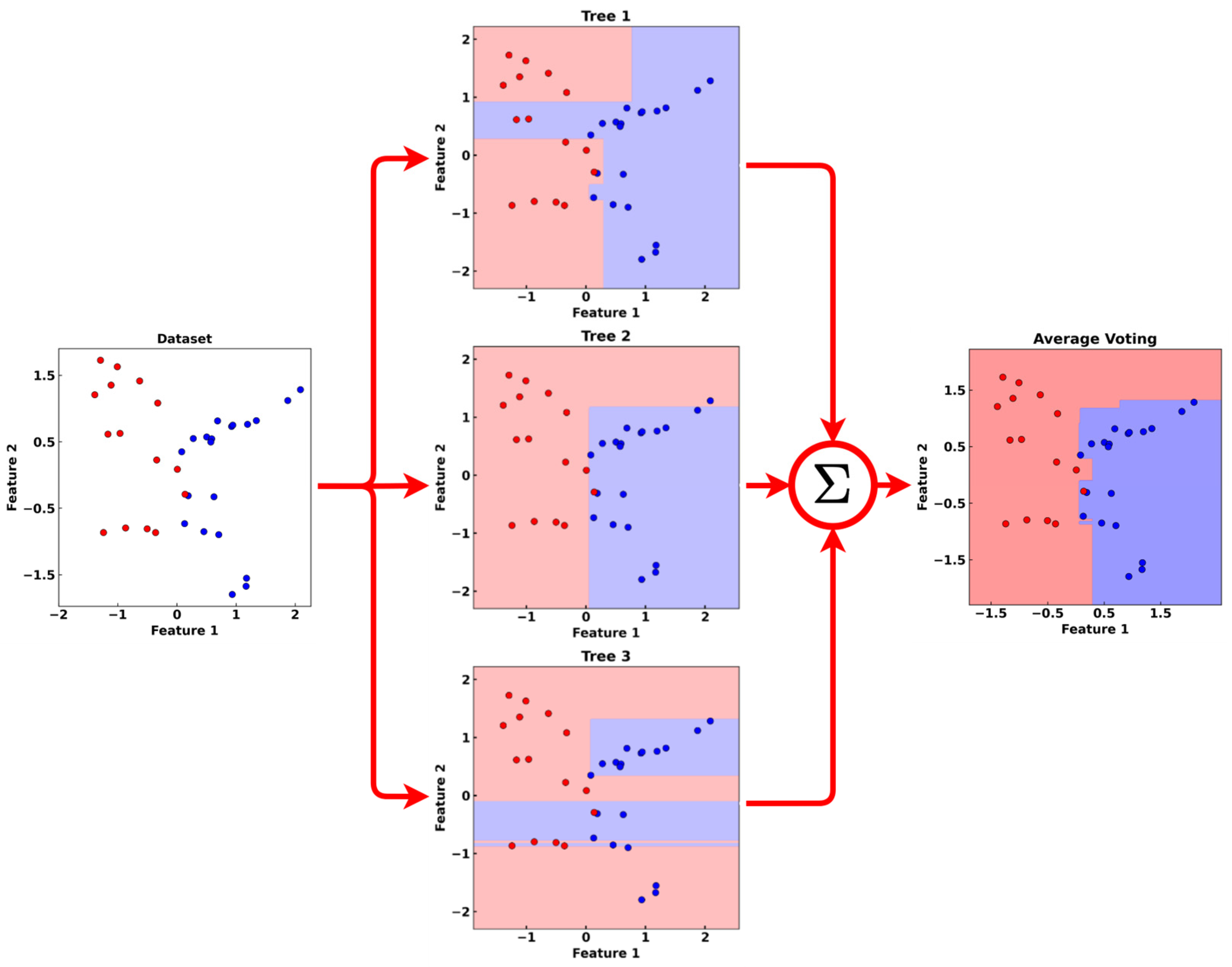
4.1. Random Forest Classifier

Typically, an RFC belongs to the ensemble method category. Ensemble methods can be broadly categorized into three types, including stacking, boosting, and bagging. Bagging methods, such as random forests [47] and Bagging [48,49], aim to create multiple estimators and aggregate their outputs to reduce variance and improve overall performance. In brief, by combining multiple estimators, ensemble methods usually guarantee effective generalization across various data patterns, which in turn enhances the overall predictive accuracy and stability of the models, as shown in Figure 1.

Figure 1 shows the performance of the RFC using three estimators. Individually, the prediction accuracy of each “weak estimator” may not be acceptable due to relatively high errors rates. However, when these three estimators are combined through averaged voting, a different story emerges. As clearly depicted, the accuracy achieved through the ensemble’s averaged voting is significantly improved.

4.2. Multiplayer Perceptron Algorithm (MLP)

The multilayer perceptron (MLP) enhances the capabilities of the ANN model to capture the underlying patterns within complex datasets. Generally, the MLP algorithm consists of a combination of multiple interconnected layers, including input, output, and hidden layers.

In the context of an MLP, the forward pass involves the input data of size $m$ being multiplied by a weight vector $W$ and passed through an activation function $\sigma \left(x\right)$ at each neuron in the hidden layers. The value of each neuron at any layer can be calculated as follows:

$$h^{\left(n\right)}={\sum }_{m=1}^M\left(w_m^{\left(n\right)}.h_m^{\left(n-1\right)}+b^{\left(n\right)}\right)$$

(14)

where $h^{\left(n\right)}$ is the input of the hidden layer $n$, $h^{\left(n-1\right)}$ is the output from the previous layer, $w^{\left(n\right)}$ is the weight matrix, $b^{\left(n\right)}$ is the bias vector, and $M$ is the number of neurons involved in each layer. In the same manner, the estimated output can be computed using the output of the last hidden layer as follows:

$$\widehat{y}=\sigma \left({\sum }_{m=1}^M\left(w_m^{\left(n\right)}.h_m^{\left(n\right)}+b^{\left(n\right)}\right)\right)$$

(15)

where $\widehat{y}$ signifies the estimated output. Once the estimated output is calculated, the error is also computed based on the actual values. By applying the chain rule, the gradient descent with respect to weights and biases is computed, and all weights and biases are updated accordingly, as in (16) and (17):

$$W^{\left(n\right)}=W^{\left(n\right)}-\eta {\displaystyle \frac{\partial \mathcal{L}}{\partial W^{\left(n\right)}}}$$

(16)

$$b^{\left(n\right)}=b^{\left(n\right)}-\eta {\displaystyle \frac{\partial \mathcal{L}}{\partial b^{\left(n\right)}}}$$

(17)

where ${\displaystyle \frac{\partial \mathcal{L}}{\partial W^{\left(n\right)}}}$ and ${\displaystyle \frac{\partial \mathcal{L}}{\partial b^{\left(n\right)}}}$ are the gradients of the loss function for each weight and bias, respectively. In addition to preventing significant and erratic changes in weights and biases, the learning rate (η) is incorporated into the equations.

4.3. Support Vector Classifier (SVC)

In the SVC realm, support vectors refer to points closest to the boundary of the hyperplane, while the margin is the distance between the hyperplane and these support vectors [50,51,52]. This structure is fundamental to the operation of the SVC, as illustrated in Figure 2. The equation defining the hyperplane is given in (18).

$$d\left(x\right)=w^T·x+b$$

(18)

where $x$ signifies the input vector, the weight vector perpendicular to the hyperplane is represented by $W$, and $b$ represents the $y$-axis intercept. Additionally, the width of the decision boundary margin can be determined as in (19).

$$\gamma ={\displaystyle \frac{2}{‖w‖}}$$

(19)

Here, ‖w‖ represents the Euclidean norm of the weight vector.

To address noise, skewness, and irrelevance information associated with data, the concept of a soft-margin SVM was introduced in [53]. Consequently, the margin can be reformulated to optimize this trade-off as follows:

$$\gamma ={\displaystyle \frac{2}{{‖w‖}^2}}+C{\sum }_{i=1}^n{\zeta }_i$$

(20)

where the slack variable (${\zeta }_i$) is introduced to accommodate potential, and the $C$ parameter is the slack penalty. Consecutively, the convex optimization problem for maximizing the margin in the SVC domain can be expressed with the constraint as $y_i\left(w^T·x_i\right)+b \ge 1-{\zeta }_i,$ where ${\zeta }_i \ge 0$. However, due to the inherent nonlinearity, the original dataset ($x_i$) must be projected into a higher-dimensional space ($\varphi \left(x_i\right)$), where a linear boundary can effectively separate the dataset $x_i$. Given the computationally intensity of this process, the deployment of the kernel function becomes crucial, offering an efficient solution to the inner product calculation by using the kernel trick $k(x, x_i)$ = $\varphi \left(x\right)· \varphi \left(x_i\right)$. The most well-known kernel in SVC is the Gaussian kernel, also known as the radial basis function (RBF) kernel, which defines $k(x, x_i)$ as follows [51,52,54]:

$$k\left(x,x_i\right)={ e}^{-\delta {‖x-x_i‖}^2},\mathrm{where} \delta ={\displaystyle \frac{1}{2{\epsilon }^2}}$$

(21)

where $\delta ,$ the user-defined parameter, regulates the flexibility of the decision boundary, and the RBF kernel width is defined using $\epsilon$. Lastly, the standard form of the SVC can be formulated as follows [45,55,56,57,58]:

$$f\left(x\right)=\sum _{i=1}^n\left({\alpha }_i y_i k\left(x, x_i\right)\right)+b$$

(22)

where ${\alpha }_i$ is known as the Lagrange multiplier.

Figure 2. Illustration of the performance of the SVC.

Figure 2. Illustration of the performance of the SVC.

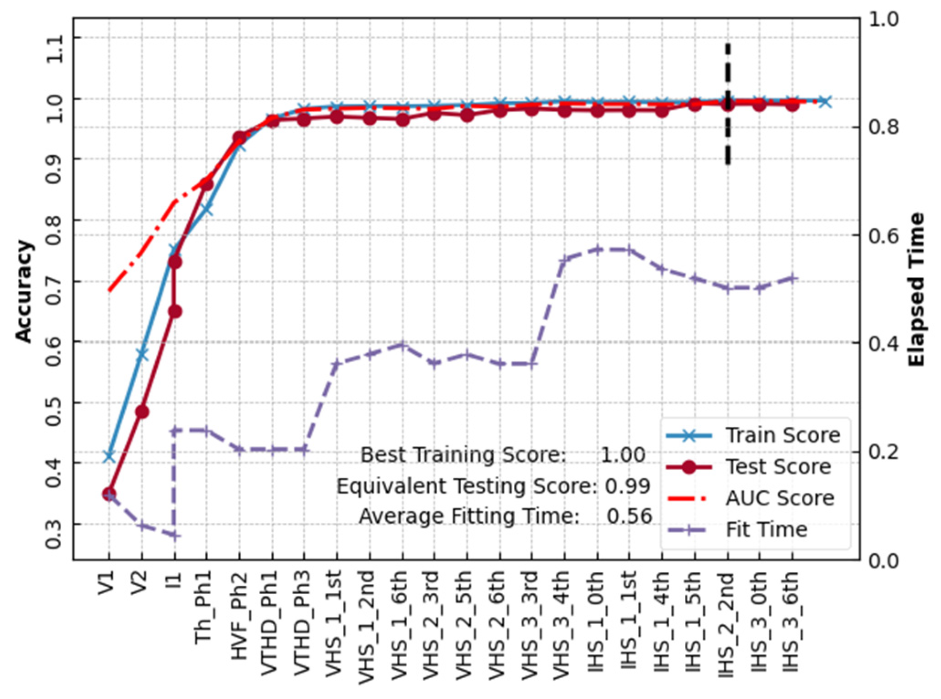
5. Research Methodology

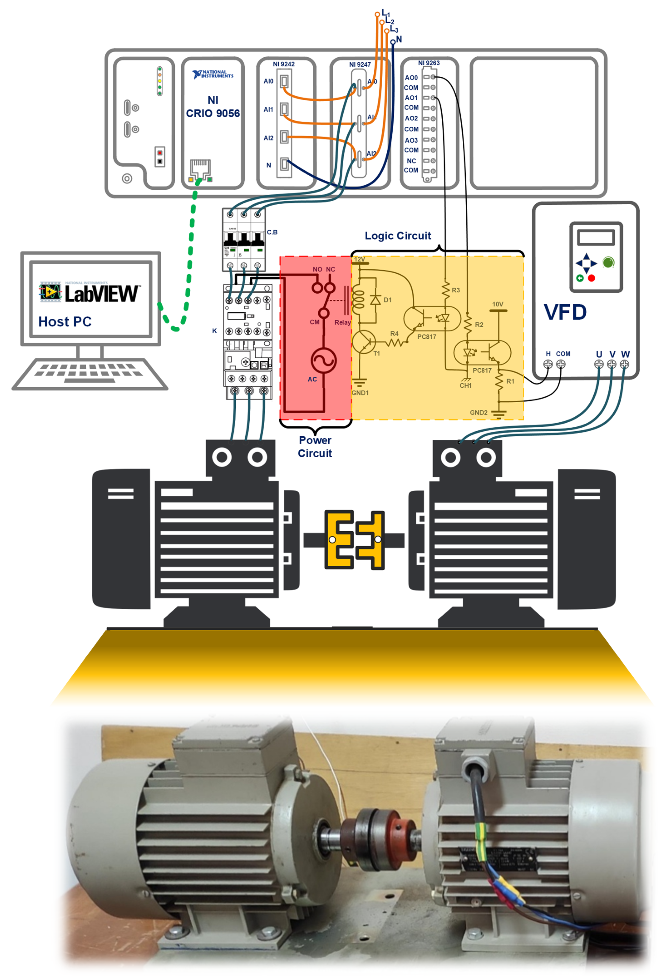
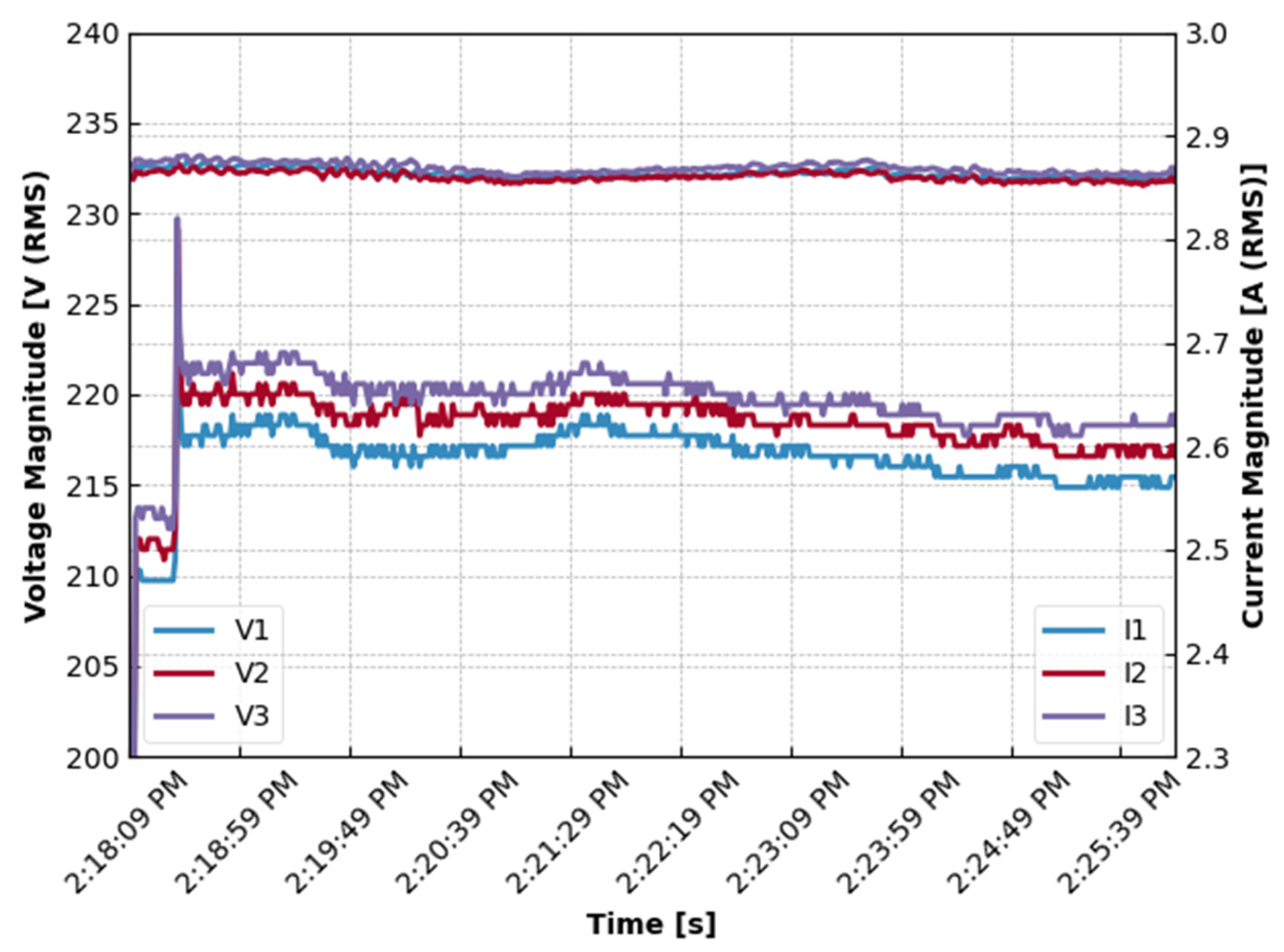
The research methodology is systematically structured to ensure an effective operative assessment of the proposed AHC-based feature selection method in fault diagnosis of IMs, as shown in Figure 3. Initially, data acquisition is conducted using the NI cRIO-9056 embedded controller, which captures three-phase voltage and current signals at the motor terminals with a 5 kHz sampling rate, ensuring high-resolution signal representation. Measurements are collected under diverse operating conditions to provide broad coverage of real-world fault scenarios. It is worth mentioning that each test scenario was conducted for a duration of 10 min to ensure consistency in data acquisition, class distribution balance, and fault pattern development. Nevertheless, the single-phase loss test was limited to 3 min due to the increased thermal stress imposed on the stator insulation, which could compromise machine integrity if exposed for an extended period.

Once the signals are captured, they undergo a preprocessing stage, where a low-pass second-order Butterworth filter is employed to effectively attenuate high-frequency noise while maintaining the integrity of relevant fault-related features. This ensures clean, high-fidelity data, optimizing feature extraction for subsequent analysis. These filtered waveforms form the basis for the feature engineering stage, during which a comprehensive set of candidate features is extracted. Following feature extraction, data cleaning and standardization are initiated. This process comprises outlier detection and removal, and imputation of missing values. Subsequently, all numerical features are normalized using z-score standardization. The resulting dataset is then partitioned into 67 percent for training and 33 percent for testing to facilitate model validation.

Considering the AHC-based feature selection phase, Spearman rank-order correlation coefficients are computed to construct a correlation matrix, from which a dendrogram is generated using Ward’s linkage method. Inconsistency coefficients guide the removal of clusters, ensuring that highly collinear or redundant features are eliminated. The outcome is a reduced feature subset that maximizes discriminative power while mitigating multicollinearity.

Subsequently, hyperparameter optimization is conducted using the Successive Halving Algorithm (SVA) for each classifier. Considering a 5-fold cross-validation framework on the training data, the search space for the RFC included the number of estimators $\in \left\{\mathrm{10,50,100}\right\},$ minimum samples per leaf $\in \{\mathrm{1,5},10\}$, and minimum samples required to split $\in \{\mathrm{2,4},7\}.$ For the SVC with the RBF kernel, the penalty parameter $C \in \left\{\mathrm{1,10,100,1000}\right\}$ and kernel coefficient $\gamma \in \{1e^{-3},1e^{-4},1e^{-5}\}$ were considered. For the multilayer perceptron (ANN), the hidden layer sizes $\in \left\{\right(50,),(100,),(150,\left)\right\}$, L2 regularization penalty $\in \{1e^{-4},1e^{-3},1e^{-2}\}$, while the maximum number of iterations was set to 1000. All experiments were conducted using a fixed random seed of 42 and identical hardware/software (Python 3.11.7; Numpy 1.26.4; Pandas 2.2.1; Scikit-learn 1.4.2; Intel Core i7-9700 CPU; 16 GB RAM) to ensure reproducibility.

Finally, in the fault detection and classification stage, each classifier, trained on the AHC-selected feature subset with optimized hyperparameters, is evaluated using accuracy, precision, recall, and the F1-score. A comparative analysis against random forest-based feature selection and models trained on the full feature set demonstrates that the AHC approach yields superior generalization, higher class-balanced performance, and improved interpretability. The validated models are then prepared for real-time deployment, enabling continuous condition monitoring and automated alert generation in industrial environments. Those steps are summarized in Figure 3.

Experimental Setup

Figure 4 offers a visual illustration of the assembled validation test rig at the Energy Efficiency and Sustainability Technology Laboratory, Faculty of Technology and Education, Suez University. The setup included two mechanically coupled IMs of identical size, each rated at 1.1 kW, 220 V/400 V Δ/Y, and 1410 RPM. The motor under investigation was subjected to various fault conditions, while the second motor was connected to a variable frequency (V/F) drive, serving as a mechanical load to ensure controlled operating conditions and accurate fault replication.

Table 1. Summary of operating scenarios, fault types, and experimental conditions.

Operating Scenario	Description	Scenario Duration	Operating Scenario	Description	Scenario Duration
No-load	Motor running under no-load condition.	10 min	Rear Defect (5 mm)	Motor at full load with a 5 mm defect in the outer race of the rear bearing.	10 min
Full-load	Motor running at full load, drawing a current of 2.73 A.		Front and Rear Defect (2 mm)	Motor at full load with a 2 mm defect in the outer races of both the front and rear bearings.
Front Defect (2 mm)	Motor at full load with a 2 mm defect in the outer race of the front bearing.		Front and Rear Defect (5 mm)	Motor at full load with a 5 mm defect in the outer races of both the front and rear bearings.
Front Defect (5 mm)	Motor at full load with a 5 mm defect in the outer race of the front bearing.		Phase loss fault	Motor operating with a single-phase open fault, where one phase is disconnected during operation.	3 min
Rear Defect (2 mm)	Motor at full load with a 2 mm defect in the outer race of the rear bearing.

provides a comprehensive summary of the faults introduced to the motor during the experimental tests, detailing the specific fault types, severity levels, and corresponding operating conditions to ensure a thorough analysis of the diagnostic methodology. As clearly seen from Table 1, the study focuses primarily on bearing faults, given their prevalence in induction motors [11,24,27], and includes a single-phase loss fault to examine electrical imbalance effects [48,49]. These selections ensure relevance to industrial applications, where bearing degradation and phase loss are common failure modes affecting reliability and operational efficiency.

The NI-9247 c-series current input module, the NI-9242 c-series voltage input module, and the NI-9263 analog output module were all connected through the chassis of the NI-cRIO 9056 controller (Austin, TX, USA). This setup utilized the Xilinx Artix-7 75T FPGA processor (Xilinx, Inc., San Jose, CA, USA), which managed the data acquisition and control tasks at a 5 kHz sampling rate. The extracted features were then delivered instantaneously to a real-time floating-point processor, an Intel Atom E3805, which handled communication with the centralized server. The captured three-phase RMS values of the voltage and current phasors are illustrated in Figure 5.

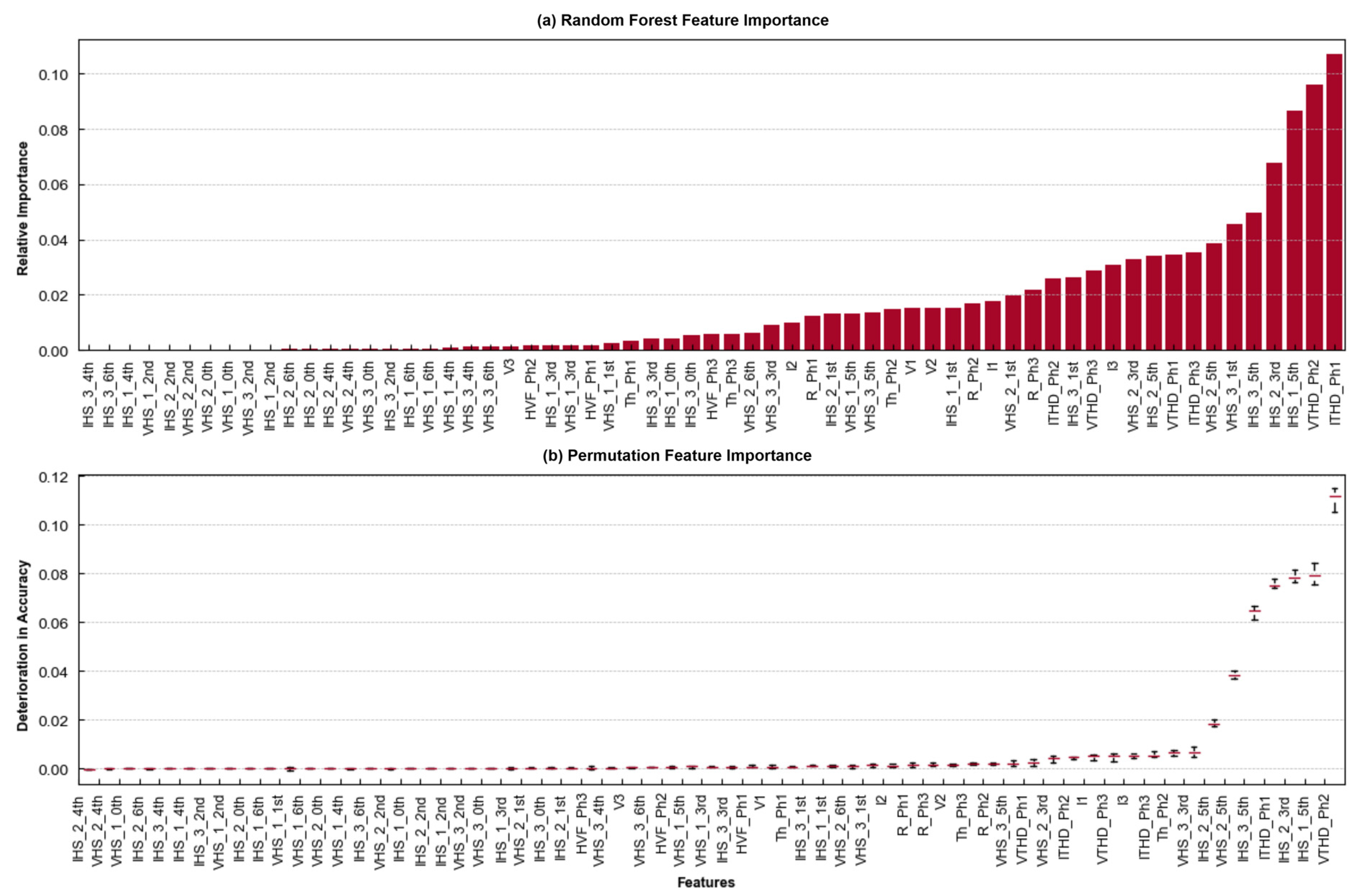
6. Exploration of Findings

Figure 6 presents a comprehensive summary of the harmonic profiles for voltage and current phases. The analysis of the harmonic spectra reveals that, across all three phases, the first harmonic magnitudes of voltage and current remain relatively stable in most cases, except for the current spectrum under the Single-Phase Fault condition. As clearly observed, Single-Phase Fault on phase 2 drives phase 2 current to zero. The spectrum thus collapses (bars near 10⁻⁴ A). Meanwhile, the fundamental harmonics in the other phases show a relative increase, and the non-fundamental harmonics exhibit noticeable spikes in magnitude. On the other hand, in all phases, the third and fifth harmonics consistently dominate the non-fundamental components with relatively small differences under different scenarios. Notably, THD for voltage (VTHD) remains below 2.5 percent in healthy and minor defect scenarios but exceeds 2 percent under a front defect of 5 mm and reaches up to 2.3 percent in phase 2 only. Current THD (ITHD) remains under 3 percent for all defects but spikes to 27 percent in phase 2 under “Single-Phase Fault,” clearly signaling severe unbalance [35].

Comparing HVF to VTHD, the HVF values (10⁻³–10⁻² percent) are much smaller but still reliably track relative distortions, as can be clearly seen in Figure 6. Overall, the harmonic profiles, along with the THD and HVF metrics, capture subtle variations across different cases; these variations form the basis upon which the adopted classifier accurately predicts the actual states of the IM.

On another note, to ensure a comprehensive evaluation, the three previously mentioned estimators (RFC, ANN, and SVC) are trained and tested under different scenarios. The effectiveness of the presented method of feature selection against the well-stablished method (feature importance trait of random forest classifier) has been evaluated. As discussed earlier, the hyperparameter of the adopted classifiers were optimized using SVA. Consequently, the SVC employed an RBF kernel with a penalty parameter $C=1000$ and kernel coefficient $\gamma =0.001$. The MLP-based ANN was configured with one hidden layer of 150 neurons, an L2 regularization term of $\alpha =0.0001,$ and a maximum of 1000 iterations. For the RFC, the model used 10 decision trees, with a minimum of five samples per leaf and a minimum of two samples required to split an internal node. These settings were selected to balance model complexity and generalization performance across varying fault diagnosis scenarios.

In a different context, to recognize the importance of feature selection,

Table 2. Performance analysis of RFC, ANN, and SVC estimators using the complete feature set.

Metrics	Precision			Recall			F1-Score
Classifier	RFC	ANN	SVC	RFC	ANN	SVC	RFC	ANN	SVC
No-load	1.000	1.000	0.868	1.000	1.000	1.000	1.000	1.000	0.929
Full-load	0.997	0.965	1.000	0.995	0.768	0.000	0.996	0.855	0.000
Front Defect (2 mm)	1.000	0.996	1.000	0.999	0.955	0.000	0.999	0.975	0.000
Front Defect (5 mm)	1.000	0.995	1.000	0.997	0.997	0.000	0.999	0.996	0.000
Rear Defect (2 mm)	0.994	0.680	1.000	0.986	0.165	0.000	0.990	0.266	0.000
Rear Defect (5 mm)	1.000	0.813	1.000	0.982	0.644	0.000	0.991	0.718	0.000
Front and Rear Defect (2 mm)	1.000	0.992	1.000	0.996	0.978	0.000	0.998	0.985	0.000
Front and Rear Defect (5 mm)	0.999	0.870	1.000	0.983	0.781	0.000	0.991	0.823	0.000
Single-Phase Fault	0.970	0.987	0.957	0.985	0.900	0.605	0.977	0.941	0.741
micro avg	0.997	0.946	0.885	0.992	0.797	0.154	0.995	0.865	0.263
macro avg	0.996	0.922	0.981	0.991	0.799	0.178	0.993	0.840	0.186
weighted avg	0.997	0.920	0.982	0.992	0.797	0.154	0.995	0.838	0.153

demonstrates the performance of the three selected classifiers using all 63 features extracted from voltage and current signals. Various performance measures, including accuracy, precision, recall, and the F1 score, were used to evaluate the effectiveness of each estimator, as reported in Table 2. The performance of the SVC was the worst, with an accuracy of approximately 15.43%. This unsatisfactory performance can be directly attributed to the classifier’s sensitivity to irrelevant and noisy features, which adversely affected its ability to generalize from the data. Additionally, the SVC required approximately 66 s for training. On the contrary, the ANN demonstrated significantly better performance compared to the SVC, achieving an accuracy of 77.34%, albeit still being disrupted by the presence of noisy or irrelevant features. However, the training time for the ANN was notably longer, at approximately 215 s. The longer fitting time of the ANN reflects the complexity and computational demands of the model. The RFC outperformed both the SVC and the ANN. The classifier achieved an accuracy of 99.192%. Given the inherent structure of the RFC, its superior performance is expected and logically acceptable. Notably, the RFC also had the shortest training time of just 0.82 s.

Figure 7 presents a detailed analysis of feature significance by comparing the results obtained from the RFC and a permutation analysis approach. The features are sorted in ascending order based on their importance, as determined by the RFC, as shown in Figure 7a. In contrast, Figure 7b depicts the permutation analysis of the same features. The permutation analysis assesses the impact of shuffling each feature on model accuracy. Together, these visualizations provide a comprehensive understanding of feature significance. Notably, when focusing on the most important features, both methods consistently identify the same five dominant features: the THD of phase 1 current (ITHD_ph1), THD of phase 2 voltage (VTHD_Ph2), fifth harmonic of phase 1 current (IHS_1_5th), the third harmonic of phase 2 current (IHS_2_3rd), and the fifth harmonic of phase 3 current (IHS_3_5th), albeit with slight variations in their order. Despite this consistency, permutation analysis reveals that four of these features exhibit an average reduction in accuracy of approximately 0.07%, while only one feature shows a more tangible deterioration in accuracy of 0.12%. In contrast to the RFC’s feature importance, permutation analysis reveals the insignificance of other features on the overall performance of the predictive model, which emphasizes the issue of multicollinearity among correlated datasets. This redundancy underscores the need for more intelligent feature selection algorithms.

To thoroughly investigate the presented methodology, the following subsections cover three cases. The first case evaluates the performance of three classifiers, SVC, ANN, and RFC, using the top twenty-three dominant features identified by the RF feature importance metric, while the second case reports the performance of these classifiers using the twenty-three features selected by the AHC algorithm. Lastly, the third case involves a comparative analysis based on feature importance.

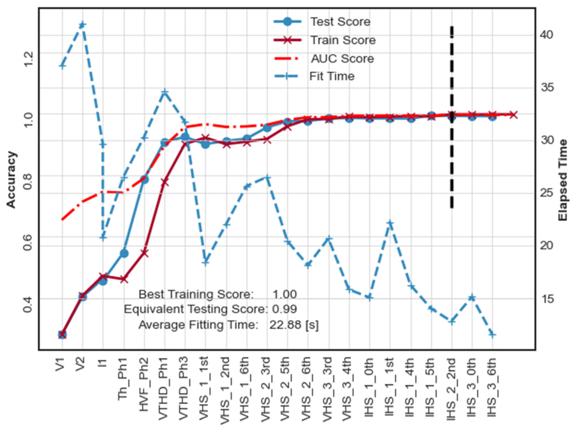
6.1. Case No. 1: RF-Based Feature Selection

Following the same procedures, the first twenty-three features, as reported in Figure 7a, are employed to train the three classifiers. The results are reported in

Table 3. Performance analysis of RFC, ANN, and SVC estimators using RF-based feature selection.

Metrics	Precision			Recall			F1-Score
Classifier	RFC	ANN	SVC	RFC	ANN	SVC	RFC	ANN	SVC
No-load	1.000	0.997	0.999	1.000	1.000	1.000	1.000	0.999	0.999
Full-load	0.992	0.980	0.974	0.995	0.995	0.995	0.994	0.987	0.984
Front Defect (2 mm)	1.000	0.997	0.996	0.996	1.000	0.993	0.998	0.999	0.994
Front Defect (5 mm)	1.000	1.000	0.997	0.997	0.997	0.997	0.999	0.999	0.997
Rear Defect (2 mm)	0.997	0.996	0.940	0.987	0.991	0.920	0.992	0.994	0.930
Rear Defect (5 mm)	0.997	0.959	0.947	0.992	0.996	0.968	0.994	0.977	0.957
Front and Rear Defect (2 mm)	1.000	0.997	0.996	0.996	0.999	1.000	0.998	0.998	0.998
Front and Rear Defect (5 mm)	0.999	0.997	0.996	0.983	0.947	0.964	0.991	0.971	0.979
Single-Phase Fault	0.976	0.990	0.963	0.976	0.945	0.936	0.976	0.967	0.949
micro avg	0.997	0.990	0.980	0.992	0.988	0.978	0.995	0.989	0.979
macro avg	0.996	0.990	0.978	0.991	0.986	0.975	0.993	0.988	0.977
weighted avg	0.997	0.990	0.980	0.992	0.988	0.978	0.995	0.989	0.979

. As can be clearly seen, the performance of all three classifiers improved significantly. The accuracy of the SVC increased to 96.75%, with a fitting time of 5.30 s. This remarkable improvement highlights the crucial effect of removing irrelevant and noisy features, which allows the SVC to generalize much more effectively. Similarly, the ANN’s average accuracy increased to 98.68%, with a remarkable reduction in fitting time of 8.30 s. The random forest classifier’s average accuracy slightly improved to 99.24%, with a fitting time of 0.72 s. This minor improvement in accuracy, together with the slight reduction in fitting time, confirms the robustness and efficiency of the RFC.

Furthermore, Table 3 demonstrates that the RFC consistently achieved the highest precision, recall, and F1-scores, particularly excelling in detecting complex faults, including those involving simultaneous defects in both the front and rear bearings. The ANN followed closely, offering competitive F1-scores but with slightly reduced precision and recall in some fault cases. In contrast, the SVC showed a noticeable drop in recall, especially for rear defects (as low as 0.920) and single-phase faults (0.936), which indicates limited sensitivity to these conditions. Average metrics further confirmed the RFC’s robustness and generalization capabilities compared to those of other classifiers, with the macro and weighted F1-scores reaching 0.993 and 0.995, respectively. These results underscore the RFC’s reliability for multiclass fault diagnosis in IMs, while the ANN remains a viable alternative. In contrast, the SVC appears less suitable without further optimization.

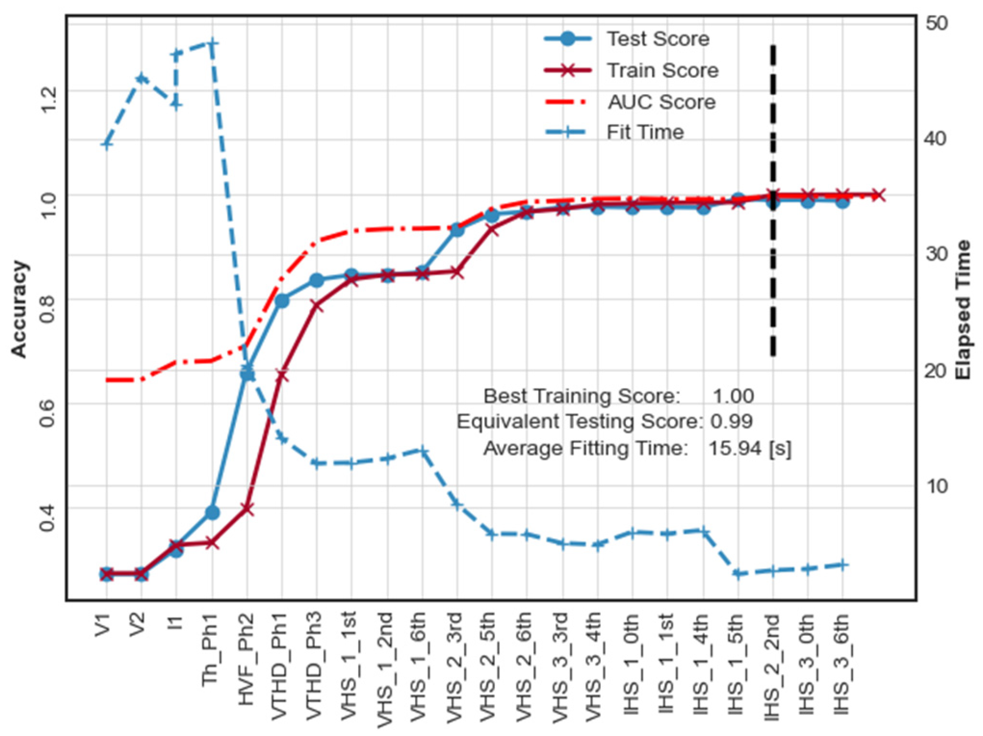
6.2. Case No. 2: AHC-Based Feature Selection

The dendrogram based on the Spearman correlation matrix is presented in Figure 8 to evaluate the interrelationships among all features and to assess their influence on classifier performance. The dendrogram in Figure 8 highlights how features are inherently grouped into four distinct clusters. Each cluster shares common information among the features it contains. Additionally, Figure 8 is color-coded: features identified as important by the RF algorithm are colored blue, features deemed important by both the RF and the suggested algorithm are highlighted in red, and those identified exclusively by the proposed algorithm are marked in purple. Notably, RF-based methods tend to select features with high correlations or shorter distances in hierarchical clustering terms. However, AHC-based feature selection selects a representative set of features from each cluster. The suggested approach ensures that all clusters are represented and considered. Such an approach should better preserve unique information while effectively mitigating issues of multicollinearity. The performance of the features selected by the AHC algorithm is reported in

Table 4. Performance analysis of RFC, ANN, and SVC estimators using AHC-based feature selection.

Metrics	Precision			Recall			F1-Score
Classifier	RFC	ANN	SVC	RFC	ANN	SVC	RFC	ANN	SVC
No-load	1.000	1.000	1.000	1.000	1.000	1.000	1.000	1.000	1.000
Full-load	0.996	0.992	0.997	0.994	0.991	0.992	0.995	0.992	0.995
Front Defect (2 mm)	1.000	0.997	0.997	0.999	0.999	0.993	0.999	0.998	0.995
Front Defect (5 mm)	1.000	0.999	1.000	0.997	0.997	0.996	0.999	0.998	0.998
Rear Defect (2 mm)	0.996	0.997	0.994	0.990	0.991	0.989	0.993	0.994	0.991
Rear Defect (5 mm)	0.994	0.989	0.985	0.968	0.989	0.981	0.981	0.989	0.983
Front and Rear Defect (2 mm)	1.000	1.000	0.999	0.992	0.997	0.993	0.996	0.999	0.996
Front and Rear Defect (5 mm)	0.989	0.992	0.989	0.981	0.986	0.985	0.985	0.989	0.987
Single-Phase Fault	0.972	0.973	0.964	0.964	0.991	0.985	0.968	0.982	0.974
micro avg	0.996	0.995	0.994	0.989	0.994	0.991	0.992	0.994	0.992
macro avg	0.994	0.993	0.992	0.987	0.993	0.990	0.991	0.993	0.991
weighted avg	0.996	0.995	0.994	0.989	0.994	0.991	0.992	0.994	0.992

, in which the same performance metrics as those used in Case No. 1 are employed.

As reported in Table 4, all three classifiers exhibited significant improvements in their performance. Notably, the accuracy of the SVC increased by approximately 2.03%, increasing from 96.75% in Case No. 1 to 98.724%, with the fitting time reduced to just 4.32 s. This enhancement underscores the representativeness of the features selected by AHC, which is allowing the SVC to generalize more effectively across diverse operational conditions. Similarly, the ANN’s average accuracy increased to 99.257%, with a fitting time of 14.33 s, compared to 98.68% achieved in Case No. 1. The improvement in accuracy indicates a more efficient learning process, albeit with a slight increase in training time compared to the RF-based selection. Conversely, the RFC exhibited a slight decline in its average accuracy, dropping to 98.869%, while achieving a fitting time of just 0.74 s.

Furthermore, the application of AHC for feature selection resulted in measurable performance improvements, particularly for the ANN and SVC. In the AHC-based feature set, the ANN achieved a macro-averaged F1-score of 0.993 and a weighted average F1-score of 0.994, both higher than in the RFC-based feature set (0.988 and 0.989, respectively). Similarly, the SVC improved its macro average F1-score from 0.977 to 0.991 and weighted average from 0.979 to 0.992.

For complex classes such as rear defect: 5 mm, the ANN improved its F1-score from 0.977 to 0.989, and the SVC from 0.957 to 0.983. In the challenging Single-Phase Fault class, the ANN’s F1-score increased from 0.967 to 0.982, and the SVC’s from 0.949 to 0.974. Meanwhile, the RFC showed stable performance, with only marginal changes, which indicates its robustness but a limited benefit from AHC. Importantly, all classifiers achieve perfect scores for the no-load state, confirming excellent generalization in identifying healthy conditions. The macro and weighted averages confirm that AHC-based feature selection significantly reduces performance variability, enhances generalization, and strengthens fault discrimination, demonstrating its competitive advantage over RFC-based feature importance.

Although the accuracy reduction of the RFC is minor, the marginal increase in training time indicates that the RFC still benefits from the refined feature selection process, albeit to a lesser extent compared to the other classifiers. The robustness of the RFC remains evident in both cases; however, the results suggest that the features introduced through AHC may be advantageous for the SVC and ANN but could pose minor challenges to the RFC’s optimization.

Briefly, Figure 9 provides a comparative analysis of accuracy and fitting time across the three classifiers. The analysis reveals that implementing feature selection strategies significantly enhances classifier performance. Although using all 63 features achieves a high accuracy of 99.192% for RFC, the ANN demonstrates only moderate performance at 77.338%, while the SVC records the poorest accuracy at just 15.426%. However, adopting either RF- or AHC-based feature selection significantly enhances the overall accuracy of all classifiers while simultaneously reducing fitting time. AHC-based feature selection outperforms RF for the ANN and SVC, achieving accuracies of 99.257% and 98.724%, respectively. Furthermore, AHC provides a balance between high accuracy and reduced fitting time, making it more efficient for computationally intensive models.

6.3. Case No. 3: Comparative Analysis of Classifiers’ Performance Considering Feature Selection Algorithms

6.3.1. Random Forest Classifier (RFC)

Figure 10 and Figure 11 depict the RFC’s performance with two different feature subsets, derived from AHC and RF, respectively. These figures summarize the sensitivity analysis conducted to assess the impact of each feature subset. The investigation primarily aims to determine the capability of feature selection algorithms to identify features that effectively represent the entire population. This is achieved by incrementally adding one feature at a time and evaluating the impact of each addition on the overall performance and generalizability of the model.

Considering the trade-off between accuracy and the number of features, both figures consistently demonstrate significant improvements in estimator performance (training score, testing score, and AUC score) as more features are added. Notably, the training and testing scores displayed in the figures are very similar to each other, which indicates effective fine-tuning of RFC hyperparameters. This closeness highlights minimal overfitting and strengthens model generalizability. The highest training score for both methods is 100%, and the corresponding testing score is also 99%. The AUC score also closely follows the testing score, indicating consistent performance. However, the superiority of the developed method for feature selection based on AHC is apparent in the early appearance of a vertical black dashed line in Figure 10. This line denotes the point at which the model achieves its highest performance score, which occurs with fewer features compared to the RF-based method. The superiority is further supported by the relatively early stabilization of both testing and training curves in Figure 10 compared with the RF-based method shown Figure 11. On the other hand, the fitting time, as indicated by the dashed purple lines in both figures, exhibits a non-linear insignificant increase as the number of features increases, which indicates a corresponding increase in model complexity. However, the average fitting time associated with RF- and AHC-based feature selection remains relatively the same, demonstrating a comparable computational burden.

6.3.2. Artificial Neural Networks (ANNs)

Similarly, Figure 12 and Figure 13 illustrate the performance of the ANN estimator using features selected by AHC and RF, respectively. Both instances of the ANN estimator exhibit high training scores (100% and 99%, respectively) and equivalent test scores of 99%, which indicates excellent performance on the training set and the ability to generalize well to unseen data. However, the test score for the AHC-based estimator exhibits fluctuations at the initial stage, before stabilizing and aligning with the training score after a certain number of features are added. This fluctuation can be attributed to the hyperparameter optimization process, which is specifically tuned to the features selected by the random forest model. Notably, the AHC-based ANN instance, Figure 12, achieves high accuracy with a comparatively smaller number of selected features, as indicated by the vertical black line. Additionally, both algorithms show a gradual rise in the AUC score as more features are added.

Nevertheless, the fitting time presents a contrasting narrative. The AHC-based ANN model shows significant variation, with an average fitting time of 22.88 s. In contrast, the RF-based ANN model, though slightly fluctuating, consistently achieves faster fitting times, averaging 12.33 s. This increase can be attributed to the iterative nature of the backpropagation algorithm, which demands extensive weight adjustments across multiple layers, leading to higher computational overhead.

The AHC-selected features, while highly discriminative, contribute to this complexity by increasing the number of optimized parameters during training. However, in static operational environments, where model updates are infrequent, the ANN remains a highly reliable choice for fault diagnosis, offering superior classification accuracy despite the increased computational cost.

6.3.3. Support Vector Machines (SVC)

Similarly, as clearly illustrated in Figure 14, the rapid achievement of optimal convergence after only 15 features strongly suggests that AHC-based feature selection has effectively identified the optimal subset. Conversely, Figure 15 indicates that RF-based feature selection requires a slightly larger number of features to compensate for the lack of informative features and to achieve comparable levels of accuracy and stability. Although the initial fitting time is high (indicated by the blue dashed line) due to the model’s difficulty in converging with a limited number of features, both algorithms show a steady decrease in fitting time as additional features are added. The average fitting time for the AHC-based algorithm is approximately 15.94 s, while the RF-based algorithm requires around 19.03 s. The AHC approach reaches its minimum fit time of approximately 2 s, consistently outperforming the RF-based instance. This behavior suggests that AHC-based feature selection may lead to a more stable and efficient training process.

7. Conclusions

In this paper, the agglomerative hierarchical clustering (AHC)–based feature selection algorithm for induction motor (IM) fault diagnosis is investigated. The performance of AHC is compared with a random forest (RF)–based feature importance approach. Across all experiments, AHC consistently yields a compact, highly discriminative feature subset that mitigates multicollinearity and improves model generalizability. A total of 63 extracted features are derived from the voltage and current signals captured from the motor terminals.

By employing all 63 extracted features, the RF classifier (RFC) achieved an accuracy of 99.192% with minimal training time (0.82 s). In contrast, the Support Vector Classifier (SVC) and the multilayer perceptron (ANN) attained only 15.426% and 77.338% accuracy, respectively, due to their sensitivity to redundant features. Incorporating RF-based feature selection (a subset of 23 features) noticeably improved classification: SVC increased to 96.75% (5.30 s), ANN to 98.68% (8.32 s), and RFC to 99.24% (0.72 s). These performance enhancements underscore the importance of removing irrelevant or noisy inputs, but do not guarantee that the selected subset contains the most discriminative features. On the other hand, AHC-based selection further enhanced performance by capturing cluster-representative harmonic features. Using 23 AHC-selected features, SVC achieved an accuracy of 98.724% in 4.32 s, and ANN reached 99.257% in 14.33 s, each outperforming their RF-selected counterparts. Although RFC′s accuracy slightly declined to 98.869% with AHC, its training time remained low (0.74 s), which highlights the inherent robustness of RFC. Moreover, sensitivity analyses confirmed that AHC attained optimal performance with fewer features, while RF required additional features to achieve similar accuracy levels.

These findings demonstrate that AHC effectively mitigates multicollinearity by grouping correlated harmonics and selecting representative features. Consequently, AHC enhances classification accuracy, particularly for computationally demanding models such as SVC and ANN, while maintaining computational efficiency. Future work should explore scalability to larger motor systems and the integration of time-frequency features, such as wavelet coefficients, to further improve diagnostic robustness under non-stationary conditions.

References

1. Saberi, A.N.; Belahcen, A.; Sobra, J.; Vaimann, T. LightGBM-Based Fault Diagnosis of Rotating Machinery under Changing Working Conditions Using Modified Recursive Feature Elimination. IEEE Access 2022, 10, 81910–81925. [Google Scholar] [CrossRef]
2. Hou, J.; Wu, Y.; Ahmad, A.S.; Gong, H.; Liu, L. A Novel Rolling Bearing Fault Diagnosis Method Based on Adaptive Feature Selection and Clustering. IEEE Access 2021, 9, 99756–99767. [Google Scholar] [CrossRef]
3. Saucedo-Dorantes, J.J.; Jaen-Cuellar, A.Y.; Delgado-Prieto, M.; Romero-Troncoso, R.D.J.; Osornio-Rios, R.A. Condition Monitoring Strategy Based on an Optimized Selection of High-Dimensional Set of Hybrid Features to Diagnose and Detect Multiple and Combined Faults in an Induction Motor. Measurement 2021, 178, 109404. [Google Scholar] [CrossRef]
4. Xue, S.; Hou, Y.; Mi, J.; Zhou, C.; Xiang, T.; He, W.; Wu, D.; Huang, W. Induction Motor Failure Identification Based on Multiscale Acoustic Entropy Feature Selection and Hierarchical Adaptive Neuro-Fuzzy Inference System With Localized Recurrent Input. IEEE Sens. J. 2023, 23, 30821–30834. [Google Scholar] [CrossRef]
5. Lee, C.-Y.; Le, T.-A.; Chien, W.-L.; Hsu, S.-C. Application of Symmetric Uncertainty and Emperor Penguin—Grey Wolf Optimisation for Feature Selection in Motor Fault Classification. IET Electr. Power Appl. 2024, 18, 1107–1121. [Google Scholar] [CrossRef]
6. Islam, R.; Khan, S.A.; Kim, J.-M. Discriminant Feature Distribution Analysis-Based Hybrid Feature Selection for Online Bearing Fault Diagnosis in Induction Motors. J. Sens. 2016, 2016, 7145715. [Google Scholar] [CrossRef]
7. Gangsar, P.; Bajpei, A.R.; Porwal, R. A Review on Deep Learning Based Condition Monitoring and Fault Diagnosis of Rotating Machinery. Noise Vib. Worldw. 2022, 53, 550–578. [Google Scholar] [CrossRef]
8. Hsu, S.; Lee, C.; Fang Wu, W.; Lee, C.; Jiang, J. Machine Learning-Based Online Multi-Fault Diagnosis for IMs Using Optimization Techniques with Stator Electrical and Vibration Data. IEEE Trans. Energy Convers. 2024, 39, 2412–2424. [Google Scholar] [CrossRef]
9. Jigyasu, R.; Shrivastava, V.; Singh, S. Deep Optimal Feature Extraction and Selection-Based Motor Fault Diagnosis Using Vibration. Electr. Eng. 2024, 106, 6339–6358. [Google Scholar] [CrossRef]
10. Jigyasu, R.; Shrivastava, V.; Singh, S. Hybrid Multi-Model Feature Fusion-Based Vibration Monitoring for Rotating Machine Fault Diagnosis. J. Vib. Eng. Technol. 2024, 12, 2791–2810. [Google Scholar] [CrossRef]
11. Buchaiah, S.; Shakya, P. Bearing Fault Diagnosis and Prognosis Using Data Fusion Based Feature Extraction and Feature Selection. Measurement 2022, 188, 110506. [Google Scholar] [CrossRef]
12. Yadav, S.; Patel, R.K.; Singh, V.P. Multiclass Fault Classification of an Induction Motor Bearing Vibration Data Using Wavelet Packet Transform Features and Artificial Intelligence. J. Vib. Eng. Technol. 2023, 11, 3093–3108. [Google Scholar] [CrossRef]
13. Eddine Cherif, B.D.; Seninete, S.; Defdaf, M. A Novel, Machine Learning-Based Eature Extraction Nethod for Detecting and Localizing Bearing Component Defects. Metrol. Meas. Syst. 2022, 29, 333–346. [Google Scholar] [CrossRef]
14. Jalayer, M.; Orsenigo, C.; Vercellis, C. Fault Detection and Diagnosis for Rotating Machinery: A Model Based on Convolutional LSTM, Fast Fourier and Continuous Wavelet Transforms. Comput. Ind. 2021, 125, 103378. [Google Scholar] [CrossRef]
15. Panigrahy, P.S.; Chattopadhyay, P. Tri-Axial Vibration Based Collective Feature Analysis for Decent Fault Classification of VFD Fed Induction Motor. Measurement 2021, 168, 108460. [Google Scholar] [CrossRef]
16. Panigrahy, P.S.; Santra, D.; Chattopadhyay, P. Decent Fault Classification of VFD Fed Induction Motor Using Random Forest Algorithm. Artif. Intell. Eng. Des. Anal. Manuf. 2020, 34, 492–504. [Google Scholar] [CrossRef]
17. Mari, S.; Bucci, G.; Ciancetta, F.; Fiorucci, E.; Fioravanti, A. Impact of Measurement Uncertainty on Fault Diagnosis Systems: A Case Study on Electrical Faults in Induction Motors. Sensors 2024, 24, 5263. [Google Scholar] [CrossRef]
18. Singh, M.; Shaik, A.G. Faulty Bearing Detection, Classification and Location in a Three-Phase Induction Motor Based on Stockwell Transform and Support Vector Machine. Measurement 2019, 131, 524–533. [Google Scholar] [CrossRef]
19. Lee, C.-Y.; Hung, C.-H.; Le, T.-A. Intelligent Fault Diagnosis for BLDC With Incorporating Accuracy and False Negative Rate in Feature Selection Optimization. IEEE Access 2022, 10, 69939–69949. [Google Scholar] [CrossRef]
20. Lee, C.-Y.; Ou, H.-Y. Induction Motor Multiclass Fault Diagnosis Based on Mean Impact Value and PSO-BPNN. Symmetry 2021, 13, 104. [Google Scholar] [CrossRef]
21. Lee, C.-Y.; Zhuo, G.-L. Effective Rotor Fault Diagnosis Model Using Multilayer Signal Analysis and Hybrid Genetic Binary Chicken Swarm Optimization. Symmetry 2021, 13, 487. [Google Scholar] [CrossRef]
22. de las Morenas, J.; Moya-Fernández, F.; López-Gómez, J.A. The Edge Application of Machine Learning Techniques for Fault Diagnosis in Electrical Machines. Sensors 2023, 23, 2649. [Google Scholar] [CrossRef] [PubMed]
23. Zhukovskiy, Y.; Buldysko, A.; Revin, I. Induction Motor Bearing Fault Diagnosis Based on Singular Value Decomposition of the Stator Current. Energies 2023, 16, 3303. [Google Scholar] [CrossRef]
24. Khan, M.A.; Asad, B.; Kudelina, K.; Vaimann, T.; Kallaste, A. The Bearing Faults Detection Methods for Electrical Machines—The State of the Art. Energies 2023, 16, 296. [Google Scholar] [CrossRef]
25. Kudelina, K.; Asad, B.; Vaimann, T.; Rassõlkin, A.; Kallaste, A.; Van Khang, H. Methods of Condition Monitoring and Fault Detection for Electrical Machines. Energies 2021, 14, 7459. [Google Scholar] [CrossRef]
26. Kumar, R.R.; Andriollo, M.; Cirrincione, G.; Cirrincione, M.; Tortella, A. A Comprehensive Review of Conventional and Intelligence-Based Approaches for the Fault Diagnosis and Condition Monitoring of Induction Motors. Energies 2022, 15, 8938. [Google Scholar] [CrossRef]
27. Zhang, S.; Zhang, S.; Wang, B.; Habetler, T.G. Deep Learning Algorithms for Bearing Fault Diagnosticsx—A Comprehensive Review. IEEE Access 2020, 8, 29857–29881. [Google Scholar] [CrossRef]
28. Marmouch, S.; Aroui, T.; Koubaa, Y. Statistical Neural Networks for Induction Machine Fault Diagnosis and Features Processing Based on Principal Component Analysis. IEEJ Trans. Electr. Electron. Eng. 2021, 16, 307–314. [Google Scholar] [CrossRef]
29. Lee, C.-Y.; Lin, W.-C. Induction Motor Fault Classification Based on ROC Curve and T-SNE. IEEE Access 2021, 9, 56330–56343. [Google Scholar] [CrossRef]
30. Nayana, B.R.; Geethanjali, P. Analysis of Statistical Time-Domain Features Effectiveness in Identification of Bearing Faults from Vibration Signal. IEEE Sens. J. 2017, 17, 5618–5625. [Google Scholar] [CrossRef]
31. Ismi, D.P.; Panchoo, S.; Murinto, M. K-Means Clustering Based Filter Feature Selection on High Dimensional Data. Int. J. Adv. Intell. Inform. 2016, 2, 38–45. [Google Scholar] [CrossRef]
32. Källberg, D.; Vidman, L.; Rydén, P. Comparison of Methods for Feature Selection in Clustering of High-Dimensional RNA-Sequencing Data to Identify Cancer Subtypes. Front. Genet. 2021, 12, 632620. [Google Scholar] [CrossRef] [PubMed]
33. Huang, Z.; Chen, D. A Breast Cancer Diagnosis Method Based on VIM Feature Selection and Hierarchical Clustering Random Forest Algorithm. IEEE Access 2022, 10, 3284–3293. [Google Scholar] [CrossRef]
34. Boukra, T.; Lebaroud, A.; Clerc, G. Statistical and Neural-Network Approaches for the Classification of Induction Machine Faults Using the Ambiguity Plane Representation. IEEE Trans. Ind. Electron. 2013, 60, 4034–4042. [Google Scholar] [CrossRef]
35. IEEE Std 519-2022; IEEE Standard for Harmonic Control in Electric Power Systems. IEEE: Piscataway, NJ, USA, 2022; (Revision of IEEE Std 519-2014).
36. Barros, J.; De Apráiz, M.; Diego, R.I. On-Line Monitoring of Electrical Power Quality for Assessment of Induction Motor Performance. In Proceedings of the 2009 IEEE International Electric Machines and Drives Conference, IEMDC’ 09, Miami, FL, USA, 3–6 May 2009. [Google Scholar]
37. IEC 60034-1 2010; Rotating Electrical Machines—Part 1: Rating and Performance Machines. International Electrotechnical Commission (IEC): Geneva, Switzerland, 2014.
38. Oppenheim, A.V.; Schafer, R.W. Discrete Time Signal Processing, 2nd ed.; Prentice Hall: Englewood Cliffs, NJ, USA, 1998. [Google Scholar]
39. Hemad, B.A.; Ibrahim, N.M.A.; Fayad, S.A.; Talaat, H.E.A. Hierarchical Clustering-Based Framework for Interconnected Power System Contingency Analysis. Energies 2022, 15, 5631. [Google Scholar] [CrossRef]
40. Dodge, Y. Spearman Rank Correlation Coefficient. In The Concise Encyclopedia of Statistics; Springer: Berlin/Heidelberg, Germany, 2008. [Google Scholar]
41. Hollander, M.; Wolfe, D.A.; Chicken, E. Nonparametric Statistical Methods; John Wiley & Sons: Hoboken, NJ, USA, 2015. [Google Scholar]
42. Ward, J.H. Hierarchical Grouping to Optimize an Objective Function. J. Am. Stat. Assoc. 1963, 58, 236–244. [Google Scholar] [CrossRef]
43. Müllner, D. Modern Hierarchical, Agglomerative Clustering Algorithms. arXiv 2011, arXiv:1109.2378. [Google Scholar]
44. MathWorks. Inconsistent Function. MATLAB Documentation. Available online: https://www.mathworks.com/help/stats/inconsistent.html (accessed on 20 March 2024).
45. Gangsar, P.; Tiwari, R. A Support Vector Machine Based Fault Diagnostics of Induction Motors for Practical Situation of Multi-Sensor Limited Data Case. Measurement 2019, 135, 694–711. [Google Scholar] [CrossRef]
46. Hassan, O.E.; Amer, M.; Abdelsalam, A.K.; Williams, B.W. Induction Motor Broken Rotor Bar Fault Detection Techniques Based on Fault Signature Analysis—A Review. IET Electr. Power Appl. 2018, 12, 895–907. [Google Scholar] [CrossRef]
47. Lang, W.; Hu, Y.; Gong, C.; Zhang, X.; Xu, H.; Deng, J. Artificial Intelligence-Based Technique for Fault Detection and Diagnosis of EV Motors: A Review. IEEE Trans. Transp. Electrif. 2022, 8, 384–406. [Google Scholar] [CrossRef]
48. Ali, M.Z.; Shabbir, M.N.S.K.; Zaman, S.M.K.; Liang, X. Single- and Multi-Fault Diagnosis Using Machine Learning for Variable Frequency Drive-Fed Induction Motors. IEEE Trans. Ind. Appl. 2020, 56, 2324–2337. [Google Scholar] [CrossRef]
49. Ali, M.Z.; Shabbir, M.N.S.K.; Liang, X.; Zhang, Y.; Hu, T. Machine Learning-Based Fault Diagnosis for Single- and Multi-Faults in Induction Motors Using Measured Stator Currents and Vibration Signals. IEEE Trans. Ind. Appl. 2019, 55, 2378–2391. [Google Scholar] [CrossRef]
50. Kim, M.; Jung, J.H.; Ko, J.U.; Kong, H.B.; Lee, J.; Youn, B.D. Direct Connection-Based Convolutional Neural Network (DC-CNN) for Fault Diagnosis of Rotor Systems. IEEE Access 2020, 8, 172043–172056. [Google Scholar] [CrossRef]
51. Devi, N.R.; Siva Sarma, D.V.S.S.; Rao, P.V.R. Diagnosis and Classification of Stator Winding Insulation Faults on a Three-Phase Induction Motor Using Wavelet and MNN. IEEE Trans. Dielectr. Electr. Insul. 2016, 23, 2543–2555. [Google Scholar] [CrossRef]
52. Breiman, L. Random Forests. Mach. Learn. 2001, 45, 5–32. [Google Scholar] [CrossRef]
53. Quinlan, J.R. Bagging, Boosting, and C4.5. In Proceedings of the National Conference on Artificial Intelligence, Menlo Park, CA, USA, 4–8 August 1996; Volume 1, pp. 725–730. [Google Scholar]
54. Breiman, L. Bagging Predictors. In Machine Learning; Springer: Berlin/Heidelberg, Germany, 1996; Volume 45. [Google Scholar]
55. Saberi, A.N.; Sandirasegaram, S.; Belahcen, A.; Vaimann, T.; Sobra, J. Multi-Sensor Fault Diagnosis of Induction Motors Using Random Forests and Support Vector Machine. In Proceedings of the 2020 International Conference on Electrical Machines, ICEM 2020, Gothenburg, Sweden, 23–26 August 2020; Institute of Electrical and Electronics Engineers Inc.: Piscataway, NJ, USA, 2020; pp. 1404–1410. [Google Scholar]
56. Cortes, C.; Vapnik, V. Support-Vector Networks. Mach. Learn. 1995, 20, 273–297. [Google Scholar] [CrossRef]
57. Dhandhia, A.; Pandya, V.; Bhatt, P. Multi-Class Support Vector Machines for Static Security Assessment of Power System. Ain Shams Eng. J. 2020, 11, 57–65. [Google Scholar] [CrossRef]
58. Gangsar, P.; Tiwari, R. Comparative Investigation of Vibration and Current Monitoring for Prediction of Mechanical and Electrical Faults in Induction Motor Based on Multiclass-Support Vector Machine Algorithms. Mech. Syst. Signal Process 2017, 94, 464–481. [Google Scholar] [CrossRef]
Figure 1. Illustration of the performance of the RFC, highlighting how the votes from multiple estimators are aggregated to achieve the final output.
Applsci 15 07012 g001
Figure 3. The research methodology employed in this study, outlining the key steps and processes involved in fault diagnosis of IMs.
Applsci 15 07012 g003
Figure 4. Overview of the experimental setup used for validating the proposed method for fault diagnosis of IMs.
Applsci 15 07012 g004
Figure 5. Three-phase RMS values of voltage and current phasors.
Applsci 15 07012 g005
Figure 6. Harmonic spectra of voltage and current for all three phases under various operating conditions.
Applsci 15 07012 g006
Figure 7. Illustration of each feature’s contribution to the model’s predictive power. (a) Features sorted based on the random forest algorithm and (b) features sorted based on permutation analysis.
Applsci 15 07012 g007
Figure 8. Dendrogram of hierarchical clustering revealing feature groupings based on the Spearman correlation.
Applsci 15 07012 g008
Figure 9. Comparison of accuracy and fitting time across classifiers.
Applsci 15 07012 g009
Figure 10. Performance analysis of the RFC with the AHC-based feature selection method.
Applsci 15 07012 g010
Figure 11. Performance analysis of the RFC with the RF-based feature selection method.
Applsci 15 07012 g011
Figure 12. Performance analysis of the ANN with the AHC-based feature selection method.
Applsci 15 07012 g012
Figure 13. Performance analysis of the ANN with the RF-based feature selection method.
Applsci 15 07012 g013
Figure 14. Performance analysis of the SVC with the AHC-based feature selection method.
Applsci 15 07012 g014
Figure 15. Performance analysis of the SVC with the RF-based feature selection method.
Applsci 15 07012 g015