Evaluation of Turkey’s Road-Based Greenhouse Gas Inventory and Future Projections

Abstract

As road traffic in Turkey is a significant source of emissions due to the increasing number of vehicles on the road, the goal of this study is to calculate greenhouse gas emissions from Turkey’s roads between 2010 and 2020, create an inventory, and estimate possible emissions until 2050. In the study, both greenhouse gases (carbon dioxide (CO₂) and nitrous oxide (N₂O) and co-emitting air pollutants that indirectly contribute to climate change (ammonia—NH₃, nitrogen oxide—NO_X, sulfur dioxide—SO₂, carbon monoxide—CO, non-methane volatile organic compounds—NMVOC, and particulate matter—PM) were investigated. The study revealed that the total number of vehicles using state roads in Turkey increased by 60% between 2010 and 2020. As a result, emissions of CO₂, N₂O, NH₃, NO_X, SO₂, CO, NMVOC, and PM increased by 29.6%, 24.2%, 0.5%, 19.9%, 9.9%, 18.2%, 21.5%, and 39.7%, respectively. When emissions were analyzed on a provincial basis, particular attention was drawn to provinces with high levels of urbanization. Based on forecast studies, the total number of vehicles registered for traffic will increase by 105% by 2050. Due to this increase, CO₂, N₂O, NH₃, NO_X, SO₂, CO, NMVOC, and PM emissions are estimated to increase by 149.17%, 151.78%, 154.39%, 138.95%, 150.97%, 153.09%, 152.09%, and 151.47%, respectively.

1. Introduction

According to the Intergovernmental Panel on Climate Change (IPCC), there is clear evidence that the climate system is undergoing a warming trend. This is supported by observations that indicate a global increase in average air and ocean temperatures, widespread melting of snow and ice, and a rise in the global average sea level [1,2]. The primary cause of climate change is attributed to anthropogenic activities, particularly the combustion of fossil fuels. The manufacturing and transport sectors are significant contributors to greenhouse gas emissions. This gives rise to an issue that impacts the global population [3,4]. The Paris Agreement, adopted on 12 December 2015 and enforced on 4 November 2016, is significant in the international struggle against climate change. It relies primarily on the United Nations Framework Convention on Climate Change. The primary objective of the agreement is to limit the rise in global temperature relative to the pre-industrial era to a level below 2 °C [5]. This objective necessitates a decrease in the use of fossil fuels and a transition toward the adoption of renewable energy sources. The paramount aspect of this agreement is the inclusion of both developed and developing nations in taking measures to reduce emissions through their Nationally Determined Contributions (NDCs).

Turkey agreed to the Paris Agreement in 2015, provided that its request for financial and technological assistance in the new climate framework was fulfilled. It officially signed the agreement on 22 April 2016, declaring itself a “developing country,” and formally became a participant in the Paris Agreement on 10 November 2021. Turkey has revised its reduction target in its Intended NDCs from a 21% reduction by 2015 to a 41% reduction by 2030. Turkey’s revised First NDCs encompass the entirety of its economy and incorporate extensive measures for mitigation and adaptation, along with an evaluation of implementation mechanisms. Turkey aims to reach its highest emissions point by no later than 2038. The revised objective for mitigation is to achieve carbon neutrality by 2053, as indicated by references [6,7].

Due to developments in the transportation sector across numerous countries, there has been a notable rise in energy consumption and emissions, making the global effort to combat carbon emissions more challenging. Transport has generally become more efficient. Most vehicles emit less carbon dioxide per kilometer than previously. Their engines are more fuel-efficient. However, those gains have not kept up with growing transport volumes. More kilometers are traveled by vehicles for business and holidays, and more cargo is carried. This is the main reason why total emissions from transport have increased [8,9]. On a global scale, the transportation industry accounts for 15% of overall greenhouse gas emissions and 23% of carbon dioxide emissions (CO₂). Global emission data from transport networks show that the road sector has the highest GHG emissions, accounting for approximately 74.5% of emissions from passenger and freight transport. Furthermore, passenger cars account for 80% of the energy consumption in land transport [10,11]. The Turkish Statistical Institute (TurkStat) greenhouse gas emission inventory data for 2020 revealed that in Turkey, most CO₂ emissions from transportation (precisely 94.9%) originated from road transportation. Air transportation accounts for 2.7% of emissions, maritime contributes 1.6%, railway contributes 0.4%, and other transport modes contribute 0.4% [12]. Transport emissions encompass not only carbon dioxide (CO₂) and methane (CH₄), which are the primary contributors to climate change, but also additional pollutants, such as particulate matter (PM), sulfur dioxide (SO₂), and nitrogen oxides (NO_X) [13,14].

Transportation plays a crucial role in sustainable development, as it relies heavily on fossil fuels and significantly contributes to carbon emissions, one of the leading GHGs. Furthermore, the transportation industry contributes to other adverse consequences, such as soil erosion, traffic congestion, air pollution, and ecosystem destruction. Hence, it is of the utmost importance to develop and execute sustainable transportation strategies. The first step is to identify the existing conditions. Once the situation is assessed, the subsequent stage involves making future projections and establishing the necessary goals and strategies.

Since road traffic in Turkey is a significant source of emissions due to the increasing number of vehicles on the road, the goal of this study was to conduct an inventory and calculate the emissions of direct GHGs, namely CO₂ and nitrous oxide (N₂O). It also aimed to assess pollutants that indirectly contribute to climate change, such as ammonia (NH₃), NO_X, SO₂, CO, NMVOC, and PM, from vehicles traveling on the state roads of Turkey between 2010 and 2020. At the same time, the purpose was to conduct a precise analysis of present emission levels and estimate future emissions (up to 2050).

When the accessible literature was surveyed, studies were found that analyzed traffic-related emissions for some cities and made recommendations for reducing emissions [15,16,17,18,19,20,21,22,23,24]. For instance, Doğan Güzel and Alp (2020) modeled GHG emissions from Istanbul’s transport system using scenario analysis, projecting to the year 2050, while Civelekoğlu and Bıyık (2018) examined carbon footprint variations resulting from transportation activity in selected regions [18,20]. Similarly, Yang et al. (2009) conducted a long-term emission reduction analysis in California, emphasizing policy scenarios rather than inventory-based modeling [24]. However, when the impact of GHGs is particularly significant, it has been observed that the assessment of GHG emissions from vehicles on all state roads, excluding major cities, has not been adequately conducted. The present research develops a comprehensive, province-level GHG emission inventory for all state roads in Turkey for the period 2010–2020, employing official traffic data and EMEP/EEA Tier 1 emission factors. Furthermore, it applies polynomial regression techniques using 55 years of vehicle registration data to forecast future emission trends up to the year 2050. Emissions are also spatially visualized through GIS (Quantum GIS- QGIS Development Team-Version 3.10) mapping, offering detailed insights into the distribution of pollutants across provinces. As a result, the study’s goals are unique; it will highlight rising emission levels and make significant contributions to other studies focusing on similar topics. Publishing these and similar findings and disseminating them to different audiences—including policymakers—will also serve as a crucial roadmap for decision-making regarding emission reduction.

2. Materials and Methods

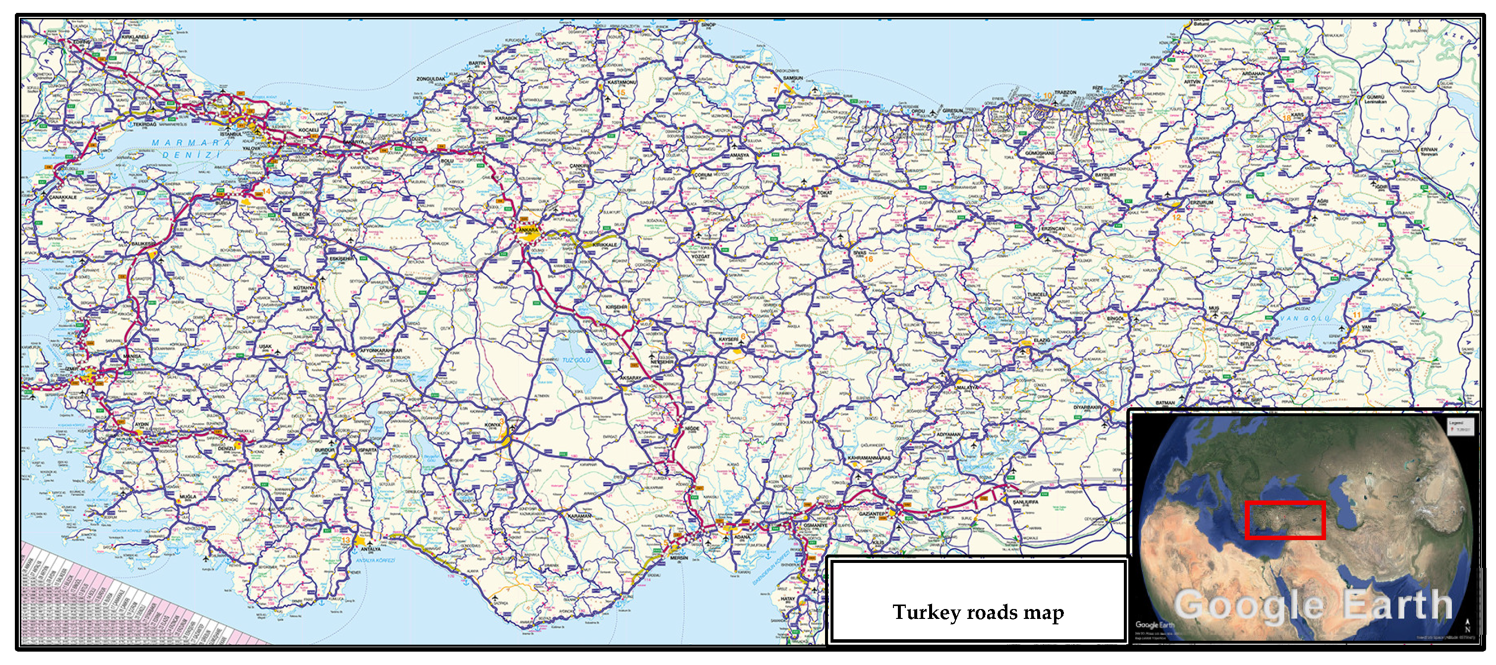
2.1. Study Area

Turkey is located between 36° and 42° north latitude and 26° and 45° east longitude and acts as a bridge between Asia and Europe through the Bosporus and Dardanelles Straits. Due to its geographical position, the country is situated on key trade routes, migration corridors, and major east-west and north-south routes, making it strategically important [25]. The country’s population increased from 56.47 million in 1990 to 84.68 million in 2021. The growth in population substantially influences the escalation in demand for housing, energy, and transportation, particularly in Turkey’s urban regions [26]. According to the 2020 data, Turkey has a road network with a total length of 68,266 km. This network comprises 5% (3095 km) motorways, 45.4% (31,006 km) state roads, and 50.1% (34,165 km) provincial roads [27]. Figure 1 displays a map of state roads in Turkey.

The number of motor vehicle registrations experienced significant growth, rising from 15,095,603 in 2010 to 26,482,847 by 2022. Furthermore, when analyzed by fuel type, the number of petrol cars increased from 3,191,964 to 3,817,104, diesel cars rose from 1,381,631 to 5,261,876, and LPG cars increased from 2,900,034 to 5,005,563 [29]. Despite an annual increase in the overall number of vehicles, car ownership in Turkey remains significantly lower than the European average, primarily because of exorbitant car prices and taxes. Based on the 2019 data, Luxembourg has a car ownership rate of 681 cars per thousand people, Italy has a rate of 663 cars per thousand people, and Turkey has a rate of 150 cars per thousand people. The average for the EU-27 in 2019 was 553 [30].

The Annual Average Daily Traffic (AADT) statistics for every section of Turkey’s state roadways were collected in order to compare the number of cars using these routes between 2010 and 2020. Information regarding the number of vehicles traversing state roads, their classifications, and the distances of the roads was acquired from the reports of the General Directorate of Highways (GDH) spanning 11 years from 2010 to 2020. It was found that the total increased by 60% from 11,193,242 in 2010 to 17,917,138 in 2020 [31]. Although these total values (total AADT numbers) do not clearly show the number of vehicles using the roads, it is significant to notice the rise throughout the years because these increases also increase traffic-related emissions.

2.2. Emission Calculations

An approach commonly used to calculate traffic emissions involves using emission factors [13]. Emission factors are frequently employed to evaluate transport emissions by establishing a correlation between pollutant emissions and vehicle activities and types, such as distance traveled, fuel consumption, and energy consumption [32].

In this study, the number and type of vehicles and the distance traveled on state roads in Turkey, which form the basis of emission calculations, were compiled from the Traffic Transport Information Index published annually by the GDH for the 11 years between 2010 and 2020 [31]. Vehicles were classified as automobiles (Personal Cars—PCs), light commercial vehicles (LCVs), and heavy-duty vehicles (HDVs), and automobiles were classified as petrol, diesel, and LPG according to fuel type [29]. This study classified LCVs and HDVs in Turkey as diesel-fueled vehicles because they mainly use diesel fuel, with some exceptions. Emission factors from the “EMEP/EEA air pollutant emission inventory guide 2023” were utilized in the study. This guide is technical and supports the reporting of emission data under the UNECE Convention on Long-Range Transboundary Air Pollution (CLRTAP) and the EU National Emission Ceilings Directive. In the guide, the tiered approach for emission estimations is divided into three stages, which vary depending on the technological specifics employed in the calculation. In the Tier 1 approach, the calculation is based on the amount of each fuel type and its emission factors (Equation (1)). Compared to other methods, this method allows the collection of the data required for calculations. Tier 2 is similar to Tier 1 in that it uses activity data and emission factors to predict emissions. The primary difference is that this more detailed methodology requires additional information on fuel, technology, and country-specific details. In the Tier 3 methodology, vehicle emissions are calculated primarily based on engine operating conditions (hot-cold) and various driving situations (urban, rural, and highway driving). Factors such as cold starts, seasonal effects, and vehicle idling time can significantly affect emissions under real-world driving conditions. Newer standards (such as Tier 2 and Tier 3) consider these variables more comprehensively, but they were often overlooked under older standards such as Tier 1 [33]. If the data used in these approaches (Tier 2, Tier 3) can be provided, calculations can be more accurate overall. However, it is difficult to obtain data on these approaches for the whole country. Therefore, the calculations were performed using the Tier 1 approach. The calculations employ emission factors from

Table 1. Tier 1 emission factors [34].

Emission	Automobile g/kg			HDV g/kg	LCV g/kg
	Gasoline	Diesel	LPG	Gasoline	Diesel
CO	84.7	3.33	84.7	7.58	7.4
CO2	3.18	3.14	3.017	3.14	3.14
SO2	0.08	0.016	0	0.016	0.016
PM	0.03	1.1	0	0.94	1.52
NOx	8.73	12.96	15.2	33.37	14.91
NMVOCs	10.05	0.7	13.64	1.92	1.54
N2O	0.206	0.087	0.089	0.051	0.056
NH3	1.106	0.065	0.08	0.013	0.038

, and

Table 2. Tier 1 typical fuel consumption per km for each vehicle [34].

Vehicle Category	Fuel	Characteristic Fuel Consumption (g/km)
Automobile	Gasoline	70
	Diesel	60
	LPG	57.5
	E85	86.5
	CNG	62.6
LCV	Gasoline	100
	Diesel	80
HDV	Diesel	240
	CNG	500

displays the fuel consumption data per kilometer for each vehicle category.

$${\mathrm{E}}_{\mathrm{i}}={\sum }_{\mathrm{i},\mathrm{m}}\left({\sum }_{\mathrm{i}}(\mathrm{F}{\mathrm{C}}_{\mathrm{j}}\times \mathrm{E}{\mathrm{F}}_{\mathrm{i},\mathrm{j}}\times \mathrm{V}\mathrm{R}\mathrm{L})\right)$$

(1)

where E_i is the daily amount of emissions (g/km), FC_j is the fuel consumption (g-fuel/km), EF_i,j is the emission factor (g/kg fuel), VRL is the vehicle road length (km), i is the type of pollutant, j is the fuel type, and m represents the total values for all.

Data on the distribution of registered cars based on fuel type were sourced from TurkStat for 11 years. Using these rates in the calculations, the distribution of cars based on fuel type was calculated. The corresponding graph is shown in Figure 2.

2.3. Future Predictions

In this study, polynomial regression was employed to model the nonlinear growth trend in the number of registered vehicles in Turkey. The accuracy of predicting future vehicle counts using the polynomial regression method is contingent on the breadth of the past information set. Moreover, more information is needed to estimate the number of vehicles traveling on state roads in the study area, which is used for emission calculations. Therefore, TurkStat’s data on the number of vehicles registered for traffic in Turkey from 1966 to 2021 were used in the estimation study.

A second-degree polynomial model was selected for its ability to capture the long-term curvature in the data without introducing excessive model complexity. The model was implemented using Python 3.7 (Python Software Foundation, Beaverton, Oregon, ABD) and the scikit-learn 1.4.2 library (Machine learning in Python Version 1.4.2). The model pipeline included PolynomialFeatures and LinearRegression, and the regression coefficients were estimated using the least squares method. The model achieved a coefficient of determination (R²) of 0.96, indicating a strong fit between the observed and predicted values. Additional performance metrics such as Root Mean Square Error (RMSE) and Mean Absolute Error (MAE) and the high R² value indicate that the model provides sufficient accuracy for projection purposes. To minimize the risk of overfitting, higher-degree polynomial models were not considered, as they tend to increase model variance and reduce generalizability.

The number of automobiles from 1966 to 2021 was analyzed to project the trend for the years up to 2050. This projection enabled the calculation of future emissions based on average per-vehicle emissions and emission factors defined in the EMEP/EEA air pollutant emissions inventory guide. For future emission predictions, GHG emissions were calculated based on the number of vehicles using state roads, and the average emissions per vehicle (Equation (2)) were calculated considering the total number of vehicles. Then, emissions were estimated using average emission amounts per vehicle and the number of vehicles projected for the future.

$$MVE={\displaystyle \frac{{\sum }_{t=n}^p {Em}_t}{{\sum }_{t=n}^p {Veh}_t}}$$

(2)

where MVE is the mean vehicle emissions (kg emission/per vehicle), n is the first year used in the calculation, p is the final year used in the calculation, Em is the calculated emission value (kg), and Veh is the number of vehicles.

This method provides a solid framework for forecasting future emissions and analyzing long-term trends. Using this and comparable predictive models may be valuable for forecasting.

In the study, the Relative Standard Error (RSE) values were calculated to determine the uncertainty (Equation (3)). The Relative Standard Error (RSE) offers a dimensionless, percentage-based indicator of the uncertainty, thereby allowing for better comparability across datasets or studies.

$$RSE={\displaystyle \frac{SE}{\overline{x}}}\times 100$$

(3)

where SE represents the Standard Error, and $\overline{x}$ is the arithmetic mean of the data [35].

The Standard Error (SE) quantifies the uncertainty in how accurately a sample mean estimates the population mean. A smaller SE indicates greater reliability of the estimate and is calculated according to Equation (4) [36,37].

$$SE={\displaystyle \frac{\sigma }{\sqrt{n}}}$$

(4)

where σ is the standard deviation, and n refers to the sample size

According to the Australian Bureau of Statistics (ABS), RSE values between 0–25% are considered reliable and suitable for publication and interpretation. RSEs between 25–50% indicate a high sampling error and should be interpreted with caution, while RSEs exceeding 50% reflect excessive uncertainty, rendering the estimates unreliable and unsuitable for publication [38].

2.4. Polynomial Regression

Regression is a crucial topic in data mining that is used to predict a specific outcome by considering relevant input factors. The data-driven model is unsuitable for linear prediction in some engineering computations. When faced with such situations, employing a suitable curve for the given data is advisable. Polynomial regression is a widely used method for data analysis [39,40]. It offers an advantage over linear models by providing high flexibility in modeling nonlinear data relationships. Thanks to its flexible structure, it can capture complex trends and shapes. Therefore, the model can fit the data better [41]. This method offers high accuracy in capturing nonlinear relationships and fitting curves, enabling the representation of more complex data relationships [42]. Polynomial regression using too much data may cause overfitting. In this case, the model may perfectly predict the data it was trained on but may fall short on new data. Additionally, outliers can seriously degrade the accuracy of the model. It is also important to determine the appropriate polynomial degree; lower degrees may be insufficient, while higher degrees may create unnecessary complexity. Therefore, these factors should be carefully considered when creating a model [42,43].

Polynomial regression, involving a single independent variable denoted as X, is a specific instance of multiple regression. The formula below represents the univariate polynomial regression model. K represents the degree of the polynomial. The degree of the polynomial is a parameter that quantifies the model’s intricacy level. Effectively, this is equivalent to having a multi-model with the variables X₁ = X, X₂ = X², and X₃ = X³, and its formula is expressed in Equation (5) [44].

y_i = β₀ + β₁x_i + β₂x_i ² + β₃x_i ³ … +β_kx_i ^k + ε_i, for i = 1,2, …, n

(5)

where y is the dependent variable, x is the independent variable, k is the polynomial degree, β₀, β₁, …, β_k are constant coefficients, and ε_i is the error between the model and the observations.

The coefficient of uncertainty is calculated using Equation (6), where R² is the coefficient of uncertainty. This value is used to show the relationship between variables. The variable takes a value between 0 and 1 when calculated using the foregoing formula. The nearness of R² to 1 indicates good agreement between the values.

$$R^2={\displaystyle \frac{S_t-S_r}{S_t}}$$

(6)

where S_t is the total sum of squares, and S_r is the residual sum of squares [45].

In this study, a quadratic polynomial regression model was developed to analyze historical trends and predict the future number of motor vehicles in Turkey. The dataset (1966–2021) was processed using Python and split into training (80%) and testing (20%) subsets. Model performance was evaluated using standard error metrics, particularly RMSE and MAE. RMSE, which penalizes larger errors more heavily, is suitable in contexts where large deviations are critical, whereas MAE provides a straightforward interpretation of the average prediction error in actual units (Equations (7) and (8)) [46].

$$RMSE=\sqrt{{\displaystyle \frac{1}{n}}{\sum }_{i=1}^n( y_i-{\widehat{y}}_i{)}^2}$$

(7)

$$MAE={\displaystyle \frac{1}{n}}{\sum }_{i=1}^n\left|y_i-{\widehat{y}}_i\right|$$

(8)

where $y_i$ is the true value, ${\widehat{y}}_i$ is the predicted value, n is the total number of observations.

2.5. Distribution Maps

During the development of spatial distribution maps, a shapefile (.shp) containing the administrative boundaries of Turkey’s 81 provinces was utilized as the base layer. The coordinate reference system was defined as WGS 84 (World Geodetic System 1984) within the QGIS (Quantum GIS- QGIS Development Team-Version 3.10) environment. Attribute data comprising the calculated pollutant emission values for the years 2010 and 2020 was manually entered into the GIS attribute table. The spatial distribution of emissions was then visualized using the “Graduated” symbology option in QGIS, applying the “Equal Interval” classification method to represent emission intensity across provinces.

3. Results

3.1. Greenhouse Gas Emission Calculations from State Roads

This study examined the emissions of direct GHGs, primarily CO₂ and N₂O, and indirect GHGs, including NH₃, NO_X, SO₂, CO, NMVOC, and PM, all of which contribute to the indirect greenhouse effect. The calculations were performed for 11 years, from 2010 to 2020. The results obtained are given in

Table 3. The levels of CO₂, N₂O, NH₃, NO_X, SO₂, CO, NMVOC, and PM emissions (kg/day) from road traffic between 2010 and 2020.

		2010	2011	2012	2013	2014	2015	2016	2017	2018	2019	2020	Total	σ	RSE %	Increase %
CO2	PC	20,074	21,499	22,444	23,066	25,735	28,765	29,559	32,605	33,073	33,677	31,075	301,572	5033.02	5.54	54.8
	LCV	2595	2757	2755	2639	2716	2824	2866	4211	5176	5192	4870	38,601	1104.28	9.49	87.6
	HDV	29,125	31,778	32,255	33,508	34,346	36,095	35,949	36,263	32,342	31,440	31,202	364,303	2323.82	2.12	7.1
	Total	51,794	56,034	57,454	59,213	62,797	67,684	68,374	73,079	70,591	70,309	67,147	704,476	6985.10	3.29	29.6
N2O	PC	927	952	962	963	1052	1159	1180	1288	1293	1306	1208	12,289	150.08	45.50	30.3
	LCV	46	49	49	47	48	50	51	75	92	92	86	687	19.56	45.78	85.9
	HDV	473	516	524	544	558	586	584	589	525	506	502	5907	38.52	45.47	6.1
	Total	1446	1517	1535	1554	1658	1795	1815	1952	1911	1903	1796	18,883	180.55	45.48	24.2
NH3	PC	3621	3512	3384	3248	3427	3684	3692	3894	3897	3878	3604	39,840	216.99	1.81	-0.4
	LCV	31	33	33	32	33	34	35	51	63	62	58	466	13.24	9.45	85.9
	HDV	121	132	134	139	142	149	149	150	134	129	128	1506	9.64	2.12	6.1
	Total	3773	3676	3551	3419	3602	3867	3876	4095	4094	4069	3791	41,812	227.73	1.81	0.5
NOX	PC	75,685	82,983	88,058	91,549	102,979	115,481	118,783	131,273	133,557	136,143	125,361	1,201,852	21,924.09	6.05	65.6
	LCV	12,323	13,093	13,081	12,529	12,896	13,412	13,608	19,996	24,578	24,419	22,904	182,840	5181.09	9.40	85.9
	HDV	309,519	337,716	342,788	356,105	365,007	383,594	382,044	385,381	343,707	330,964	328,461	3,865,286	25,211.01	2.16	6.1
	Total	397,527	433,792	443,927	460,183	480,883	512,486	514,435	536,650	501,842	491,526	476,726	5,249,977	40,768.56	2.58	19.9
PM	PC	1333	1669	1948	2212	2672	3229	3518	4080	4306	4535	4212	33,714	1155.74	11.37	216.0
	LCV	1256	1335	1334	1277	1315	1367	1387	2038	2506	2489	2335	18,640	528.17	9.40	85.9
	HDV	8719	9513	9656	10,031	10,282	10,805	10,762	10,856	9682	9323	9252	108,881	710.17	2.16	6.1
	Total	11,308	12,517	12,938	13,520	14,269	15,402	15,668	16,975	16,493	16,347	15,799	161,235	1862.13	3.83	39.7
SO2	PC	262	255	248	240	256	279	282	306	303	304	283	3018	23.65	2.60	8.3
	LCV	13	14	14	13	14	14	15	21	26	26	25	196	5.55	9.44	85.9
	HDV	148	162	164	171	175	184	183	185	165	159	157	1853	12.20	2.18	6.1
	Total	423	431	426	424	445	477	480	512	494	489	465	5068	32.09	2.10	9.9
CO	PC	453,721	468,080	473,381	470,859	509,985	551,676	551,665	593,340	589,312	588,222	540,609	5,790,849	53,468.35	3.06	19.2
	LCV	6116	6498	6492	6218	6401	6656	6754	9924	12,199	12,120	11,367	90,746	2571.58	9.40	85.9
	HDV	70,307	76,712	77,864	80,889	82,911	87,133	86,781	87,539	78,073	75,178	74,610	878,000	5726.63	2.16	6.1
	Total	530,144	551,290	557,737	557,966	599,297	645,466	645,200	690,803	679,584	675,520	626,587	6,759,595	57,956.62	2.84	18.2
NMVOC	PC	62,327	65,186	66,602	66,754	72,717	78,861	78,929	85,036	84,670	84,638	77,661	823,380	8514.47	3.43	24.6
	LCV	1273	1352	1351	1294	1332	1385	1406	2065	2539	2522	2366	18,885	535.20	9.40	85.9
	HDV	17,809	19,431	19,723	20,489	21,001	22,071	21,982	22,174	19,776	19,043	18,899	222,396	1450.56	2.16	6.1
	Total	81,408	85,969	87,676	88,537	95,050	102,317	102,316	109,275	106,984	106,203	98,925	1,064,660	9601.79	2.99	21.5

.

When the results of the study were evaluated (Table 3), the amounts of CO₂, N₂O, NH₃, NO_X, SO₂, CO, NMVOC, and PM increased by 29.6%, 24.2%, 0.5%, 19.9%, 9.9%, 18.2%, 21.5%, and 39.7%, respectively, in 11 years. Of all the contaminants, the PM showed the highest increase of 39.7%, while the NH₃ showed the smallest increase of 0.5%. This situation relates to the types of fuel used by vehicles. An analysis of the fuel types of vehicles used in traffic reveals that diesel cars, LPG-fueled cars, LCVs, and HDVs have experienced growth rates of 3.60, 1.64, 2.06, and 1.15 times, respectively, over the past 11 years. In contrast, petrol cars have seen a decline of 0.82%. Diesel-fueled automobiles, LCVs, and HDVs collectively account for almost 50% of all vehicles on the road. Although diesel-powered cars produce more PM emissions than petrol-powered vehicles, petrol-powered vehicles emit more NH₃ emissions than diesel-powered vehicles [34]. Consequently, while the type and quantity of emissions vary depending on the fuel used, the dominance of oil as the primary fuel in the transportation sector is highly significant. A review of the literature reveals that the increases in traffic-related greenhouse gas emissions in Turkey and other nations are noteworthy [20,24,47,48]. To mitigate the rise in GHG emissions, one practical approach is to impose restrictions on the use of fossil fuels. To achieve carbon neutrality across all sectors, including transportation, the European Union has declared its intention to prohibit the sale of diesel and petrol automobiles entirely by 2035 [49]. Nevertheless, the rate at which the automobile sector in Turkey is adapting to this transition is unclear. Anticipating its global ubiquity is an inaccurate perspective. Fluctuations and advances in the transportation industry are varied. It is recommended to use numerous preventive applications to provide higher precision in reaching the desired effect.

Upon analyzing the calculated emission values, a consistent rise became evident between 2010 and 2018 (Table 3). However, between 2018 and 2020, the levels of CO₂, N₂O, NH₃, NO_X, SO₂, CO, NMVOC, and PM decreased by 3.9%, 6.4%, 8%, 5.3%, 6.3%, 8.5%, 8.1%, and 4.4%, respectively. The decrease in the number of cars on the roadways covered in the research may be attributed to the impact of lockdown, which reduced vehicle traffic during the pandemic. Specifically, vehicles decreased from 19,379,148 in 2018 to 19,132,034 in 2019 and 17,917,138 in 2020. Schools, colleges, shops, restaurants, and gyms, where people congregate in large groups, were temporarily shut down due to restrictions. In addition to solutions to reduce the number of trips on public transportation, isolation measures were also implemented among the population. As a result of these measures, access to shops and transportation hubs was reduced by around 80%, and access to workplaces was decreased by about 45% [50,51]. These applications indicate the cause of the decrease in car usage. Furthermore, the construction of highways, tunnels, and bridges to enhance the efficiency, cost-effectiveness, sustainability, and environmental friendliness of road transportation nationwide may also have a positive impact. The road network, which was 62,864 km in the early 2000s, has risen to 68,266 km in the 2020s, and the number of tunnels has increased from 83 to 488 [27]. Therefore, part of the reduction in emissions in these years can also be attributed to a decrease in the distances traveled.

Emission estimates were assessed for statistical reliability using RSE values. CO₂, NH₃, NO_X, PM, SO₂, CO, and NMVOC emissions showed low uncertainty, with RSE values generally below 10%, indicating high reliability. CO₂ estimates, in particular, had RSEs of 5.54% (PC), 9.49% (LCV), and 2.12% (HDV), with a total value of 3.29%. In contrast, N₂O emissions exhibited high uncertainty across all categories, with RSEs of around 45%. Overall, the results confirm that most emission estimates are statistically robust, except for N₂O.

Figure 3 displays the distribution of overall CO₂, N₂O, NH₃, NO_X, SO₂, CO, NMVOC, and PM emissions between 2010 and 2020, originating from vehicles that were in transit on the roadways included in the research, categorized by vehicle type. Automobiles account for 58% of all emissions. When assessing pollutant sources, PCs are shown to be responsible for 65% of N₂O, 95% of NH₃, 59% of SO₂, 86% of CO, and 77% of NMVOC pollutants. In contrast, HDVs accounted for 52% of CO₂, 74% of NO_X, and 67% of PM pollutants. One kilogram of gasoline in a car emits 3.18 g of CO₂, while one kilogram of diesel fuel emits 3.14 g [34]. Compared to gasoline-powered vehicles, diesel vehicles release fewer CO₂ emissions. However, HDVs are accountable for 52% of CO₂ since diesel fuel use, in contrast to gasoline, has been on the rise over time. Given that diesel fuel is used as the primary source of energy in HDVs, it would be advantageous to implement enhancements focused on fuel to mitigate emissions of CO₂, NO_X, and PM.

To analyze the spread of emissions from automobiles on state highways in Turkey, emission distribution maps for 2010 and 2020 were generated using QGIS. The resulting maps are shown in Figure 4. The charts clearly illustrate that the emission levels in 2010 were more significant in western and central Anatolia. Furthermore, it is evident that emissions continued to increase until 2020. The results are summarized by the item below:

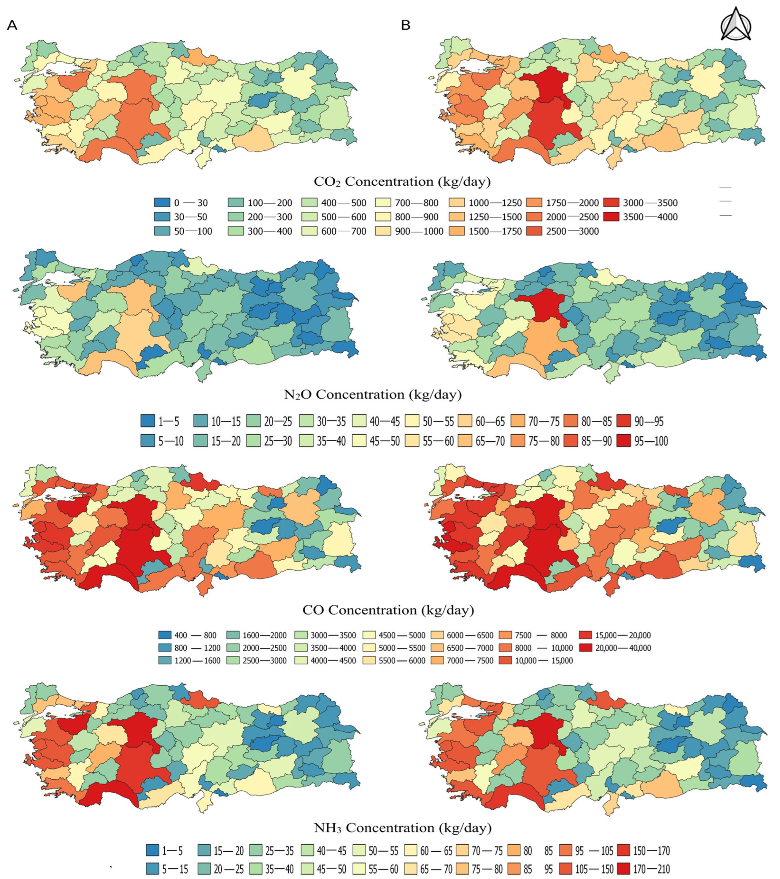
• The daily CO₂ ranged from 47.8 to 2429 kg in 2010 and increased from 98.74 to 3024.8 kg in 2020. In 2010, Konya province had the highest recorded CO₂ emissions. In contrast, Ankara province had the highest values reported in 2020.
• The daily N₂O in 2010 ranged from 1.21 to 69.53 kg/day, whereas in 2020, it ranged from 1.72 to 97.94 kg/day. Emissions were significantly elevated, particularly in central Turkey. In 2010, the province with the highest emissions was Bursa. In 2020, it was Antalya.
• The daily CO ranged from 406.06 to 26,895.91 kg/day in 2010 and from 599.12 to 34,543.22 kg/day in 2020. In 2010, Antalya province had the highest recorded emission amount. In 2020, it was Ankara.
• NH₃ was calculated in the range of 2.75–196.82 kg/day in 2010 and 3.63–209.54 kg/day in 2020. The highest emission quantity was calculated in Antalya in 2010 and in Ankara in 2020.
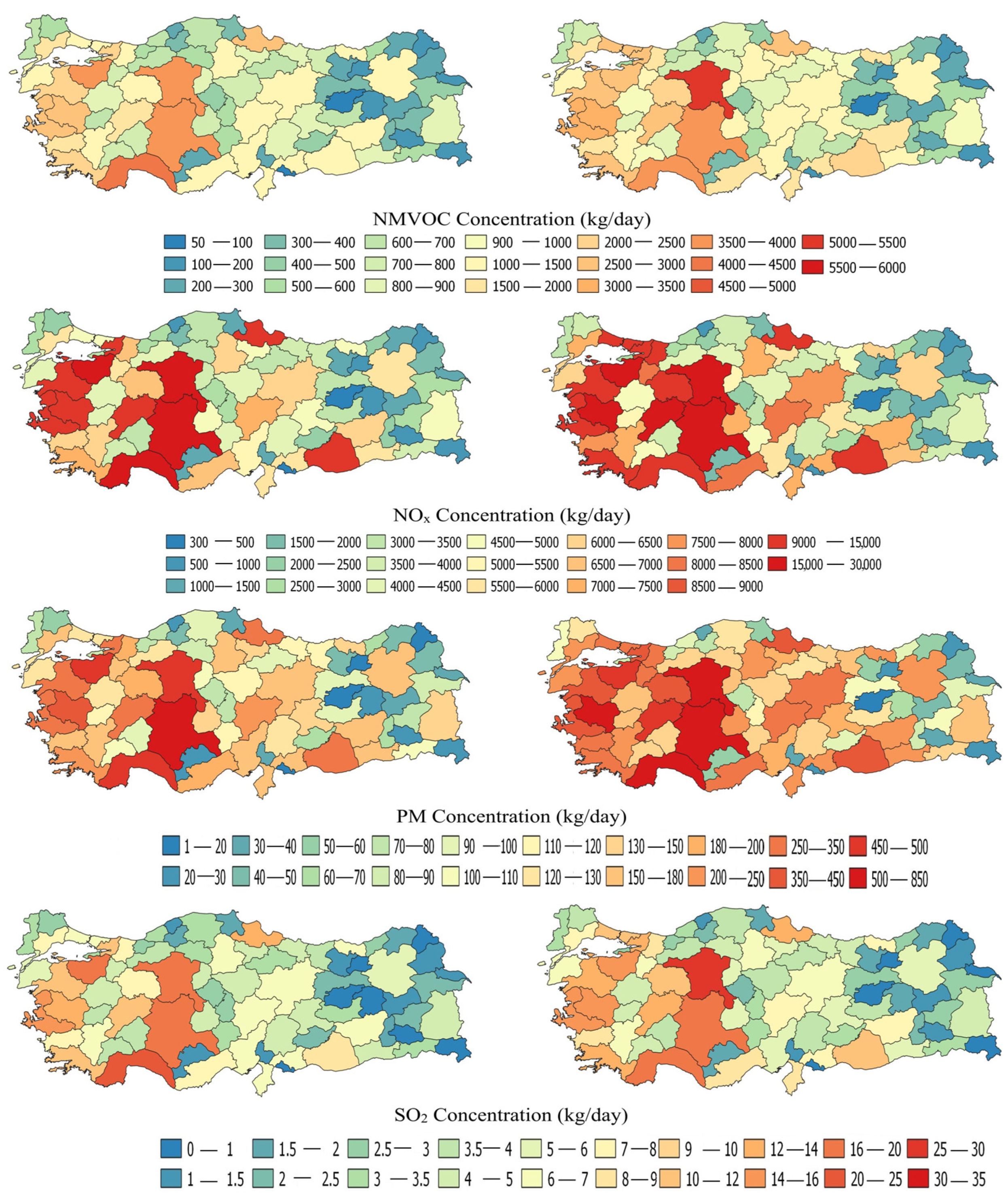
• When NMVOC levels were examined, the values ranged between 64.83 and 4030.7 kg/day in 2010. Antalya has the highest calculated emissions. In 2020, there was a change between 94.42 and 5436.84 kg/day, and the highest emission was calculated in Ankara.
• NO_X amounts were calculated as 330.67–19,470.02 kg/day and 446.55–25,733.49 kg/day for 2010 and 2020, respectively. The calculated maximum emissions were for Konya and Ankara, respectively.
• The daily quantity of PM10 was calculated to be 9.20–551.12 kg in 2010 and 15.51–835.51 kg in 2020. The provinces of Konya and Ankara had the highest emission quantities for 2010 and 2020, respectively.
• In Turkey, the amount of SO₂ emissions was calculated to be 0.35–20.19 kg/day in 2010 and 0.44–25.30 kg/day in 2020. Antalya (in 2010) and Ankara (in 2020) were determined to have the maximum emission quantities.

Based on the calculations, while there are variations in emissions levels throughout the provinces, the cities of Ankara, Antalya, and Bursa consistently exhibit the highest rises in emissions. This might be attributed to the rise in population and subsequent increase in vehicular traffic in these cities. Between 2010 and 2022, the population of Ankara increased from 4,771,716 to 5,782,285, the population of Antalya climbed from 1,978,333 to 2,688,004, and the population of Bursa increased from 2,605,495 to 3,194,720 [26].

Rapid population expansion leads to rapid urbanization. During the evaluation of provinces for the year 2020, Istanbul, with a population density of 2427 people per square kilometer, Kocaeli, with a population density of 454 people per square kilometer, and Izmir, with a population density of 324 people per square kilometer, ranked as the top three provinces in terms of population density. Tunceli has a population density of 10 people per square kilometer, which is the lowest among these provinces. The provinces of Bursa, Ankara, and Antalya, which see the highest increases in emissions, are rated 7th (241 individuals per square kilometer), 9th (186 individuals per square kilometer), and 23rd (97 individuals per square kilometer). Kocaeli province ranks highest in GHG emissions per square kilometer, with values of 5056 g/km² for CO, 475 g/km² for CO₂, 14 g/km² for N₂O, 32 g/km² for NH₃, 3 g/km² for SO₂, and 778 g/km² for NMVOC. Yalova province ranks first in NO_X emissions (3365 g/km²) and PM emissions (112 g/km²). Bilecik has the highest per capita GHG emissions for CO, CO₂, N₂O, NH₃, NO_X, PM, SO₂, and NMVOC, with values of 31, 4, 0.1, 0.2, 37, 1, 0.03, and 5 g/person, respectively. These provinces are characterized by a high degree of urbanization. Urbanization results in environmental degradation, pollution, physical disorganization, and anomalies in settlement. Sustainability plays a crucial role in the growth and development of cities. To achieve the environmental goals of sustainability, urban design should include the characteristics of the local climate, ecosystems, energy, water, and resource flows. This planning approach aims to incorporate communities into the natural environment, decrease reliance on vehicles, optimize resource utilization, and showcase the area’s unique characteristics [52].

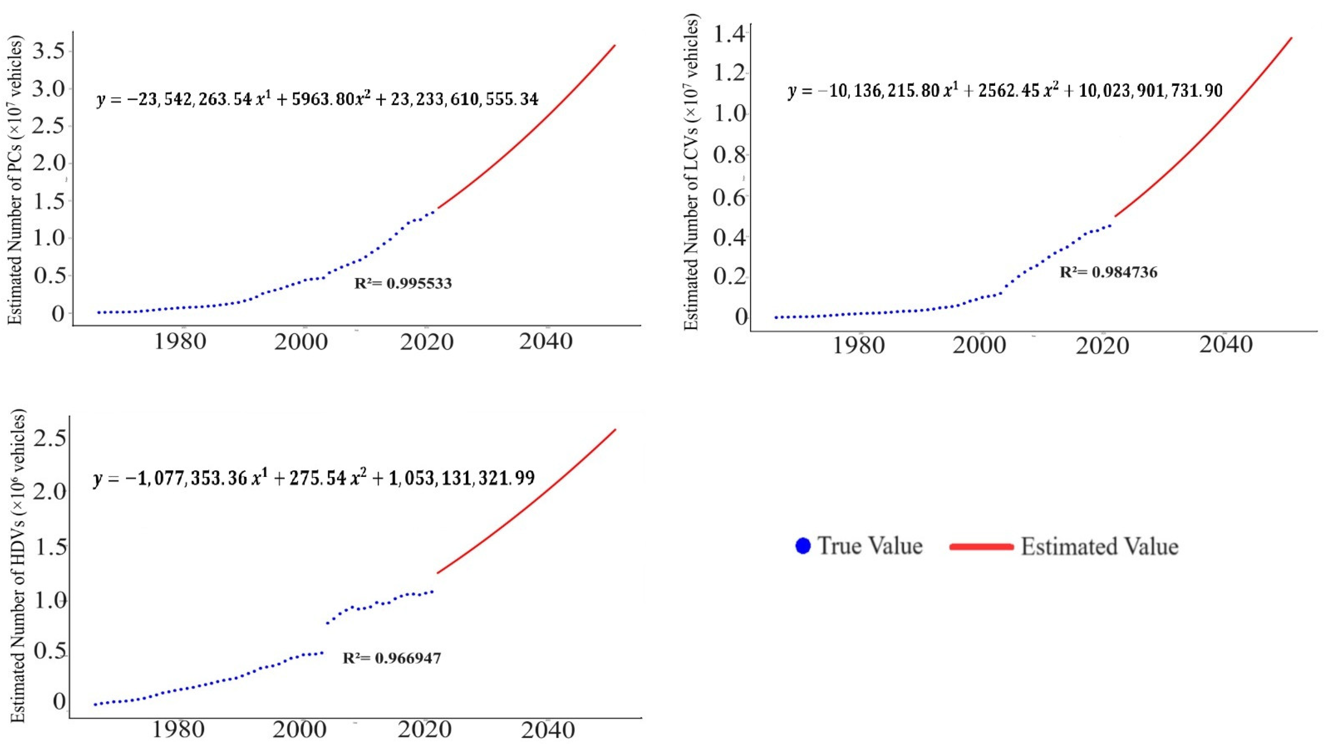
3.2. Emission Estimates for Future Years

This study used the polynomial regression approach to predict the number of vehicles up to the year 2050. The findings of this analysis are presented in Figure 5. The following equations were used to predict future outcomes:

PC : y = −23542263.54 x¹ + 5963.80 x² + 23233610555.34 (R² = 0.996)

(9)

LCV : y = −10136215.80 x¹ + 2562.45 x² + 10023901731.90 (R² = 0.985)

(10)

HDV : y = −1077353.36 x¹ + 275.54 x² + 1053131321.99 (R² = 0.967)

(11)

where y is the dependent variable (number of vehicles in the future), and x is the independent variable (number of vehicles in the past).

The registered vehicle count, which stood at 26,482,847 in 2022, is projected to have grown by 105%, reaching 50,701,935 by 2050. The projected figures indicate that there will be 34,855,102 PCs, 13,344,351 LCVs, and 2,502,482 HDVs.

There are different methods for estimation in the literature. Irhami and Farizal estimated the number of vehicles in Indonesia using the ARIMA (Auto Regressive Integrated Moving Average) method. The estimate for the next 11 years was based on historical data from 2001 to 2019. As a result of the research, the best estimation models were determined as ARIMA for cars and ARIMA for motorcycles. The article explains that the increasing number of automobiles generates various difficulties, including traffic congestion, air pollution, and traffic accidents, and emphasizes the need to predict future vehicle numbers to mitigate such problems [53]. Sekula et al. used machine learning (ML) and vehicle measurement data to estimate historical hourly traffic levels on Maryland’s road network. The study was aimed at improving the correct prediction of hourly traffic volumes in areas with few sensors. In addition to the current profiling approach, a model was created using an artificial neural network (ANN). This technology produces 24% more accurate volume estimations than the profiling method utilized throughout the United States [54]. Sayed et al. conducted a comprehensive evaluation of machine learning (AI)-based approaches for traffic flow prediction. The study focuses on Intelligent Transportation Systems (ITSs) and the impact of machine learning (ML) and deep learning (DL) techniques used in these systems on traffic prediction. The difficulties observed in implementing these techniques were discussed in the paper [55]. Alhindawi et al. estimated greenhouse gas (GHG) emissions from the road transportation sector in North America using multivariate regression and double exponential smoothing (DES) models. The purpose of the research was to contribute to the development of strategic decisions to minimize GHG emissions by calculating existing and future emissions. The results revealed that kilometers traveled and the number of vehicles have a substantial impact on greenhouse gas emissions [56].

According to studies, the number of vehicles on the road is going to rise steadily. This means a rise in emissions. Turkey implemented the EURO 5 standards in October 2009 and the EURO 6 standards in January 2015 with the aim of decreasing pollution levels in newly manufactured vehicles. In 2021, an analysis of registered vehicles by age group revealed that 23.1% fall within the 0–15 years range, 24.6% fall within the 6–110 years range, 15.8% fall within the 11–15 years range, 10.2% fall within the 16–120 years range, and 26.3% are older than 21 years [57]. Hence, while these norms will partially regulate the pace of emission growth, more is needed. Therefore, emissions predictions were also made based on the estimated number of vehicles up to 2050. The graphs are shown in Figure 6. Upon analyzing Figure 6, it becomes evident that each emission type has a consistent upward tendency as time passes. The ratios for CO₂, N₂O, NH₃, NO_X, PM10, SO₂, CO, and NMVOC are 149.17%, 151.78%, 154.39%, 138.95%, 151.47%, 150.97%, 153.09%, and 152.09%, respectively. External factors, such as future technological developments, changes in economic conditions, or policy interventions that could significantly affect future vehicle use and emissions, may suggest that increases in emissions will not occur at this rate. However, there were also developments between 2010 and 2020, and despite these developments, an increase in emissions was observed. The effectiveness of existing emission reduction policies between these years was insufficient. From this perspective, it is thought that the results of the study reflect the developments in the transportation sector and environmental policy, and that there will be emission increases at these rates in the future under current conditions. Due to the rise in GHG emissions, there is a growing concern about global climate change. This poses a potential danger to the ecosystem and living organisms, leading to extreme conditions such as changes in precipitation, humidity, air movement, and temperature. Therefore, it is necessary to implement stricter environmental regulations, penalties, and policies to shift towards alternative transportation modes, or urban planning changes that could alter vehicle usage patterns to address this issue. There are studies in the literature that produce recommendations for reducing greenhouse gas emissions. For example, Doğan Güzel and Alp conducted a study to analyze the effects of the transport sector on climate change in Istanbul, the most populous city in Turkey, which has a high vehicle density. They used a model to estimate GHG emissions from 2016 to 2050. They employed the Integrated Markal-EFOM System (TIMES), a technologically advanced and cost-effective model to achieve this objective. In addition, they examined three different possibilities concerning electric rail transportation (Scenario 1), electric and hybrid vehicles (Scenario 2), and restricted CO₂ emissions (Scenario 3). The findings indicated that by 2050, Scenario 1 would result in a 1.1% decrease in GHG emissions, Scenario 2 would lead to an 11% reduction, and Scenario 3 would achieve a significant 39% decrease [18].

The literature discusses seven primary themes for achieving sustainable transportation by mitigating GHG emissions. Strategies to achieve these goals include the use of alternative fuels, the promotion of fuel-efficient vehicles, decreasing vehicle use, reducing transportation infrastructure, the implementation of intelligent transport systems, the integration of various modes of transportation, and reducing overall travel [58]. These issues primarily encompass strategies aimed at mitigating or, at the very least, limiting the release of GHG emissions throughout the lifespan. GHG emissions are also generated during the manufacturing and application phases. To effectively minimize GHG emissions, it is important to consider further options for raw material supply/production, mixture/road design, and casting/compaction procedures at this stage. GHG emissions from road building in China have been evaluated using the life cycle assessment approach at both the national and provincial levels, and these calculations have been performed independently from the use of fossil fuels. Chen et al. highlighted the need for increased focus on GHG emissions associated with road construction. The study also investigated the impact of various factors on GHG emissions, such as the construction of concrete and asphalt roads, road classification, number of lanes, and road length. It also highlighted the presence of GHG emissions during the pre-service period of the road, which included the application phase starting from raw material production [59]. These studies demonstrate the importance of addressing the whole issue comprehensively and considering all its dimensions.

The polynomial regression model yielded an RMSE of 310,527 and an MAE of 260,123 for predicting PC registrations over the 2019–2021 period. These results indicate that the model deviates from actual values by approximately 260,000 vehicles on average, with RMSE reflecting the influence of higher-magnitude errors on overall model performance. The LCV prediction model yielded an RMSE of 211,415 and an MAE of 189,297, indicating an average deviation of approximately 189,000 vehicles from actual values. While the model captures historical trends with reasonable accuracy, year-to-year fluctuations may limit its precision at finer temporal scales. The HDV prediction model produced an RMSE of 57,221 and an MAE of 41,770, indicating an average deviation of approximately 42,000 vehicles. The relatively low error values suggest strong predictive accuracy and a close alignment with historical HDV registration trends. It should be noted that polynomial regression models assume trend continuity and may fail to capture disruptive changes in technology, policy, or behavior, which can substantially alter future emission trajectories.

Turkey needs to immediately implement several measures to achieve its goal stated at the 27th Conference of the Parties (COP 27) in addressing climate change. Although sophisticated technology and low emissions are essential, it is important to acknowledge that our nation’s sluggish pace of vehicle replacement may delay the noticeable effects of new technology vehicles on overall emissions. To meet the desired objectives, it may be imperative to enforce financial measures and incentives to encourage the removal of vehicles manufactured with outdated technology from the current traffic fleet. This may promote a transition toward more efficient motor vehicles. Furthermore, increasing the number of absorption zones can reduce the country’s emissions by capturing and storing them. Based on Ministry statistics, approximately 9% of the country’s CO₂ equivalent emissions were effectively captured and decreased in wooded regions, spanning around 23 million hectares in 2020. The sequestration patterns in 2020 exhibited a 3% rise compared with the data from 1990 [57,60]. It may be advantageous to further increase this growth rate.

4. Conclusions

The present study revealed a significant and rapid increase in vehicle numbers on Turkey’s roads between 2010 and 2020. Although growing alternative transportation networks have yielded benefits, the increased number of vehicles in the transportation sector has led to a rise in fossil fuel use and, consequently, greenhouse gas emissions. Unless the proportion of fossil fuels in the global energy mix declines, these emissions will continue to rise.

Automobiles are responsible for about half of all vehicle-related pollutants. However, diesel fuel used in HDVs is accountable for a considerable part of CO₂ emissions, a significant greenhouse gas. This situation demonstrates the need for improvements in the use of diesel fuel.

When the calculated emission quantities by province were studied, Ankara, Antalya, and Bursa were determined to be the three cities with the highest emissions, despite several variances. The Kocaeli and Yalova provinces were rated as having the highest GHG emissions per square kilometer, whereas the Bilecik province was determined to have the most significant GHG emissions per person. The increase in emissions was a result of urbanization and the increasing number of vehicles. Therefore, governments are advised to develop strategies to reduce emissions from transportation, particularly targeting large cities.

According to the future forecast study, a 105% rise in the number of registered automobiles is projected by 2050. This logically implies that if the advances, initiatives, and policies enacted between 2010 and 2020 continue in the same manner, and no measures are taken, emissions will rise by more than 100%.

It is essential to highlight that energy consumption contributes to the rise in specific GHG emissions, specifically CO₂. To keep GHG emissions as low as possible, reduce pollutant emissions, and meet the 2053 net zero target, it is critical to develop transportation transformation targets that are aligned with global emission reduction strategies, ensure a shift to more sustainable railway/maritime transportation, increase efficiency and clean energy use in transportation strategies, and keep up with new technological developments. Furthermore, higher environmental standards and regulations must be implemented to lessen the link between transportation frequency and greenhouse gas emissions.

For future research, it is recommended to develop scenarios that explore how different numbers of vehicles and fuel types on roadways might reduce greenhouse gas emissions in the transportation sector. Incorporating spatial regression techniques, such as Geographically Weighted Regression (GWR), can effectively address spatial autocorrelation in emission models, thereby enhancing the interpretability and accuracy of GIS-based analyses.

Limitations of the study: This study is limited to state roads, which constitute only 45.4% of the total roads. Provincial roads comprise 50.1% of the total. Nevertheless, they were excluded since there are no vehicle statistics for these roads. Similarly, motorways, which account for 5% of the total, were excluded because of their low proportion. However, the motorways are very heavily used, so when considering the emissions generated by traffic on these motorways, it would be reasonable to say that the amount of emissions from all types of road transportation in Turkey is higher than those calculated in this study. There are three approaches (tiers) for emission estimations. The Tier 2 and Tier 3 approaches provide more accurate results because they require more detailed information than Tier 1. However, it is difficult to obtain detailed data for the entire country. Therefore, calculations were performed using the Tier 1 approach in this study. This situation is seen as a study limitation, even though it is acceptable for macro-level analysis.

References

1. EEA. European Environment Agency. About Climate Change. 2016. Copenhagen, Denmark. Available online: https://www.eea.europa.eu/tr/themes/climate/about-climate-change (accessed on 31 January 2019).
2. IPCC Fourth Assessment Report: Climate Change 2007: Working Group I: The Physical Science Basis. Geneva, Switzerland. Available online: https://archive.ipcc.ch/publications_and_data/ar4/wg1/en/spmsspm-direct-observations.html (accessed on 3 June 2025).
3. Jaroszweski, D.; Chapman, L.; Petts, J. Assessing the potential impact of climate change on transportation: The need for an interdisciplinary approach. J. Transp. Geogr. 2010, 18, 331–335. [Google Scholar] [CrossRef]
4. Carlsson Kanyama, A.; Carlsson Kanyama, K.; Wester, M.; Snickare, L.; Söderberg, I.L. Climate change mitigation efforts among transportation and manufacturing companies: The current state of efforts in Sweden according to available documentation. J. Clean. Prod. 2018, 196, 588–593. [Google Scholar] [CrossRef]
5. IPCC Climate Change 2021 The Physical Science Basis, Working Group I Contribution to the Sixth Assessment Report of the Intergovernmental Panel on Climate Change. Geneva, Switzerland. Available online: https://www.ipcc.ch/report/ar6/wg1/downloads/report/IPCC_AR6_WGI_FullReport.pdf (accessed on 3 June 2025).
6. DCC, Directorate of Climate Change, Repuclic of Turkey Ministry of Environment, Urbanization and Climate Change. Republic of Türkiye Updated First Nationally Determined Contribution. 2024. Ankara, Turkey. Available online: https://unfccc.int/sites/default/files/NDC/2023-04/T%C3%9CRK%C4%B0YE_UPDATED%201st%20NDC_EN.pdf (accessed on 30 January 2024).
7. DCC. Directorate of Climate Change, Repuclic of Turkey Ministry of Environment, Urbanization and Climate Change. Paris Agreement. 2024. Ankara, Turkey. Available online: https://iklim.gov.tr/en/paris-agreement-i-117 (accessed on 30 January 2024).
8. EEA. European Environment Agency. High Time to Shift Gear in Transport Sector. 2023. Copenhagen, Denmark. Available online: https://www.eea.europa.eu/signals-archived/signals-2022/articles/high-time-to-shift-gear (accessed on 29 August 2023).
9. Transport and Environment Report 2021, European Environmental Agency, EEA Report 02/2022. Copenhagen, Denmark. Available online: https://www.eea.europa.eu/en/analysis/publications/transport-and-environment-report-2021 (accessed on 4 June 2025).
10. IPCC. Intergovernmental Panel on Climate Change. IPCC Sixth Assessment Report. Chapter 10: Transport. 2021. Geneva, Switzerland. Available online: https://www.ipcc.ch/report/ar6/wg3/chapter/chapter-10/ (accessed on 30 January 2021).
11. IEA. International Energy Agency. Tracking Transport 2020. 2021. Paris, France. Available online: https://www.iea.org/energy-system/transport (accessed on 30 January 2021).
12. RTMEUCC. Repuclic of Turkey Ministry of Environment, Urbanization and Climate Change. Greenhouse Gas Emission by Transportation Type. 2024. Turkey, Ankara. Available online: https://cevreselgostergeler.csb.gov.tr/%20ulastirma-turune-gore-seragazi-emisyonu-i-85790 (accessed on 30 January 2024).
13. Ku, A.; Kammen, D.M.; Castellanos, S. A quantitative, equitable framework for urban transportation electrification: Oakland, California as a mobility model of climate justice. Sustain. Cities Soc. 2021, 74, 103179. [Google Scholar] [CrossRef]
14. Afifa; Arshad, K.; Hussain, N.; Ashraf, M.H.; Saleem, M.Z. Air pollution and climate change as grand challenges to sustainability. Sci. Total Environ. 2024, 928, 172370. [Google Scholar] [CrossRef] [PubMed]
15. Republic of Turkey Ministry of Environment, Urbanization and Climate Change. 2024. Türkiye 2053 Long Term Climate Strategy. Turkey, Ankara. Available online: https://iklim.gov.tr/db/turkce/icerikler/files/T%C3%BCrkiye’nin%20Uzun%20D%C3%B6nemli%20%C4%B0klim%20Stratejisi.pdf (accessed on 2 June 2025).
16. Yılmaz, M.; Toros, H.; İncecik, S.; Öztürk, Z.; Kirkil, G.; Öztaş, D.; Akçay, M.; Dinç, U.; Gültekin, M.; Beba, H.E.; et al. Evaluation of Dilovası Air Pollution in Terms of Traffic Emissions. Natl. J. Environ. Sci. Res. 2020, 3, 43–51. Available online: https://dergipark.org.tr/tr/pub/ucbad/issue/54360/738990 (accessed on 5 June 2025).
17. Franzò, S.; Nasca, A. The environmental impact of electric vehicles: A comparative LCA-based evaluation framework and its application to the Italian context. In Proceedings of the Fifteenth International Conference on Ecological Vehicles and Renewable Energies, Monte-Carlo, Monaco, 10–12 September 2020; pp. 10–13. [Google Scholar] [CrossRef]
18. Doğan Güzel, T.; Alp, K. Modeling of greenhouse gas emissions from the transportation sector in Istanbul by 2050. Atmos. Pollut. Res. 2020, 11, 2190–2201. [Google Scholar] [CrossRef]
19. Yakın, A.; Behçet, R. Emission Inventory of Air Pollution Based on Traffic in Van Province. Iğdır Univ. Sci. Inst. J. 2019, 9, 1567–1573. [Google Scholar] [CrossRef]
20. Civelekoğlu, G.; Bıyık, Y. Investigation of Carbon Footprint Change Originated from Transportation Sector. Bilge Int. J. Sci. Technol. Res. 2018, 2, 157–166. [Google Scholar] [CrossRef]
21. Cuci, Y.; Polat, E.E. Determination of Traffic-Related Air Pollution in Gaziantep. Kahramanmaras Sutcu Imam Univ. J. Eng. Sci. 2015, 18, 1–11. [Google Scholar] [CrossRef]
22. Anderson, M.L. Subways, Strikes, and Slowdowns: The Impacts of Public Transit on Traffic Congestion. Am. Econ. Rev. 2014, 104, 2763–2796. [Google Scholar] [CrossRef]
23. Chen, Y.; Whalley, A. Green Infrastructure: The Effects of Urban Rail Transit on Air Quality. Am. Econ. J. Econ. Policy 2012, 4, 58–97. [Google Scholar] [CrossRef]
24. Yang, C.; McCollum, D.; McCarthy, R.; Leighty, W. Meeting an 80% reduction in greenhouse gas emissions from transportation by 2050: A case study in California. Transp. Res. Part D: Transp. Environ. 2009, 14, 147–156. [Google Scholar] [CrossRef]
25. MD. Mınıstry of Development. Eleventh Development Plan. 2018. Ankara, Turkey. Available online: https://www.guvenlitrafik.gov.tr/kurumlar/guvenlitrafik.gov.tr/Karayolu_Trafik_Guvenligi_Calisma_Grubu_Raporu.pdf (accessed on 30 January 2024).
26. Turkish Statistical Institute (TurkStat), TP. Turkey Population. 2023. Ankara, Turkey. Available online: https://www.nufusu.com/ (accessed on 30 January 2024).
27. GDH. General Directorate of Highways. General Directorate of Highways from Past to Present. 2023. Ankara, Turkey. Available online: https://www.kgm.gov.tr/Sayfalar/KGM/SiteTr/Root/default.aspx (accessed on 30 January 2024).
28. GDH. General Directorate of Highways. Maps. 2021. Ankara, Turkey. Available online: https://www.kgm.gov.tr/SiteCollectionImages/KGMimages/Haritalar/turistik.jpg (accessed on 30 January 2022).
29. TurkStat. Turkish Statistical Enstitute. Motor Vehicles. January 2023. Ankara, Turkey. Available online: https://data.tuik.gov.tr/Bulten/Index?p=Motorlu-Kara-Ta%C5%9F%C4%B1tlar%C4%B1-Ocak-2023-49433&dil=1 (accessed on 30 January 2024).
30. RTMEUCC. Repuclic of Turkey Ministry of Environment. Urbanization and Climate Change. Number of Motorized Land Vehicles. 2024. Ankara, Turkey. Available online: https://cevreselgostergeler.csb.gov.tr/motorlu-kara-tasiti-sayisi-i-85797 (accessed on 30 January 2024).
31. GDH. General Directorate of Highways, Ministry of Transport and Infrastructure. Traffic and Transportation Information. 2021. Ankara, Turkey. Available online: https://www.kgm.gov.tr/Sayfalar/KGM/SiteTr/Trafik/TrafikveUlasimBilgileri.aspx (accessed on 31 January 2022).
32. Seo, J.; Park, J.; Park, J.; Park, S. Emission factor development for light-duty vehicles based on real-world emissions using emission map-based simulation. Environ. Pollut. 2021, 270, 116081. [Google Scholar] [CrossRef] [PubMed]
33. EMEP/EEA. Europen Environment Agency. Air Pollutant Emission Inventory Guidebook. 2023. Copenhagen, Denmark. Available online: https://www.eea.europa.eu/en/analysis/publications/emep-eea-guidebook-2023 (accessed on 2 June 2025).
34. EMEP/EEA. European Environment Agency. Air Pollutant Emission Inventory Guidebook 2019. Publications Office of the European Union. Copenhagen, Denmark. Available online: https://www.eea.europa.eu/publications/emep-eea-guidebook-2019/part-b-sectoral-guidance-chapters/1-energy/1-a-combustion/1-a-3-b-i/view (accessed on 30 January 2021).
35. Kim, R.; Jayanti, R.P.; Lee, H.; Kim, H.K.; Kang, J.; Park, N.; Kim, J.; Oh, J.Y.; Kim, H.W.; Lee, H.; et al. Development of a population pharmacokinetic model of pyrazinamide to guide personalized therapy: Impacts of geriatric and diabetes mellitus on clearance. Front. Pharmacol. 2023, 14, 1116226. [Google Scholar] [CrossRef]
36. McHugh, M.L. Standard error: Meaning and interpretation. Biochem. Medica (Zagreb) 2008, 18, 7–13. [Google Scholar] [CrossRef]
37. Altman, D.G.; Bland, J.M. Standard deviations and standard errors. BMJ 2005, 331, 903. [Google Scholar] [CrossRef]
38. Australian Bureau of Statistics, ABS. November 19, 2021. Confidentiality and Relative Standard Error. Canberra, ACT, Australia. Available online: https://www.abs.gov.au/statistics/microdata-tablebuilder/tablebuilder/confidentiality-and-relative-standard-error (accessed on 13 June 2025).
39. Sarkodie, K.; Fergusson-Rees, A.; Abdulkadir, M.; Yaw Asiedu, N. Gas-liquid flow regime identification via a non-intrusive optical sensor combined with polynomial regression and linear discriminant analysis. Ann. Nucl. Energy 2023, 180, 109424. [Google Scholar] [CrossRef]
40. Shi, M.; Hu, W.; Li, M.; Zhang, J.; Song, X.; Sun, W. Ensemble regression based on polynomial regression-based decision tree and its application in the in-situ data of tunnel boring machine. Mech. Syst. Signal Process. 2023, 188, 110022. [Google Scholar] [CrossRef]
41. Singh, K.P.; Gupta, S.; Kumar, A.; Shukla, S.P. Linear and nonlinear modeling approaches for urban air quality prediction. Sci. Total Environ. 2012, 426, 244–255. [Google Scholar] [CrossRef]
42. Iqbal, A.M. Application of Regression Techniques with their Advantages and Disadvantages. Elektron. Mag. 2020, 4, 11. Available online: https://www.researchgate.net/publication/354921553_Application_of_Regression_Techniques_with_their_Advantages_and_Disadvantages (accessed on 30 January 2024).
43. Shanock, L.R.; Baran, B.E.; Gentry, W.A.; Pattison, S.C.; Heggestad, E.D. Polynomial Regression with Response Surface Analysis: A Powerful Approach for Examining Moderation and Overcoming Limitations of Difference Scores. J. Bus. Psychol. 2010, 25, 543–554. [Google Scholar] [CrossRef]
44. Ajona, M.; Vasanthi, P.; Vijayan, D.S. Application of multiple linear and polynomial regression in the sustainable biodegradation process of crude oil. Sustain. Energy Technol. Assess. 2022, 54, 102797. [Google Scholar] [CrossRef]
45. Aslan, V.; Eryilmaz, T. Polynomial regression method for optimization of biodiesel production from black mustard (Brassica nigra L.) seed oil using methanol, ethanol, NaOH, and KOH. Energy 2020, 209, 118386. [Google Scholar] [CrossRef]
46. Chai, T.; Draxler, R.R. Root mean square error (RMSE) or mean absolute error (MAE)?—Arguments against avoiding RMSE in the literature. Geosci. Model Dev. 2014, 7, 1247–1250. [Google Scholar] [CrossRef]
47. Mbandi, A.M.; Malley, C.S.; Schwela, D.; Vallack, H.; Emberson, L.; Ashmore, M.R. Assessment of the impact of road transport policies on air pollution and greenhouse gas emissions in Kenya. Energy Strategy Rev. 2023, 49, 101120. [Google Scholar] [CrossRef]
48. Türkay, M. Karayolu Ulaşımından Kaynaklanan sera Gazı Emisyonunun (Karbon Ayak Izinin) Hesaplanması: Eskişehir ili Örneği. Master’s Thesis, Cumhuriyet University, Sivas, Turkey, 2018. Available online: https://tez.yok.gov.tr/UlusalTezMerkezi/tezDetay.jsp?id=h_oND-zFpEPniNFRp8KCtw&no=z7z8rI4ek1lfdPBfXH2JGQ (accessed on 30 January 2024).
49. EP. European Parliament. EU Ban on the Sale of New Petrol and Diesel Cars from 2035 Explained. 2022. Brussels, Belgium. Available online: https://www.europarl.europa.eu/topics/en (accessed on 31 January 2024).
50. Çalik, Ö.N.; Doğruparmak, Ş.Ç. Effect of COVID-19 lockdown on ambient air quality. Clean Air Soil Water 2024, 52, 2300101. [Google Scholar] [CrossRef]
51. Karababa, A.O.; Atlı, B.; Çağlayan, Ç.; Varol, G.; Ersoy, G.; Gacal, F.; Etiler, N.; Özfırat, P.; Ayta, S. Black Report. 2020. Right to Clean Air Platform publications. Istanbul, Turkey. Available online: https://www.temizhavahakki.com/wp-content/uploads/2020/09/Kara-Rapor-2020-Son27082020.pdf (accessed on 10 January 2024).
52. Tosun, K.E. The analysis of compact city model in the process of sustainable urban development. Dokuz Eylul Univ. J. Grad. Sch. Soc. Sci. 2013, 15, 103–120. [Google Scholar]
53. İrhami, E.A.; Farizal, F. Forecasting the number of vehicles in Indonesia using auto regressive integrative moving average (ARIMA) method. J. Phys. Conf. Ser. 2021, 1845, 012024. [Google Scholar] [CrossRef]
54. Sekuła, P.; Marković, N.; Vander Laan, Z.; Farokhi Sadabadi, K. Estimating historical hourly traffic volumes via machine learning and vehicle probe data: A Maryland case study. Transp. Res. Part C Emerg. Technol. 2018, 97, 147–158. [Google Scholar] [CrossRef]
55. Sayed, A.S.; Abdel-Hamid, Y.; Hefny, H.A. Artificial intelligence-based traffic flow prediction: A comprehensive review. J. Electr. Syst. Inf. Technol. 2023, 10, 13. [Google Scholar] [CrossRef]
56. Alhindawi, R.; Abu Nahleh, Y.; Kumar, A.; Shiwakoti, N. Projection of greenhouse gas emissions for the road transport sector based on multivariate regression and the double exponential smoothing model. Sustainability 2020, 12, 9152. [Google Scholar] [CrossRef]
57. RTMEUCC. Repuclic of Turkey Ministry of Environment, Urbanization and Climate Change. Ingested Areas and Carbon Sequestration. 2024. Ankara, Turkey. Available online: https://cevreselgostergeler.csb.gov.tr/yutak-alanlar-ve-karbon-tutumlari-i-85723 (accessed on 31 January 2024).
58. Demirtürk, D. Studies towards reducing greenhouse gas effect in sustainable transportation. J. Eng. Sci. Des. 2021, 9, 1080–1092. [Google Scholar] [CrossRef]
59. Chen, J.; Zhao, F.; Liu, Z.; Ou, X.; Hao, H. Greenhouse gas emissions from road construction in China: A province-level analysis. J. Clean. Prod. 2017, 168, 1039–1047. [Google Scholar] [CrossRef]
60. Habib, Y.; Xia, E.; Hashmi, S.H.; Ahmed, Z. The nexus between road transport intensity and road-related CO2 emissions in G20 countries: An advanced panel estimation. Environ. Sci. Pollut. Res. 2021, 28, 58405–58425. [Google Scholar] [CrossRef]
Figure 1. Turkey roads map [28].
Applsci 15 07007 g001
Figure 2. Classification of registered vehicles in Turkey based on fuel type [29].
Applsci 15 07007 g002
Figure 3. Distribution of total vehicle-based CO2, N2O, NH3, NOX, SO2, CO, NMVOC, and PM emissions on state roads in Turkey from 2010 to 2020 by vehicle type.
Applsci 15 07007 g003
Figure 4. Distribution of emissions from vehicles traveling on state roads in Turkey ((A) 2010 and (B) 2020).
Applsci 15 07007 g004aApplsci 15 07007 g004b
Figure 5. Polynomial regression vehicle projections for the future.
Applsci 15 07007 g005
Figure 6. Vehicle-based emission estimates for the future. (A) Estimated CO2 emissions, (B) Estimated N2O emissions, (C) Estimated NH3 emissions, (D) Estimated NO2 emissions, (E) Estimated PM10 emissions, (F) Estimated SO2 emissions, (G) Estimated CO emissions, (H) Estimated NMVOC emissions.
Applsci 15 07007 g006