Abstract
This study addresses the challenge of accurately correlating detailed and reduced thermal models in aerospace applications by using heuristic global optimization methods. In the context of increasingly complex thermal systems, traditional manual correlation methods are usually a time-consuming task. This research employs a series of numerical simulations using methods such as Genetic Algorithms, Cultural Algorithms, and Artificial Immune Systems, with an emphasis on parameter tuning to optimize the reduced thermal model correlation. Results indicate that these heuristic methods can achieve high-accuracy correlations, with transient simulations exhibiting temperature differences below 3 °C, thereby validating the hypothesis that heuristic methods can effectively navigate complex parameter optimizations. Moreover, a comparative analysis of fitness function performance across various optimization methods underscores both the potential and computational challenges inherent in these approaches. The findings suggest that while heuristic global optimization provides a robust framework for thermal model reduction and correlation, further refinement—particularly in scaling to larger, more complex models and adaptive parameter tuning—is necessary. Overall, this work contributes to the theoretical understanding and practical application of advanced optimization strategies in aerospace thermal analysis, paving the way for improved predictive reliability and more efficient engineering processes.
1. Introduction
Thermal model reduction and test data correlation are vital for developing aerospace systems, ensuring that simulation models accurately predict flight conditions. Traditionally, these tasks have been handled manually, a process that is both time-consuming and prone to error—especially under the tight schedules typical of final flight predictions. The complexity of these thermal models, characterized by numerous parameters and nonlinear behaviours (notably due to radiation effects), challenges conventional optimization methods, which were designed for simpler, linear problems.
Model reduction involves breaking down a detailed thermal mathematical model into specific node categories: kept nodes (essential for control and accuracy), suppressed nodes (with minimal impact), and grouped nodes (condensed for simplification). Each step of the reduction is verified through defined test cases, ensuring that adjustments do not compromise model integrity. However, a significant hurdle is the prevalence of local optima in global optimization. Traditional algorithms, such as gradient-based methods, can prematurely converge on suboptimal solutions. In contrast, global search techniques—like Genetic Algorithms, simulated annealing, and hybrid approaches combining broad exploration with local refinement—can more effectively navigate complex search spaces.
The objective of this study is to evaluate heuristic global optimization methods, particularly continuous techniques, for enhancing thermal model correlation in aerospace applications. By identifying more efficient optimization strategies and developing supportive software tools, the research seeks to reduce manual intervention, improve model accuracy, and ultimately contribute to more reliable flight predictions and increased mission success.
This article employs the PRISMA methodology to guide the literature review process. The review begins with a standard literature review (see Section 2), followed by a systematic review incorporating bibliometric considerations (Section 2.1). Subsequently, the research questions are defined (Section 2.2), the inclusion and exclusion criteria are established (Section 2.3), the data extraction methods are described (Section 2.4), and the final analysis is presented (Section 2.5).
An application case is then presented (Section 3), demonstrating thermal model reduction and correlation. A detailed thermal mathematical model (DTMM) and a reduced thermal mathematical model (RTMM) are developed for a simple aerospace instrument. Thermal model reduction, as defined in the ECSS standard [1], is essential in aerospace engineering due to frequent model exchanges throughout a project’s lifecycle. Subsystem developers often provide models for system model integration. When multiple teams contribute to a system-level model, controlling complexity is vital to avoid excessive size and overhead. Although modern tools offer high computational power, thermal analyses still involve repeated runs for sensitivity studies, test correlation, and design validation. Thus, model simplification remains necessary. The goal is to produce a RTMM that replicates the DTMM’s input/output behaviour with minimal loss of accuracy. While RTMMs improve efficiency, some accuracy is sacrificed. Often, recipients only require thermal behaviour at interfaces rather than detailed internal distributions. A typical acceptable deviation between DTMM and RTMM is 2 °C to 3 °C, which in many cases is a challenge to meet and often requires significant correlation effort.
The results section (Section 4) is organized to illustrate the evolution of the reduction and correlation process through the application of various heuristic methods. Initially, a comparison between the DTMM and an uncorrelated RTMM is provided (Section 4.1). This is followed by an examination of the application and optimization of different heuristic methods. Finally, a benchmark of these methods is presented (Section 4.2), demonstrating the performance improvements achieved when a proper correlation process is applied to the reduced thermal model is presented (Section 4.3.3).
2. Literature Review
Heuristic global optimization methods have found increasing application in the reduction and correlation of thermal models within the aerospace industry. Many engineers have employed these methods, often in-house, to address complex thermal modelling problems in spacecraft design. A notable example of this utilization is the work carried out by Airbus Defence and Space (formerly EADS Astrium), which was presented at an ESA conference [2]. In this research, Frederic Jouffroy of EADS Astrium, along with Jean-Marc Alliot, Nicolas Durand, and David Gianazza from the Laboratoire d’Optimisation Globale, applied a Genetic Algorithm (GA) [3] to address challenges in thermal model correlation [2,4,5,6]. This work focused on optimizing the correlation process, which aims to minimize the differences between theoretical model predictions and test measurements. The results demonstrated that GAs could effectively correlate multiple test cases (e.g., hot, cold, operational, and non-operational scenarios) by adjusting the fitness function. The correlation process typically required 2000 to 4000 iterations, achieving temperature differences of less than 0.1 °C between models, which is considered highly accurate. However, the implementation of GAs was acknowledged as a complex programming challenge. A robust bibliographic review accompanied this study, comparing various heuristic methods, including their advantages, disadvantages, and model characteristics [7,8]. The authors also suggested that other heuristic algorithms, beyond the GA used in the study, should be tested in the thermal model correlation process [2]. The evolution of heuristic optimization methods in thermal model correlation over the years shows that several researchers have employed heuristic methods for thermal model reduction and correlation. The earliest study in this review, conducted by Harvatine et al. (1994) [9], explored the use of deterministic design sensitivity and optimization techniques. These methods, primarily gradient based, were efficient for simpler models but struggled with complex, nonlinear systems common in spacecraft thermal analysis, often getting trapped in local optima. By 2005, the limitations of deterministic approaches led to the exploration of stochastic techniques. Mareschi et al. (2005) [10] introduced stochastic methods, which do not rely on smoothness or convexity in the model, making them more adept at navigating complex, nonlinear search spaces. However, the increased computational cost of these methods remained a significant challenge, particularly for large datasets. In 2007, Jouffroy and Durand [2] further advanced the field by applying Genetic Algorithms (GAs) to spacecraft thermal model correlation. GAs, as stochastic optimization methods, proved to be highly effective in exploring nonlinear, non-convex problems typical of thermal models. However, they required significant computational resources and careful parameter tuning, which introduced additional complexity, particularly in time-constrained projects. The flexibility of GAs in thermal modelling was further reinforced by Momayez et al. (2009) [11], who applied them to optimize heat transfer on concave surfaces. Despite their effectiveness, the trade-off between computational efficiency and algorithmic complexity remained a key concern, with parameter tuning continuing to be a critical factor in ensuring optimal performance. In 2011, Cheng et al. [12] introduced a Monte Carlo hybrid algorithm that combined the robustness of Monte Carlo simulations with deterministic methods. This hybrid approach effectively handled uncertainty in thermal models but came at the cost of increased computational demand, limiting its practicality for large-scale or real-time applications. De Palo et al. (2011) [13] also examined deterministic methods for spacecraft thermal models, concluding that while faster, these methods were insufficient for handling the nonlinearities prevalent in modern spacecraft systems. By 2012, Beck et al. [14] had introduced Adaptive Particle Swarm Optimization (APSO) as an alternative to traditional methods, the original Particle Swarm Optimization (PSO) [15]. This approach dynamically adjusted parameters to improve search efficiency in nonlinear spaces. However, despite improvements in convergence times, slow convergence in complex thermal models persisted, making APSO less applicable to real-time scenarios. Van et al. (2013) [16] expanded on evolutionary algorithms for correlating thermal balance test results with mathematical models. These algorithms, like GAs, excelled at finding global optima but required significant computational resources and parameter tuning. Similarly, Klement (2014) [17,18] explored Quasi-Newton algorithms from the Broyden class [19], which offered faster convergence with fewer iterations. However, these methods still struggled with the non-convex nature of most thermal models, limiting their application to simpler problems. In 2017, Anglada et al. [20] conducted a comparative study of gradient-based methods and GAs, concluding that GAs were more suitable for non-convex, nonlinear problems typical of spacecraft thermal models. Gradient-based methods, while faster, were less effective in complex scenarios. Garmendia and Anglada (2016) [21] continued to explore GAs in spacecraft thermal model correlation, particularly in experiments on the International Space Station. Their 2022 study [22] further demonstrated the robustness of GAs, even under measurement uncertainty, though at the cost of increased computational demand. In 2023, Kang et al. [23] introduced a hybrid method combining Multiple Linear Regression (MLR) with optimization algorithms, which improved computational efficiency by reducing the dimensionality of the problem. This method achieved faster convergence but remained less effective in highly nonlinear systems. Later in the same year, Kim et al. [24] presented a Genetic Algorithm-Based Multi-Objective Optimization, which allowed for the simultaneous optimization of multiple objectives, such as reducing error and computational time. While promising, this method introduced additional computational complexity and required careful management of trade-offs between objectives. The evolution of optimization algorithms for thermal model correlation reflects the growing complexity of spacecraft thermal systems. Deterministic methods, such as gradient-based and Quasi-Newton algorithms, are computationally efficient but struggle to handle nonlinear problems, often yielding suboptimal solutions. In contrast, stochastic methods, particularly Genetic Algorithms (GAs) [3] and Particle Swarm Optimization (PSO) [15], are more effective at navigating complex, nonlinear, and non-convex search spaces, finding global optima where deterministic methods fail. However, stochastic methods incur significant computational costs, necessitating careful parameter tuning to ensure convergence. Hybrid approaches, such as combining Multiple Linear Regression (MLR) with optimization algorithms, attempt to improve efficiency without sacrificing accuracy, though their effectiveness in highly nonlinear problems remains limited. In summary, while no single optimization method offers a comprehensive solution for spacecraft thermal model correlation, Genetic Algorithms have consistently proven to be among the most robust for handling these complex problems. With advances in computational power, hybrid methods and multi-objective optimization techniques are emerging as promising approaches, offering a balance between accuracy, efficiency, and flexibility.
2.1. Brief Bibliometric Considerations
The state of the art above attempts to systematically gather, analyse, and summarize information in order to understand what global optimization methods have been used on the aerospace industry. Based on the previous literature review articles, we decided to perform a search in four databases: ScienceDirect, B-On, IEEE Xplore, and Scopus. The PRISMA methodology [25] used for the review followed the systematic review guidelines proposed by [26,27] and the systematic review on energy management systems by [28,29,30]. The checklist considered to carry out the systematic review of pilots’ mental health is shown in Table 1 [25].

Table 1.
Systematic review checklist.
The flow diagram considered to carry out the systematic review of heuristic methods is shown in Figure 1 [25].
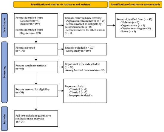
Figure 1.
Flow diagram for the systematic review.
2.2. Research Questions
- RQ1: How do various heuristic methods (e.g., Genetic Algorithms, Particle Swarm Optimization, Adaptive PSO, etc.) compare in performance when correlating reduced thermal mathematical models in spacecraft design?
- RQ2: How does parameter tuning influence both the convergence rate and overall performance of heuristic algorithms in thermal model correlation?
- RQ3: How do different heuristic methods perform when applied to the reduction of thermal models with varying complexity (e.g., simple vs. complex models)?
From these questions, the search terms used in Table 2 were found, with the results shown.
Table 2.
Terms used in the databases.
2.3. Criteria
Exclusion and inclusion criteria were applied to refine the selection of 24 papers from the initial pool. The Rayyan tool was used to automatically detect articles that were either partially or entirely (100%) duplicated. This tool allows for the removal of duplicates or the retention of multiple copies if necessary.
Exclusion criteria are the following:
- Did not involve the direct application of heuristic methods for global optimization;
- Were unrelated to the correlation of thermal models in the aerospace industry.
Inclusion criteria are the following:
- Focused on the reduction or test correlation of a thermal model;
- Addressed aerospace thermal modeling;
- Applied heuristic methods directly to the global optimization of the correlation process.
2.4. Data Extraction Method
- Identify which heuristic method was used on the test correlation or model reduction case study, as well as when and where it was used (addressing RQ1);
- Identify the fitness function equation used for test correlation or model reduction (addressing RQ2);
- Identify the parameters tuning values used for test correlation or model reduction (addressing RQ2);
- Identify if thermal model size is considered to be simple or complex (addressing RQ3).
2.5. Analysis
As shown in Figure 2a and Table 3, a total of N = 24 published documents (from journals and conferences) were identified between 2007 and 2024. Although only a few papers were published in the early years, the number of publications has increased significantly after 2022, indicating growing attention to the subject.
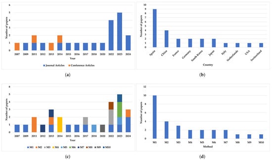
Figure 2.
Number of studies/publications of the systematic review: (a) total of N = 24 published documents (journals and conferences) were identified between 2007 and 2024. (b) Geographical distribution of the publications. (c) Methods implemented of the publications between 2007 and 2024. (d) Most implemented method detailed in Table 4.
Table 3.
Articles published in recent years (for N = 24 papers).
The geographical distribution of these publications is illustrated in Figure 2b, with Spain leading the contributions with nine publications, followed by China with four.
Regarding the methods implemented, Figure 2c shows that the N = 24 documents employed a total of 28 methods (with some papers using more than one method) during this period. Furthermore, when counting the number of publications per method, as depicted in Figure 2d, Genetic Algorithms (M1) emerge as the most frequently used method with 10 publications, followed by the Gradient-based Algorithm (M2), as detailed in Table 4.
Table 4.
Most used methods (for N = 24 papers with 28 implementations; some papers have more than 1 method implemented).
2.6. Implementing Heuristic Methods
It was decided to compile an expanded list of heuristic methods to gain a more comprehensive understanding of the topic addressed in this paper. This list was constructed by combining the heuristic methods referenced in the literature review presented in Section 2 with selected methods from the PRISMA systematic review approach described in Section 2.5. Since the global optimization methods applied to thermal models during the reduction and correlation process are often difficult to understand or differentiate, given that many papers do not clearly explain their underlying mechanisms, some methods were excluded. Specifically, the Bayesian Algorithm, Conductance Matrix Fitting, and Jacobian Propagation were omitted. In addition, the machine learning approach was excluded because it is not strictly considered a heuristic method. Furthermore, certain methods exhibit similarities (e.g., Gradient-based Algorithms and simulated annealing [31]) and therefore simulated annealing is considered instead.
Table 5 below provides a summary, in table format, of only the heuristic methods. The table lists each algorithm’s name, its source, the publication year, the adjustable parameters, and references to thermal modelling studies that have employed the respective method.
Table 5.
Summary of optimization algorithms, their parameters, and thermal modeling references.
As shown in Table 5, there are a 26 selected heuristic methods in this review table and only 8 methods mentioned in the literature have been directly applied, leaving 18 without any of mention of application in thermal model correlation or reduction. This means that 65% of the presented algorithms in Table 5 were never mentioned or used for thermal model correlation or reduction purposes, leading into a big gap in knowledge which this work wishes to address and solve. In this document, we addressed the study of how each one of these global optimization methods in Table 5 performs against a thermal model correlation and reduction process.
3. Heuristic Methods on a Simple Thermal Model Reduction and Correlation
3.1. Reduction and Correlation Process
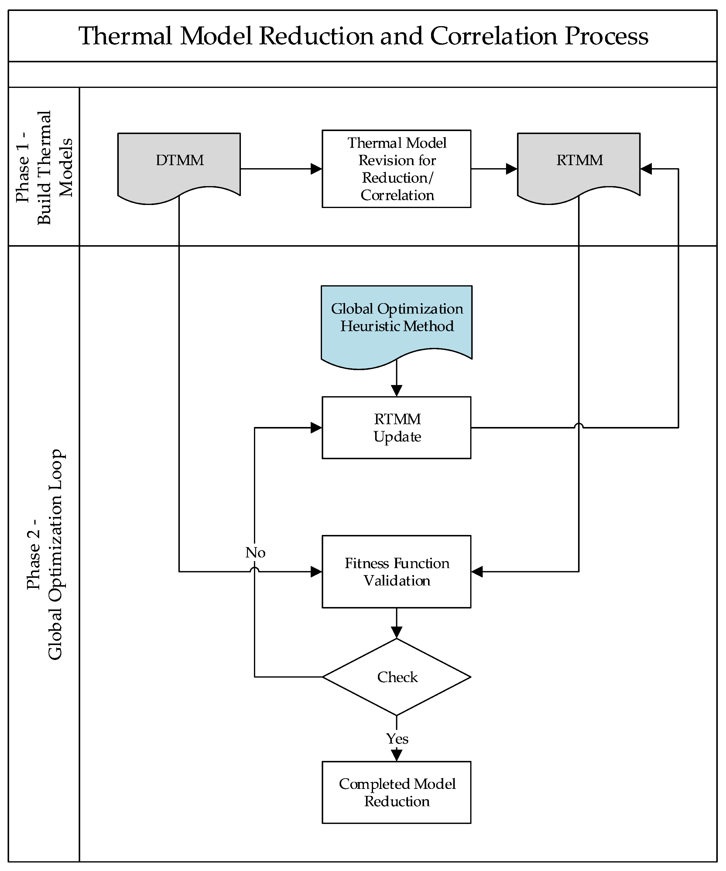
The application of a heuristic method for global optimization in the thermal model reduction and correlation process is structured in two distinct phases, as illustrated in Figure 3: Phase 1—Build Thermal Models and Phase 2—Global Optimization Loop.

Figure 3.
Workflow diagram of a heuristic methods on thermal model reduction and correlation.
In Phase 1, the process begins with the development of both the detailed thermal mathematical model (DTMM) and the reduced thermal mathematical model (RTMM). These models are created and arranged to enable comparison and correlation. An initial revision of the RTMM is conducted to prepare it for reduction and alignment with the DTMM. Phase 2 encompasses an iterative global optimization loop aimed at minimizing the discrepancy between the DTMM and RTMM outputs. A global heuristic optimization method is applied to guide adjustments to the RTMM parameters. Each iteration involves updating the RTMM, validating its performance through a comparison against the DTMM using a fitness function, and checking whether the predefined convergence criterion is met. This criterion—often referred to as a “fitness function” [2,4,5,6,14,17,20,59], “objective function” [16,21,40], or “error function” [22]—quantifies the accuracy of the RTMM relative to the DTMM. The loop continues until the fitness function indicates that the model meets the correlation acceptance criteria. Once this condition is satisfied, the process concludes with a validated and reduced thermal model.
Generally, this “fitness function” is defined as something similar to the root sum square of all selected nodes between DTMM and RTMM. The equations are generally written as follows [2,17,21]:
where .
These equations demonstrate that typical fitness functions evaluate root sum square of differences between corresponding DTMM and RTMM nodes.
Once the fitness function between the DTMM and RTMM is defined, it implements the heuristic loop method to iteratively optimize the adjustable parameters of the RTMM.
The process operates in a loop:
- Adjust the parameters by updating the RTMM;
- Run thermal simulations for RTMM;
- Evaluate the fitness function.
This optimization is carried out using a heuristic method, such as a Genetic Algorithm, simulated annealing, or other optimization techniques, as shown in Table 5. The goal is to minimize the fitness function, ideally reducing it to zero, thereby achieving a high degree of correlation between the DTMM and RTMM.
3.2. Simple Model—Thermal Mathematical Models
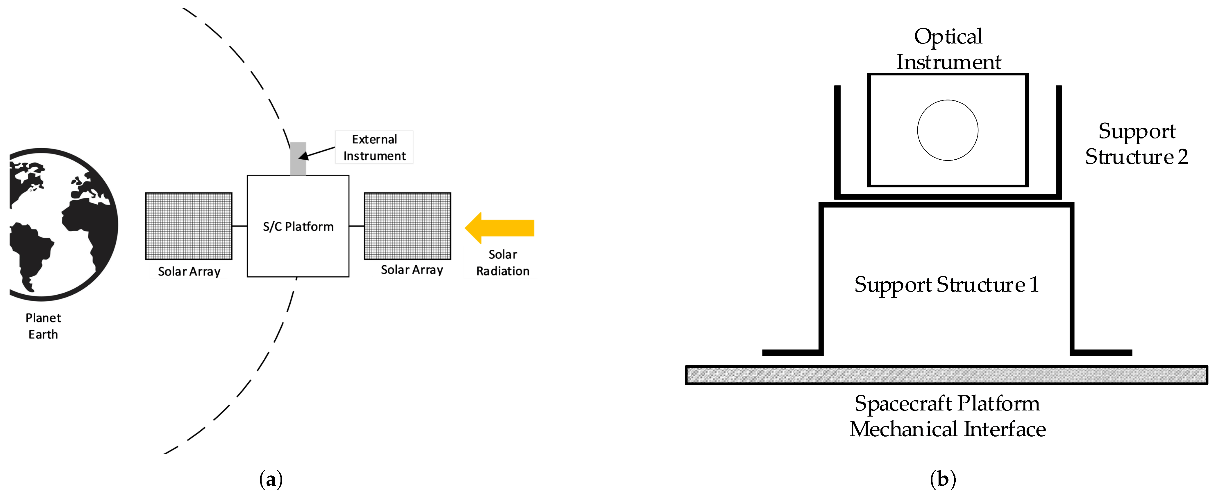
The thermal model represents an optical instrument mounted on an external panel of a satellite operating in low Earth orbit (LEO). As shown in Figure 4a, the satellite is depicted using a simple schematic for an external instrument configuration, orbiting the Earth with a 90-min period. During its orbit, the satellite is exposed to solar radiation when it is outside Earth’s shadow, while the external panel radiates heat into deep space and exchanges thermal energy with the satellite’s internal components.
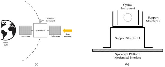
Figure 4.
Aerospace instrument concept design illustration: (a) orbit of a satellite with an external instrument. (b) External instrument concept design where the Spacecraft Platform Mechanical Interface is attached to Support Structure 1, which is connected to Support Structure 2, which supports the Optical Instrument at its top.
Figure 4b illustrates the instrument concept design. In this design, the Spacecraft Platform Mechanical Interface is attached to Support Structure 1, which is connected to Support Structure 2, which supports the Optical Instrument at its top. This generic configuration was selected because it typifies the design commonly used for optical instruments on satellites.
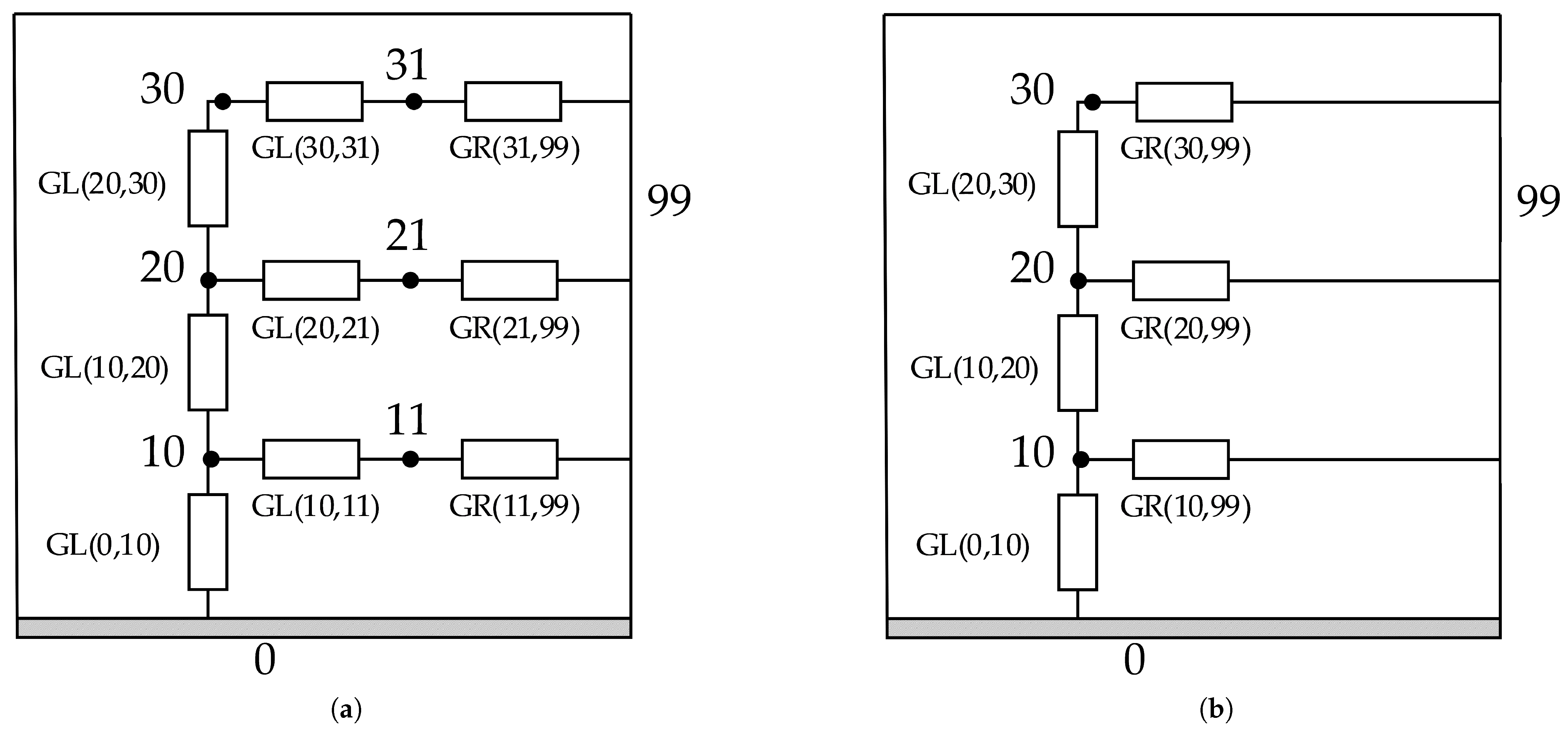
Figure 5a,b present the Thermal Resistance Networks for the detailed thermal mathematical model (DTMM) and the reduced thermal mathematical model (RTMM), respectively. Although the DTMM shown in Figure 5a is already a simplified thermal model, it is still referred to as the “detailed” model in this study because it serves as the reference for evaluating the reduced model’s accuracy. As discussed in the Introduction (Section 1) and similar to the approach by Klement [17], it is necessary to define both a reference model (DTMM) and a reduced model (RTMM), where the RTMM has fewer nodes but still captures the key thermal behaviour of the DTMM. Despite the simplicity of the DTMM, the process of reducing and correlating the RTMM is difficult.
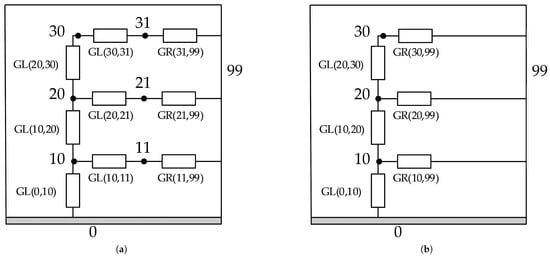
Figure 5.
Thermal Resistance Networks for (a) detailed TMM; (b) reduced TMM.
3.3. Mathematical Description
The two thermal models simulate transient temperature behavior under conductive, radiative, and solar power inputs. The DTMM treats internal and surface nodes separately, whereas the RTMM uses a lumped parameter approach by combining each internal node with its corresponding surface node. The nodes considered are as follows:
- Internal Nodes: 10, 20, 30
- Surface Nodes: 11, 21, 31
3.4. DTMM Equations
3.4.1. Internal Nodes (10, 20, 30)
The temperature evolution for the internal nodes is governed by conduction between the ambient and neighboring nodes, as well as internal power input:
3.4.2. Surface Nodes (11, 21, 31)
The surface nodes experience both conduction from their associated internal nodes and radiative heat transfer:
3.5. RTMM Equations
In the reduced model, each internal–surface pair is lumped into a single effective node. The energy balance for each lumped node incorporates both the conduction and radiative terms, as well as the total power input.
3.5.1. Lumped Node 10–11
3.5.2. Lumped Node 20–21
3.5.3. Lumped Node 30–31
3.6. Solar Power Input
The solar power input at each node varies sinusoidally over time. The input for each node i is given by
where for DTMM and for the RTMM.
3.7. Model Parameters
3.7.1. Physical Constants
- Stefan-Boltzmann constant: ;
- Solar constant: ;
- Solar absorptivity: ;
- Orbit period: .
3.7.2. Node Masses and Specific Heat
- Specific heat capacities: ;
- Masses of the nodes: .
3.7.3. Thermal and Radiative Properties
- Emissivities: ;
- Radiative areas: ;
- Thermal conductances: ;
- Satellite mechanical interface temperature: ;
- Space radiative interface temperature: .
A short summary of both thermal models, the DTMM considers separately the internal nodes (10, 20, 30) and surface nodes (11, 21, 31), including both conductive and radiative heat transfer. Regarding the RTMM, it combines each internal–surface node pair (10–11, 20–21, 30–31) into a single lumped node, simplifying the analysis while retaining the essential thermal dynamics.
Both systems of ordinary differential equations (ODEs) can be solved numerically (e.g., using odeint from the scipy library) to obtain transient temperature profiles.
3.8. Global Optimization Method Implementation
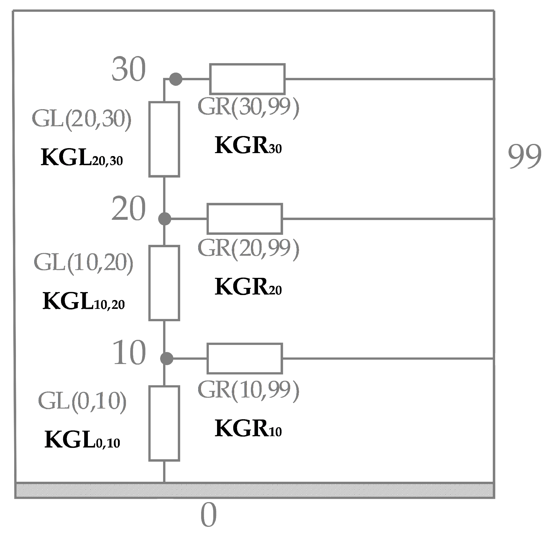
To improve the thermal model correlation between the DTMM and RTMM, it is necessary to add adjustable variables“KGL” and “KGR”, labelled as , , , , , and , which are incorporated into the RTMM, as illustrated in Figure 6.
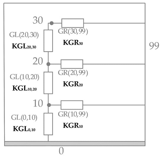
Figure 6.
RTMM with adjustable variables “KGL” and “KGR”—resistance network.
To optimize these “KGL” and “KGR” values for achieving the lowest possible FF, a heuristic global optimization method (as summarized in Table 5) must be implemented. By refining these parameters, the RTMM can be correlated more closely with the DTMM.
The implementation of a global optimization method to optimize the “KGL” and “KGR” variables in RTMM—namely,
is shown in Figure 6.
Each heuristic global optimization methods listed in Table 5 to determine which approach is most effective for the Thermal Model Reduction and Correlation Process between DTMM and RTMM. However, before directly comparing these methods, we first need to adjust each method’s configuration “parameters” (e.g., population size, mutation rate, initial temperature, cooling rate, etc.).
To that end, we used a Genetic Algorithm to optimize the parameters of each method within a 20-generation loop, enabling stabilization of each method’s configuration parameters and thereby making them comparable. In each iteration of this 20-generation loop, every method was run for 50 iterations/generations. Because running all methods for a large number of iterations is time-consuming, 20 iterations/generations was selected as the most balanced compromise. Consequently, each optimized algorithm was run for a total of 400 iterations/generations overall.
However, several methods were excluded from this benchmark for the following reasons:
- Broyden: This method primarily depends on the “tolerance” and “Max Iterations” parameters. The “tolerance” was already set to a very low value (∼), which is not easily optimized. Additionally, “Max Iterations” must be set relatively high because the method requires initializing a Jacobian matrix, making it more difficult to compare with other methods. However, this method could be revised and implemented in later complex models.
- Memetic Algorithm (MA): This algorithm is essentially based on the Genetic Algorithm (GA), making it redundant to run separately.
- Distributed Search (DS): The DS method uses the GA as a baseline, adding parallel agents to search for other local minima. Since the GA has already been analyzed, DS was not implemented.
- Multi-Objective Optimization (GA based): Although similar to the GA, this approach requires more than one fitness function to be effective, which was beyond the scope of this study.
- Monte Carlo Hybrid Algorithm: This method proved to be significantly more time-consuming than the others. One key limitation of the Monte Carlo approach is that it lacks the adaptive learning mechanisms present in other optimization algorithms. Instead, it performs a blind search around the current best solution using a fixed “search radius” parameter. If this radius is too small, the method fails to explore the solution space adequately, if it is too large, it often samples poor-quality regions, reducing efficiency. An adaptive or dynamic adjustment of the search radius could potentially improve performance, but due to constraints in computational resources and time, it was not feasible to explore such enhancements or run the method for a sufficient number of iterations to ensure convergence.
- Machine Learning: Machine learning itself is not a heuristic global optimization method, but it frequently employs such methods for optimization tasks; however it will not be used in this study. This method will be implemented in future studies.
A total of 21 methods were optimized and compared, as shown in the following sections.
4. Results
4.1. DTMM vs. RTMM: Without Correlation
All nodes are initialized at 25 °C. The simulation covers 24 h, divided into 5000 time steps. The ODE system is solved using odeint from scipy.integrate. The simulation was run on the SPYDER IDE using an AMD 5900X CPU with 64 GB of RAM.
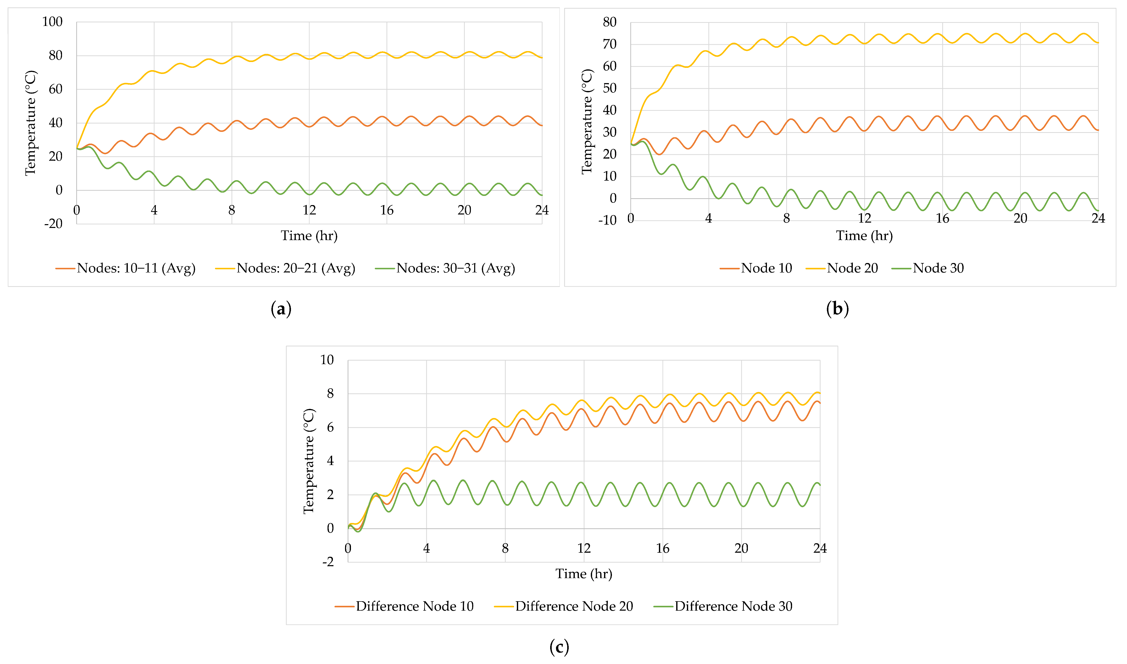
The detailed TMM simulation results are presented in Figure 7a. This figure displays the transient average temperatures (mass-weighted) for each node pair (e.g., 10–11, 20–21, and 30–31) over a 24 h orbit. These results offer a comprehensive view of the system’s thermal behaviour, emphasizing the dynamic interplay between conduction, radiation, and solar input.
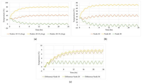
Figure 7.
Simulation temperature results without correlation: (a) DTMM. (b) RTMM. (c) Difference between DTMM and RTMM.
Despite the 90 min exposure to solar radiation during each orbital period, the nodes ultimately reach equilibrium temperatures. Specifically,
- Nodes 10–11 stabilize at an average temperature of approximately 41 °C.
- Nodes 20–21 stabilize at an average temperature of approximately 80.25 °C.
- Nodes 30–31 stabilize at an average temperature of approximately 0 °C.
It is important to note that the temperatures shown in Figure 7a primarily reflect the behaviour of Nodes 10, 20, and 30, which together account for 90% of the system’s total mass (30 kg) relative to the overall system mass of 33 kg. This mass distribution naturally causes the thermal characteristics of these nodes to dominate the system’s response.
The reduced TMM simulation results of the Simple Model are presented in Figure 7b. This figure displays the transient temperatures for each node (e.g., 10, 20, and 30) over a 24 h orbit. These results offer a comprehensive view of the system’s thermal behaviour, emphasizing the dynamic interplay between conduction, radiation, and solar input.
Despite the 90 min exposure to solar radiation during each orbital period, the nodes ultimately reach equilibrium temperatures. Specifically,
- Node 10 stabilizes at an average temperature of approximately 34.31 °C.
- Node 20 stabilizes at an average temperature of approximately 72.86 °C.
- Node 30 stabilizes at an average temperature of approximately −1.41 °C.
A comparison of the temperature results for Nodes 10, 20, and 30 between the detailed and reduced TMMs is presented in Figure 7c.
Initially, both models start at the same temperature of 25 °C, as they share identical initial conditions. As a result, the temperature difference between the detailed and reduced TMMs is 0 °C at the start of the simulation ( s), as shown in Figure 7c.
As the simulation progresses, temperature differences between the two models begin to emerge. These differences increase over time but eventually stabilize at steady-state conditions. The steady-state average temperatures for each node are as follows:
- Node 10 temperature difference stabilizes at an average of approximately 6.5 °C.
- Node 20 temperature difference stabilizes at an average of approximately 7.7 °C.
- Node 30 temperature difference stabilizes at an average of approximately −2.0 °C.
These temperature difference results in Figure 7c were obtained without any adjustments applied to either the DTMM or RTMM.
Because the DTMM features the highest number of nodes and, therefore, provides the most detailed results, its output is considered the temperature reference value. This assumption mirrors the approach used during thermal test correlations, where measured thermal test data serve as the “temperature reference,” and the thermal model is refined accordingly to match those reference values.
In addition to examining the temperature differences between the DTMM and RTMM, it is also important to evaluate a global fitness value. Following Equation (2) as the baseline example, the fitness function sums the root-sum-square (RSS) of the temperature differences for each set of nodes across the entire simulation period, as shown in Equation (17):
Using the temperature differences presented in Figure 7c and no model correlation, the calculated fitness function is .
To achieve a better (i.e., lower) value, a thermal model correlation must be performed by optimizing the adjustable variables mentioned in Section 3.8, Figure 6, namely , that scale the thermal conductors (GLs) or thermal radiative conductors (GRs). These adjustable variables are tuned to achieve the best possible correlation.
4.2. Heuristic Method Benchmark Results
As previously mention in Section 3.8, a Genetic Algorithm was used to optimize the parameters of each heuristic method within a 20-generation loop, enabling a stabilization of each method’s configuration “parameter” approximation and therefore making them comparable. In each iteration of this 20-generation loop, every method was run for 50 iterations/generations. Because running all methods for a large number of iterations is time-consuming, 20 iterations/generations was selected as the most balanced compromise. Consequently, each optimized algorithm was run for a total of 400 iterations/generations overall. Since 21 heuristic methods were optimized, here the optimization of the most used method, the Genetic Algorithm, is presented.
Cultural Algorithm Parameter Convergence Results
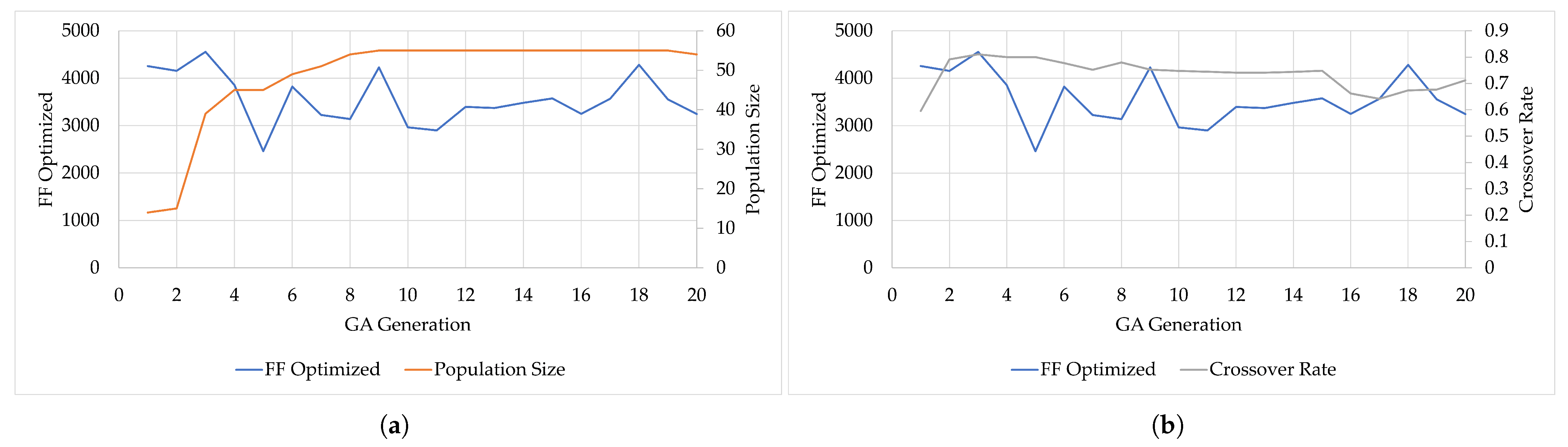
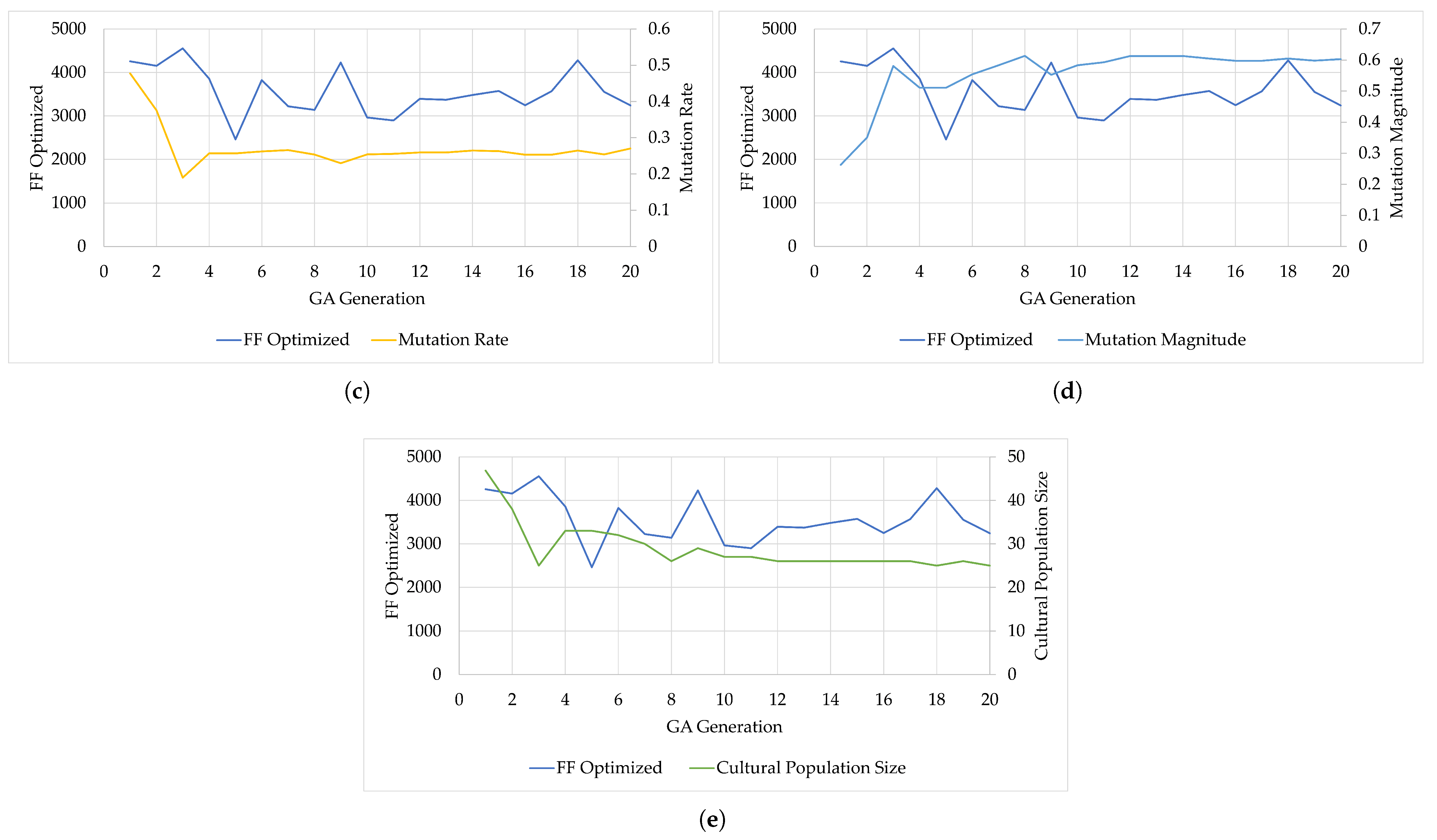
Here is presented the Cultural Algorithm (CA) method convergence on the configuration parameters. The evolution of such parameters can be found in Figure 8a for “Population Size”, Figure 8b for “Crossover Rate”, Figure 8c for “Mutation Rate”, Figure 8d for “Mutation Magnitude”, and Figure 8e for “Cultural Population Size”. Figure 8 also illustrates how the changes over the course of 20 generations of the Genetic Algorithm optimization process, along with the other parameters.
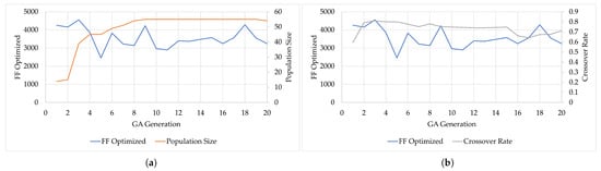
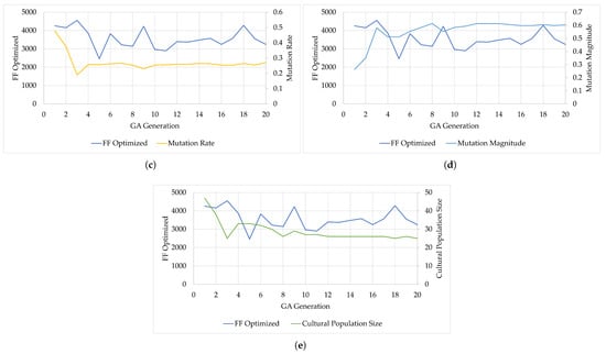
Figure 8.
Evolution of and respective parameters for Cultural Algorithm (CA): (a) Population Size. (b) Crossover Rate. (c) Mutation Rate. (d) Mutation Magnitude. (e) Cultural Population Size.
The same optimization process was performed for all 21 heuristic methods described in Table 5. In this section is presented a summary of the results in table format from the previous plots for all 21 heuristic methods.
4.3. Heuristic Methods Benchmark Results
4.3.1. Parameters Optimization Results
The following table presents the Boxplot statistical elements for each method configuration “Parameter”. This is based on the six-number summary, which includes the minimum, maximum, average, median, and the first and third quartiles, for each “Parameter”.
The results presented here in Table 6 show how is statistical distributed the “Parameters” in each method.
Table 6.
Boxplot statistical elements—heuristic method “parameters”.
Next, Figure 9 shows the average time per generation/iteration for each method. The data indicate that some methods are faster than others (e.g., Simulated Annealing and Alienor). On average, each generation/iteration takes approximately 45 s when using the minimum parameter values from Table 7. If the maximum parameter values are used, the time per generation increases by roughly 2.5 times, reaching approximately 108 s. These differences can be significant in correlation processes that involve hundreds of generations or iterations. In addition to computation time, memory usage was also evaluated. The implementation of these methods exhibited relatively low memory demands on current computing systems, with a maximum observed peak of 233 MB. Therefore, memory usage does not present a significant concern. However, as will be seen in Section 4.3.2, the fastest method does not necessarily yield the lowest .
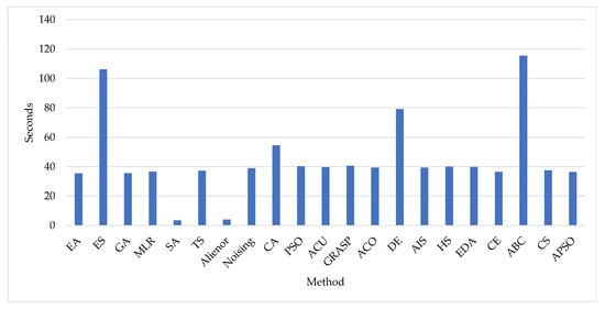
Figure 9.
Average time per generation/iteration for each method.
Table 7.
Heuristic method boxplot statistical elements: fitness function .
4.3.2. Fitness Function Results
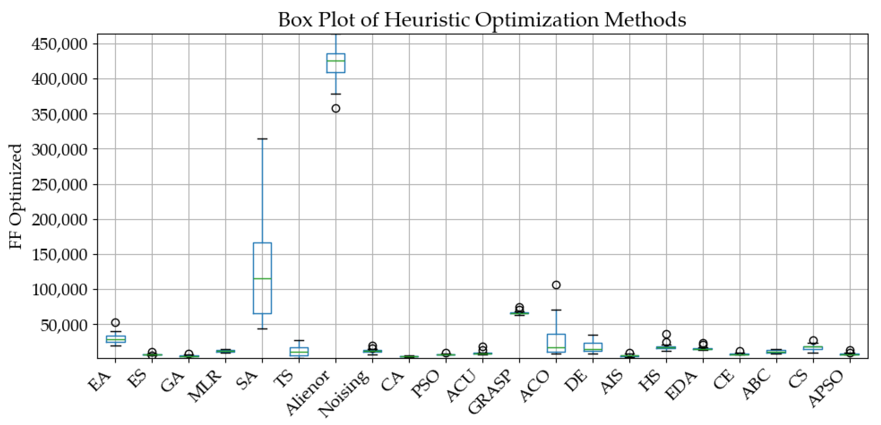
The following table presents a statistical analysis of the outcomes, illustrated using a standardized boxplot, using the six-number summary, which includes the minimum, maximum, average, median, and the first and third quartiles.
The respective boxplot charts are presented in Figure 10.
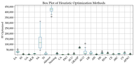
Figure 10.
Boxplot chart—fitness function .
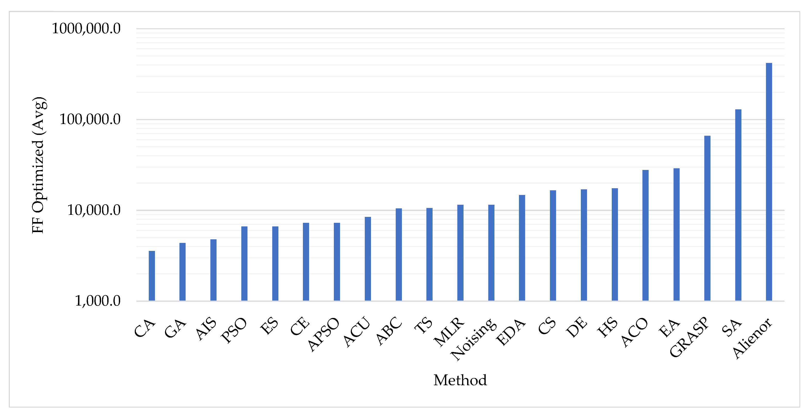
As a simple visual analysis of , the average comparison plot is presented in Figure 11 for the tested methods, illustrating that the Cultural Algorithm (CA) method achieves the best performance, while the Alienor method demonstrates the poorest performance.
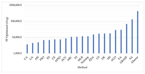
Figure 11.
average for each heuristic method.
4.3.3. Best Fitness Function Results
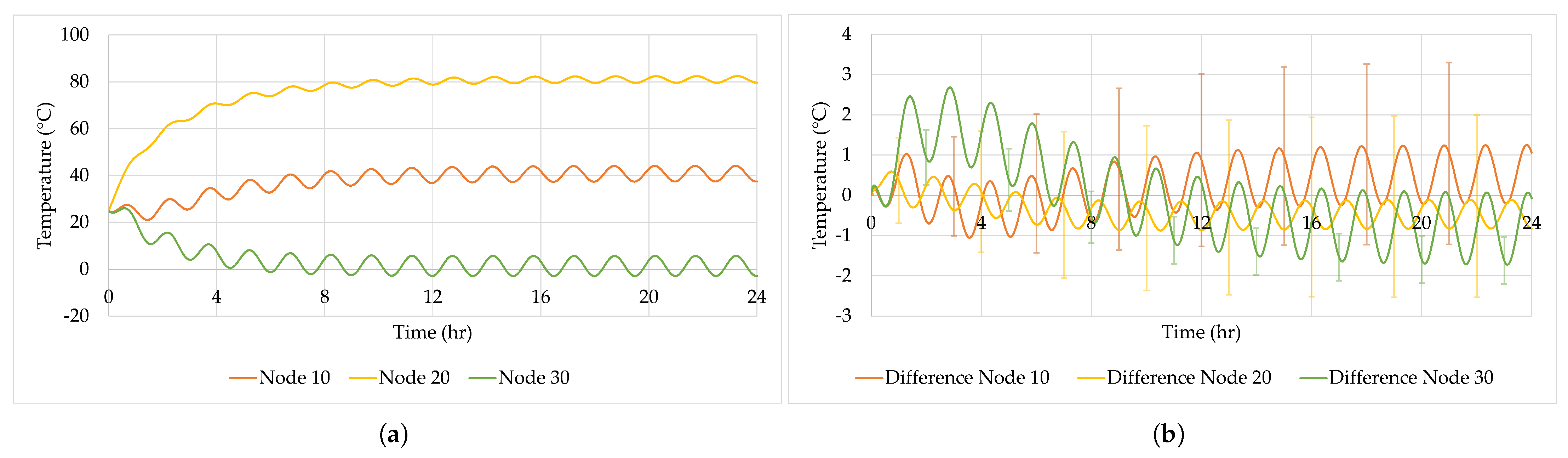
The best correlated reduced TMM simulation results of the Simple Model are presented in Figure 12a,b, where the simulation temperature results and temperature differences between DTMM and RTMM, respectively, are presented Additionally, the uncertainty of the RTMM was assessed by changing the model parameters, i.e., node mass and emissivity, with a variation of ±5%, for each node. The uncertainty was estimated with Equation (18).
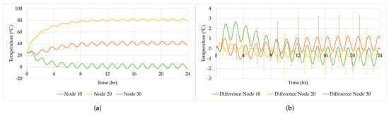
Figure 12.
Correlated RTMM with Cultural Algorithm (CA) with lowest value: (a) RTMM temperature results. (b) Temperature difference between DTMM and RTMM, including the model uncertainty.
This figure displays the transient temperatures for each node (e.g., 10, 20, and 30) over a 24 h orbit, similar to Section 4.1. However, now these results have already been correlated with the DTMM results. This correlation was made by using the Cultural Algorithm (CA) best correlation adjustment factors from a previous optimization exercise. These adjustment factors, and , are now:
- ;
- ;
- ;
- ;
- ;
- .
Despite the 90 min exposure to solar radiation during each orbital period, the nodes ultimately reach equilibrium temperatures, as shown in Figure 12a. Specifically;
- Node 10 stabilizes at an average temperature of approximately 40.68 °C.
- Node 20 stabilizes at an average temperature of approximately 80.98 °C.
- Node 30 stabilizes at an average temperature of approximately −1.34 °C.
Similar to the analysis conducted in Figure 7c, where temperature differences between the DTMM and RTMM were compared without any RTMM model corrections or correlations, we now examine the temperature differences with optimization applied. The new results show significantly smaller temperature differences, as shown in Figure 12b.
As in the previous comparison in Section 4.1 realtive to Figure 7c, both models begin at the same initial temperature of 25 °C due to identical initial conditions.
As the simulation progresses, temperature differences between the two models begin to emerge. These differences increase over time but eventually stabilize at steady-state conditions. The steady-state average temperatures for each node are as follows:
- Node 10 temperature difference stabilizes at an average of approximately 0.55 °C ± 2.8 °C.
- Node 20 temperature difference stabilizes at an average of approximately −0.46 °C ± 2.4 °C.
- Node 30 temperature difference stabilizes at an average of approximately −0.77 °C ± 1.8 °C.
These temperature differences in Figure 12b were obtained with adjustments applied to the RTMM, using the Cultural Algorithm (CA) optimization method, which achieved the fitness function value of . It is also interesting to note that the RTMM uncertainty due to variations in mass and external surface emissivity within ±5% shows that it is possible to exceed the 3 °C limit specified in typical standards [1]. This exceedance of the 3 °C limit could be considered significant; however, it does not imply that the difference between the DTMM and RTMM is on the order of 3 °C, which is still considered very low.
5. Discussion
This study has made significant advancements in the application of heuristic global optimization methods for reducing and correlating thermal models in aerospace applications. The discussion is structured into several key areas.
5.1. Literature Review
As illustrated in Figure 2a and Table 3, the PRISMA analysis identified 24 published documents (from journals and conferences) between 2007 and 2024. Although publications were sparse in the early years, a significant increase after 2022 indicates growing interest in this field.
The geographical distribution of these publications, shown in Figure 2b, highlights Spain as the leading contributor (nine publications), followed by China (four publications).
Regarding the methods implemented, Figure 2c shows that the 24 documents employed 28 methods, with some studies utilizing multiple approaches. When analysing the number of publications per method (Figure 2d), Genetic Algorithms (GAs) emerged as the most frequently used technique, appearing in ten publications, followed by Gradient-Based Algorithms, as detailed in Table 4.
After the PRISMA systematic review, a compilation of existing heuristic methods available was performed on the literature and then summarized in Table 5, where it presents a list of 26 heuristic methods identified in the literature. However, only eight methods were explicitly mentioned as being applied to thermal model correlation or reduction. This means that 65% of the methods listed remain unexplored, highlighting a significant knowledge gap. This study aims to bridge this gap by evaluating the performance of these global optimization methods in thermal model correlation and reduction.
5.2. Interpretation of Simulation Results
The numerical simulations demonstrate that heuristic methods—particularly Cultural Algorithms (CAs), Genetic Algorithms (GAs), and Artificial Immune Systems (AISs)—effectively reduce discrepancies between the detailed and simplified thermal models. The observed convergence and temperature differences below 3 °C in transient simulations confirm their ability to handle complex, nonlinear parameter spaces. These findings suggest that heuristic approaches can serve as a robust alternative to traditional, manually tuned methods in thermal correlation analysis.
A key aspect of this discussion concerns parameter tuning in heuristic methods. In this study, a Genetic Algorithm (GA) optimization process was employed to fine-tune parameters across different heuristic techniques. The goal was to establish a more systematic and comparable optimization loop for each method, enabling a more natural convergence of the parameter tuning and then a better performance comparison based on fitness function () values.
Some heuristic methods, e.g., the CA, GA, and AIS, share common parameters, such as: “Population Size”, “Mutation Rate”, and “Mutation Magnitude”.
However, others have unique parameters that are not directly comparable across methods, such as Cultural Population Size (specific to CAs) and Clone Factor (specific to AISs).
If we compare the common parameters, we find the following:
- Population Size: 49 (CA), 43 (GA), and 21 (AIS). While the CA and GA are similar, the AIS has a significantly smaller value.
- Mutation Rate: 0.271 (CA), 0.299 (GA), and 0.268 (AIS), indicating close similarity.
- Mutation Magnitude: 0.557 (CA), 0.582 (GA), and 0.667 (AIS), with the AIS showing a difference.
Despite similarities in some tuning parameters, significant differences emerge in others, such as Population Size. Additionally, unique parameters specific to each method make direct comparisons challenging. To address this, we compiled a comprehensive statistical dataset for each heuristic method. This dataset serves as a reference for researchers and practitioners looking to apply heuristic methods to thermal model correlation, providing insights into acceptable parameter ranges and expected optimization behaviours.
5.3. Strengths and Limitations
While the results are promising, it is essential to acknowledge both strengths and limitations.
Strengths
- The methods demonstrate high accuracy and effective convergence, making them well suited for handling non-linearity in thermal models.
- The approach offers a structured methodology for automating and improving parameter tuning, reducing reliance on manual adjustments of the methods of tuning parameters.
Limitations:
- Selecting the optimal tuning parameters for each method requires extra computational cost, which can lead to increased computational time.
- These findings are based on a simplified thermal model; further validation is needed for larger and more complex aerospace systems.
5.4. Implications for Future Research
This work establishes a robust global heuristic framework for thermal model reduction and correlation. To broaden its applicability and validate its performance under realistic conditions, future investigations should explore the following directions:
- Laboratory Validation. Develop and instrument a representative thermal test setup (e.g., a multi-plate panel or electronics mock-up) equipped with temperature sensors. Conduct experiments in a controlled environment and compare the measured temperature profiles with predictions from both the DTMM and RTMM to evaluate accuracy and convergence behaviour.
- Larger Model Scaling. Apply the reduction methodology to more complex aerospace thermal networks, such as complete satellite buses or payload assemblies with hundreds of nodes, to assess scalability, accuracy, and computational efficiency.
6. Conclusions
This study has explored the application of heuristic global optimization methods for thermal model reduction and correlation in aerospace applications. The key contributions of this work are summarized below.
- Comprehensive Literature Review: A systematic review of 24 publications from 2007–2024 identified 26 heuristic optimization methods, highlighting a significant gap in the application of many techniques.
- High-Accuracy Correlation: The application of heuristic methods resulted in temperature discrepancies below 3 °C under transient conditions, demonstrating their effectiveness in improving model accuracy.
- Comparative Evaluation of Methods: While Genetic Algorithms (GAs) have been the dominant approach since Jouffroy’s pioneering work in 2007, this study highlights that other methods—such as Cultural Algorithms (CAs) and Artificial Immune Systems (AISs)—can perform competitively.
In conclusion, this study confirms that heuristic global optimization methods are effective for thermal model reduction and correlation in aerospace engineering. These findings contribute to both theoretical understanding and practical applications, providing a solid foundation for improving thermal model accuracy and optimization processes in complex engineering systems.
Author Contributions
Conceptualization, J.P.C. and B.N.A.; methodology, J.P.C. and B.N.A.; software, J.P.C.; validation, R.M. and P.G.; investigation, J.P.C.; resources, R.M.; data curation, J.P.C.; writing—original draft preparation, J.P.C.; writing—review and editing, R.M. and P.G.; visualization, J.P.C. and B.N.A.; supervision, R.M., P.G., and A.R.R.S.; project administration, R.M. and P.G.; funding acquisition, R.M. All authors have read and agreed to the published version of the manuscript.
Funding
The authors acknowledge the support provided by the Research project called Mobilising Agenda: New Space Portugal (Ref. C644936537-00000046, Notice ACC02/CO5-i01/2022), funded by the “Mobilising Agendas for Business Innovation” through the “Recovery and Resilience Programme (PRR)”. The authors acknowledge Fundação para a Ciência e a Tecnologia (FCT) for its financial support via the projects LAETA Base Funding (DOI: 10.54499/UIDB/50022/2020), LAETA Programmatic Funding (DOI: 10.54499/UIDP/50022/2020). The authors acknowledge Fundação para a Ciência e a Tecnologia (FCT) for its financial support via the projects: LIP Base Funding (UID/50007/2023).
Institutional Review Board Statement
Not applicable.
Informed Consent Statement
Not applicable.
Data Availability Statement
The raw data supporting the conclusions of this article will be made available by the authors on request.
Conflicts of Interest
The authors declare no conflicts of interest.
Abbreviations
The following abbreviations are used in this manuscript:
| Area of Node i (m2) | |
| Solar Absorptivity of Node i | |
| ABC | Artificial Bee Colony |
| ACU | Approximate Convex Underestimation |
| ACO | Ant Colony Optimization |
| AIS | Artificial Immune Systems |
| APSO | Adaptative Particle Swarm Optimization |
| CA | Cultural Algorithms |
| CE | Cross-Entropy Method |
| CoI | Conflict of Interest |
| CPU | Central Processing Unit |
| Specific Heat at Constant Pressure (J/kg.K) | |
| DE | Differential Evolution |
| DTMM | Detailed Thermal Mathematical Model |
| DS | Distributed Search |
| EA | Evolutionary Algorithm |
| EDA | Estimation of Distribution Algorithms |
| ES | Evolutionary Strategies |
| Emissivity of Node i | |
| FF | Fitness Function |
| GA | Genetic Algorithm |
| GL | Conductive Thermal Conductance (W/°C) |
| GR | Radiative Thermal Conductance (W/°C) |
| GRASP | Greedy Randomized Adaptative Search Procedure |
| HS | Harmony Search |
| IDE | Integrated Development Environment |
| KGL | GL Adjustable Variable |
| KGR | GR Adjustable Variable |
| Heuristic Method n° # | |
| MA | Memetic Algorithms |
| MC | Monte Carlo Hybrid Algorithm |
| MDPI | Multidisciplinary Digital Publishing Institute |
| MLR | Multiple Linear Regression |
| MOOGA | Multiple-Objective Optimization GA Based |
| Mass of Node i (kg) | |
| NA | Not Available |
| N° of Thermal Nodes | |
| N° of Time Steps | |
| ODE | Ordinary Differential Equations |
| PRISMA | Preferred Reporting Items for Systematic Reviews and Meta-Analyses |
| PSO | Particle Swarm Optimization |
| Internal Heat Power on Node i (W) | |
| RAM | Random Access Memory |
| RQ# | Research Question n°# |
| RTMM | Reduced Thermal Mathematical Model |
| SA | Simulated Annealing |
| Solar Constant (W/m2) | |
| t | Time |
| Temperature of Node i (°C) | |
| Orbital Period | |
| TS | Tabu Search |
References
- ECSS-E-HB-31-03A; Space Engineering—Thermal Analysis Handbook, 1st ed. ESA Requirements and Standards Division: Noordwijk, The Netherlands, 2016; pp. 43–57.
- Jouffroy, F.; Durand, N. Thermal model correlation using Genetic Algorithms. In Proceedings of the 21st European Workshop on Thermal and ECLS Software, European Space Research and Technology Centre (ESTEC), Noordwijk, The Netherlands, 30–31 October 2007; pp. 125–138. [Google Scholar]
- John, J.H. Adaptation in Natural and Artificial Systems: An Introductory Analysis with Applications to Biology, Control, and Artificial Intelligence, 1st ed.; The MIT Press: Cambridge, MA, USA, 1992; pp. 1–232. [Google Scholar]
- THCOR-ASF-005-TN—Bibliography Study of Optimisation Methods with Focus on Genetic Algorithm Techniques w.r.t. Post-Test Thermal Model Correlation Problem. Available online: https://exchange.esa.int/restricted/model-correlation/ (accessed on 1 September 2024).
- THCOR-ASF-006-TN—Test Plan & Test Models for Verification of Post-Test Thermal Model Correlation by Using a Stochastic Global Optimisation Method. Available online: https://exchange.esa.int/restricted/model-correlation/ (accessed on 1 September 2024).
- THCOR-ASF-013-TN—Verification of Feasibility of Post-Test Thermal Model Correlation by Using Genetic Algorithms: Analysis of Test Plan Results. Available online: https://exchange.esa.int/restricted/model-correlation/ (accessed on 1 September 2024).
- Pintér, J.D. Continuous Global Optimization: A Personal Perspective. In Proceedings of the 40e Congrès Annuel de la SCRO, 40e Congrès Annuel de la SCRO, Montréal, QC, Canada, 26–29 April 1998; pp. 1–17. [Google Scholar]
- Dréo, J.; Pétrowski, A.; Taillard, E.; Siarry, P. Metaheuristics for Hard Optimization, 1st ed.; Springer: Berlin/Heidelberg, Germany, 2006; pp. 1–373. [Google Scholar]
- Harvatine, F.; DeMauro, F. Thermal Model Correlation Using Design Sensitivity and Optimization Techniques. In Proceedings of the 24th International Conference on Environmental Systems and 5th European Symposium on Space Environmental Control Systems, Friedrichshafen, Germany, 20–23 June 1994; pp. 1–11. [Google Scholar]
- Mareschi, V.; Perotto, V.; Gorlani, M. Thermal Test Correlation with Stochastic Technique. In Proceedings of the 35th International Conference on Environmental Systems (ICES), Rome, Italy, 11–14 July 2005; pp. 1–7. [Google Scholar]
- Momayez, L.; Dupont, P.; Delacourt, G.; Lottin, O.; Peerhossaini, H. Genetic algorithm based correlations for heat transfer calculation on concave surfaces. Appl. Therm. Eng. 2009, 29, 3476–3481. [Google Scholar] [CrossRef]
- Cheng, W.; Liu, N.; Li, Z.; Zhong, Q.; Wang, A.; Zhang, Z.; He, Z. Application study of a correction method for a spacecraft thermal model with a Monte-Carlo hybrid algorithm. Chin. Sci. Bull. 2011, 56, 1407–1412. [Google Scholar] [CrossRef]
- Palo, S.; Malosti, T.; Filiddani, G. Appendix Q Thermal Correlation of BepiColombo MOSIF 10 Solar Constants Simulation Test. In Proceedings of the 25th European Workshop on Thermal and ECLS Software, European Space Research and Technology Centre (ESTEC), Noordwijk, The Netherlands, 8–9 November 2011; pp. 125–138. [Google Scholar]
- Beck, T.; Bieler, A.; Thomas, N. Numerical thermal mathematical model correlation to thermal balance test using adaptive particle swarm optimization (APSO). Appl. Therm. Eng. 2012, 38, 168–174. [Google Scholar] [CrossRef]
- Kennedy, J.; Eberhart, R. Particle swarm optimization. In Proceedings of the ICNN’95—International Conference on Neural Networks, Perth, WA, Australia, 6 August 2002; pp. 1942–1948. [Google Scholar]
- van Zijl, N.; Zandbergen, B.; Benthem, B. Appendix G Correlating thermal balance test results with a thermal mathematical model using evolutionary algorithms. In Proceedings of the 27th European Space Thermal Analysis Workshop, European Space Research and Technology Centre (ESTEC), Noordwijk, The Netherlands, 3–4 December 2013; pp. 89–108. [Google Scholar]
- Klement, J. On Using Quasi-Newton Algorithms of the Broyden Class for Model-to-Test Correlation. J. Aerosp. Technol. Manag. 2014, 6, 407–414. [Google Scholar] [CrossRef]
- Klement, J. Appendix Q On using quasi Newton algorithms of the Broyden class for model-to-test correlation. In Proceedings of the 28th European Space Thermal Analysis Workshop, European Space Research and Technology Centre (ESTEC), Noordwijk, The Netherlands, 14–15 October 2014; pp. 213–228. [Google Scholar]
- Broyden, C.G. A class of methods for solving nonlinear simultaneous equations. Math. Comput. 1965, 19, 577–593. [Google Scholar] [CrossRef]
- Anglada, E.; Martinez-Jimenez, L.; Garmendia, I. Performance of Gradient-Based Solutions versus Genetic Algorithms in the Correlation of Thermal Mathematical Models of Spacecrafts. Int. J. Aerosp. Eng. 2017, 2017, 7683457. [Google Scholar] [CrossRef]
- Garmendia, I.; Anglada, E. Thermal Mathematical Model Correlation through Genetic Algorithms of an Experiment Conducted on Board the International Space Station. Acta Astronaut 2016, 122, 63–75. [Google Scholar] [CrossRef]
- Garmendia, I.; Anglada, E. Influence of the Measurements Uncertainties in the Correlation of Spacecraft Thermal Models against Thermal Results. Aerospace 2022, 9, 821. [Google Scholar] [CrossRef]
- Kang, J.; Kim, K.W.; Shin, S.; Kim, J.H. Efficient Correlation Method for Satellite Thermal Analysis Model Using Multiple Linear Regression and Optimization Algorithms. Int. J. Aeronaut. Space Sci. 2023, 24, 1257–1270. [Google Scholar] [CrossRef]
- Kim, J.-S.; Lee, S.; Kim, H.-K.; Kim, H.-D. Thermal Model Correlation of SNIPE Satellite Using Genetic-Algorithm-Based Multi-Objective Optimization Method. J. Spacecr. Rocket. 2023, 60, 1333–1342. [Google Scholar] [CrossRef]
- Preferred Reporting Items for Systematic Reviews and Meta-Analyses (PRISMA). Available online: https://www.prisma-statement.org/ (accessed on 15 February 2025).
- Kitchenham, B.; Charters, S. Guidelines for Performing Systematic Literature Reviews in Software Engineering; Technical Report; University of Durham: Durham, UK, 2007; Available online: https://legacyfileshare.elsevier.com/promis_misc/525444systematicreviewsguide.pdf (accessed on 18 May 2025).
- Kitchenham, B.; Brereton, O.P.; Budgen, D.; Turner, M.; Bailey, J.; Linkman, S. Systematic literature reviews in software en-gineering—A systematic literature review. Inf. Softw. Technol. 2009, 51, 7–15. [Google Scholar] [CrossRef]
- Rasool, G.; Ehsan, F.; Shahbaz, M. A systematic literature review on electricity management systems. Renew. Sustain. Energy Rev. 2015, 49, 975–989. [Google Scholar] [CrossRef]
- Viegas, J.L.; Esteves, P.R.; Melicio, R.; Mendes, V.M.F.; Vieira, S.M. Solutions for detection of non-technical losses in the electricity grid: A review. Renew. Sustain. Energy Rev. 2017, 80, 1256–1268. [Google Scholar] [CrossRef]
- Gonçalves, J.T.; Valtchev, S.S.; Melicio, R.; Gonçalves, A.; Blaabjerg, F. Hybrid three-phase rectifiers with active power factor correction: A systematic review. Electronics 2021, 10, 1520. [Google Scholar] [CrossRef]
- Kirkpatrick, S.; Gelatt, C.D.; Vecchi, M.P. Optimization by Simulated Annealing. Science 1983, 220, 671–680. [Google Scholar] [CrossRef]
- Torralbo, I.; Perez-Grande, I.; Sanz-Andres, A.; Piqueras, J. Correlation of Spacecraft Thermal Mathematical Models to Reference Data. Acta Astronaut. 2018, 144, 305–319. [Google Scholar] [CrossRef]
- Fogel, D.B. Artificial Intelligence Through Simulated Evolution, 1st ed.; Wiley-IEEE Press: Hoboken, NJ, USA, 1998; pp. 227–296. [Google Scholar]
- Vent, W. Rechenberg, Ingo, Evolutionsstrategie—Optimierung Technischer Systeme Nach Prinzipien Der Biologischen Evolution. 170 S. Mit 36 Abb. Frommann-Holzboog-Verlag, Stuttgart 1973, Broschiert. Feddes Repert. 1975, 86, 337. [Google Scholar]
- Fan, Y.; Feng, W.; Ren, Z.; Liu, B.; Huang, L.; Wang, D. Parameter Optimization of Thermal Network Model for Aerial Cameras Utilizing Monte-Carlo and Genetic Algorithm. Sci. Rep. 2022, 14, 22255. [Google Scholar] [CrossRef]
- Shin, S.; Lim, J.H.; Kim, C.-G. Thermal Parameter Determination in Underdetermined Spacecraft Thermal Models Using Surrogate Modelling. Acta Astronaut. 2024, 214, 583–592. [Google Scholar] [CrossRef]
- Anglada, E.; Garmendia, I. Correlation of Thermal Mathematical Models for Thermal Control of Space Vehicles by Means of Genetic Algorithms. Acta Astronaut. 2015, 108, 1–17. [Google Scholar] [CrossRef]
- Cui, Q.; Lin, G.; Cao, D.; Zhang, Z.; Wang, S.; Huang, Y. Thermal Design Parameters Analysis and Model Updating Using Kriging Model for Space Instruments. Int. J. Therm. Sci. 2022, 171, 107239. [Google Scholar] [CrossRef]
- Draper, N.R.; Smith, H. Applied Regression Analysis, 3rd ed.; Wiley: Hoboken, NJ, USA, 1998; pp. 668–669. [Google Scholar]
- Garmendia, I.; Anglada, E. Thermal Parameters Identification in the Correlation of Spacecraft Thermal Models against Thermal Test Results. Acta Astronaut. 2022, 191, 270–278. [Google Scholar] [CrossRef]
- Moscato, P. On Evolution, Search, Optimization, Genetic Algorithms and Martial Arts: Towards Memetic Algorithms. Caltech Concurr. Comput. Program C3p Rep. 1989, 826, 37. [Google Scholar]
- Glover, F. Tabu Search—Part I. ORSA J. Comput. 1989, 1, 190–206. [Google Scholar] [CrossRef]
- Benneouala, T.; Cherruault, Y. Alienor Method for Global Optimization with a Large Number of Variables. Kybernetes 2005, 34, 1104–1111. [Google Scholar] [CrossRef]
- Charon, I.; Hudry, O. The Noising Method: A New Method for Combinatorial Optimization. Oper. Res. Lett. 1993, 14, 133–137. [Google Scholar] [CrossRef]
- Reynolds, R.G. An Introduction to Cultural Algorithms. In Proceedings of the Third Annual Conference, San Diego, CA, USA, 24–26 February 1994; State University Detroit Michigan: Detroit, MI, USA, 1994; pp. 1–11. [Google Scholar]
- Zhan, Z.-H.; Zhang, J.; Li, Y.; Chung, H.S.-H. Adaptive Particle Swarm Optimization. IEEE Trans. Syst. Man, Cybern. Part B (Cybern.) 2009, 39, 1362–1381. [Google Scholar] [CrossRef]
- Floudas, C.A.; Pardalos, P.M. A Collection of Test Problems for Constrained Global Optimization Algorithms; Lecture Notes in Computer Science; Springer: Berlin/Heidelberg, Germany, 1990; Volume 455. [Google Scholar]
- Baeza-Yates, R. Towards a Distributed Search Engine. In Information Retrieval and Mining in Distributed Environments; Bouguettaya, A., Ed.; Springer: Berlin/Heidelberg, Germany, 2010; pp. 1–5. Available online: https://link.springer.com/chapter/10.1007/978-3-642-13073-1_1 (accessed on 18 May 2025).
- Feo, T.A.; Resende, M.G.C. Greedy Randomized Adaptive Search Procedures. J. Glob. Optim. 1995, 6, 109–133. [Google Scholar] [CrossRef]
- Dorigo, M.; Maniezzo, V.; Colorni, A. Ant System: Optimization by a Colony of Cooperating Agents. IEEE Trans. Syst. Man, Cybern. Part B (Cybern.) 1996, 26, 29–41. [Google Scholar] [CrossRef]
- Storn, R.; Price, K. Differential Evolution—A Simple and Efficient Heuristic for Global Optimization over Continuous Spaces. J. Glob. Optim. 1997, 11, 341–359. [Google Scholar] [CrossRef]
- Dasgupta, D. Artificial Immune Systems and Their Applications; Dasgupta, D., Ed.; Springer: Berlin/Heidelberg, Germany, 1999. [Google Scholar]
- Geem, Z.-W.; Kim, J.-H.; Loganathan, G.V. A New Heuristic Optimization Algorithm: Harmony Search. Simulation 2001, 76, 60–68. [Google Scholar] [CrossRef]
- Larrañaga, P.; Lozano, J.A. Estimation of Distribution Algorithms; Larrañaga, P., Lozano, J.A., Eds.; Springer: Boston, MA, USA, 2002; Volume 2. [Google Scholar]
- Rubinstein, R.Y.; Kroese, D.P. The Cross-Entropy Method; Springer: New York, NY, USA, 2004. [Google Scholar]
- Karaboga, D. An Idea Based on Honey Bee Swarm for Numerical Optimization; Engineering Faculty, Erciyes University: Kayseri, Turkey, 2005. [Google Scholar]
- Molina, M.; Finzi, A.E. MonteCarlo Techniques in Thermal Analysis—Design Margins Determination Using Reduced Models and Experimental Data. In Proceedings of the 36th International Conference on Environmental Systems (ICES); SAE Technical Paper. SAE: Norfolk, Virginia, 2006; pp. 1–10. [Google Scholar]
- Yang, X.-S.; Deb, S. Cuckoo Search via Lévy Flights. In Proceedings of the 2009 World Congress on Nature & Biologically Inspired Computing (NaBIC), Coimbatore, India, 9–11 December 2009; pp. 210–214. [Google Scholar]
- Jouffroy, F. Appendix L LHP Module for ESATAN & THERMICA Thermal Solvers, Dedicated to System Level Thermal Analyses. In Proceedings of the 24th European Workshop on Thermal and ECLS Software, European Space Research and Technology Centre (ESTEC), Noordwijk, The Netherlands, 16–17 November 2010; pp. 181–198. [Google Scholar]


Disclaimer/Publisher’s Note: The statements, opinions and data contained in all publications are solely those of the individual author(s) and contributor(s) and not of MDPI and/or the editor(s). MDPI and/or the editor(s) disclaim responsibility for any injury to people or property resulting from any ideas, methods, instructions or products referred to in the content. |
© 2025 by the authors. Licensee MDPI, Basel, Switzerland. This article is an open access article distributed under the terms and conditions of the Creative Commons Attribution (CC BY) license (https://creativecommons.org/licenses/by/4.0/).