A Real-Time High-Resolution Multi-Focus Image Fusion Algorithm Based on Multi-Scale Feature Aggregation


Abstract
1. Introduction
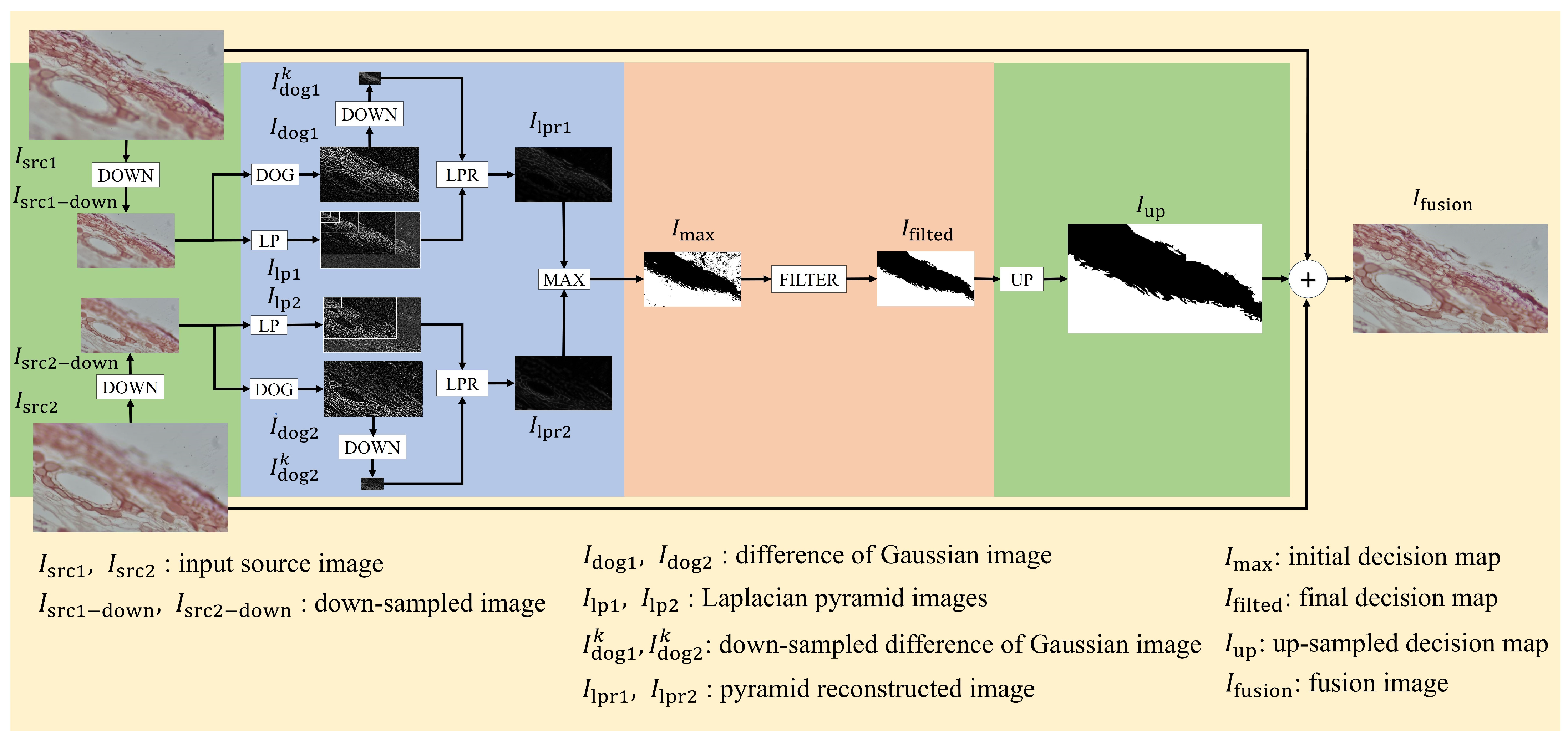
2. Methods
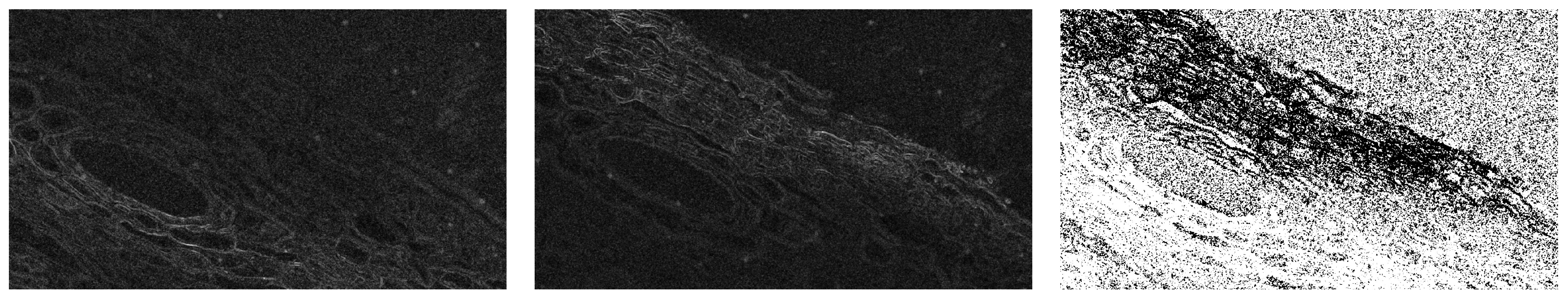
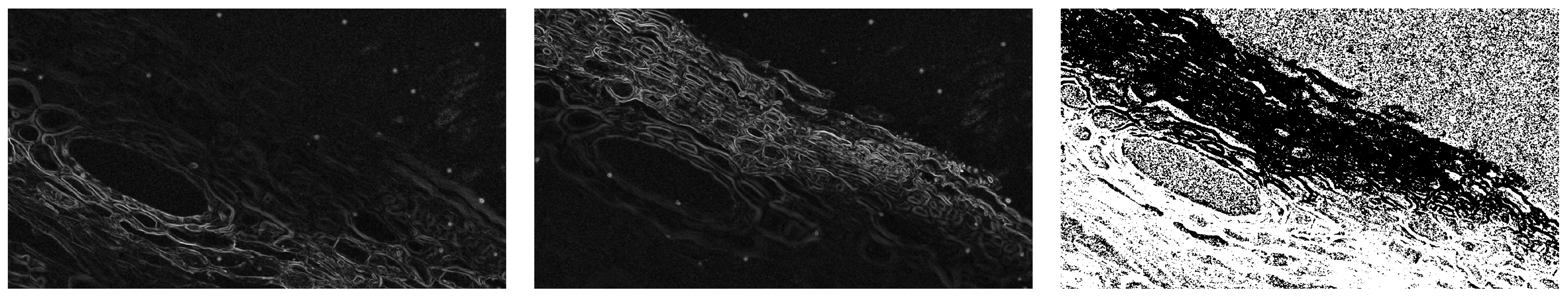
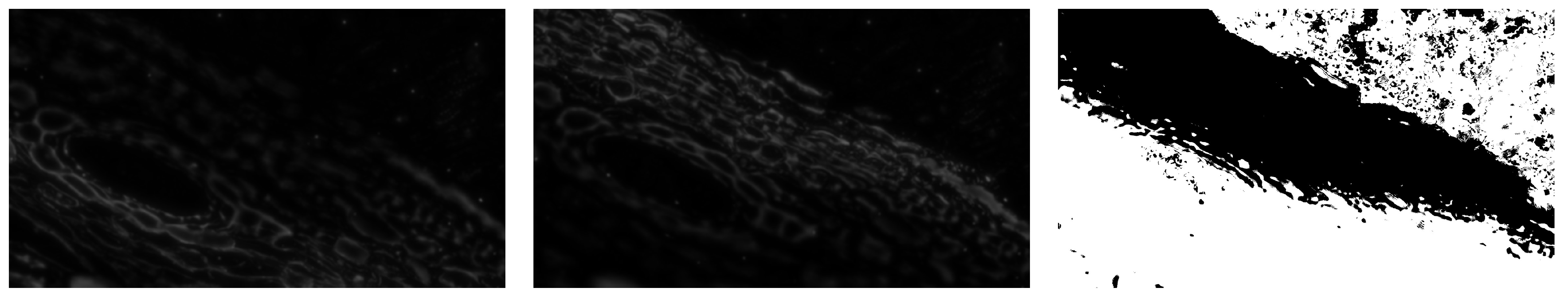
2.1. Focused Region Detection
2.2. Decision Map
2.3. Image Fusion
3. Experimental Results
3.1. Focus Measure
3.2. Quantitative Evaluation
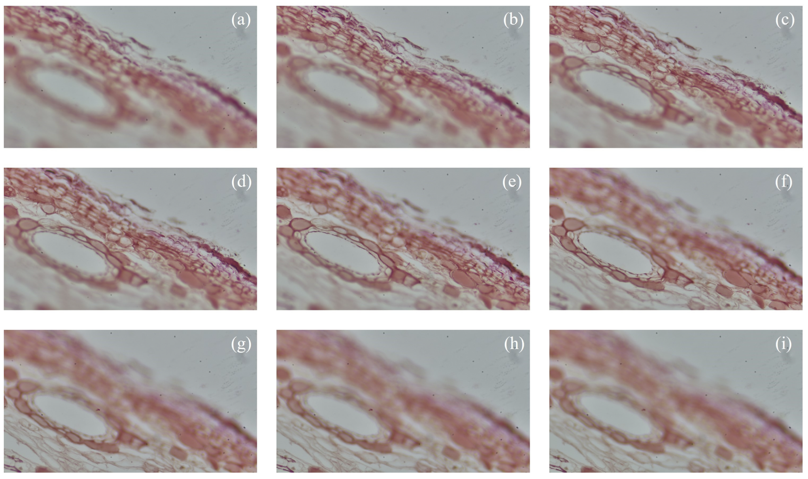
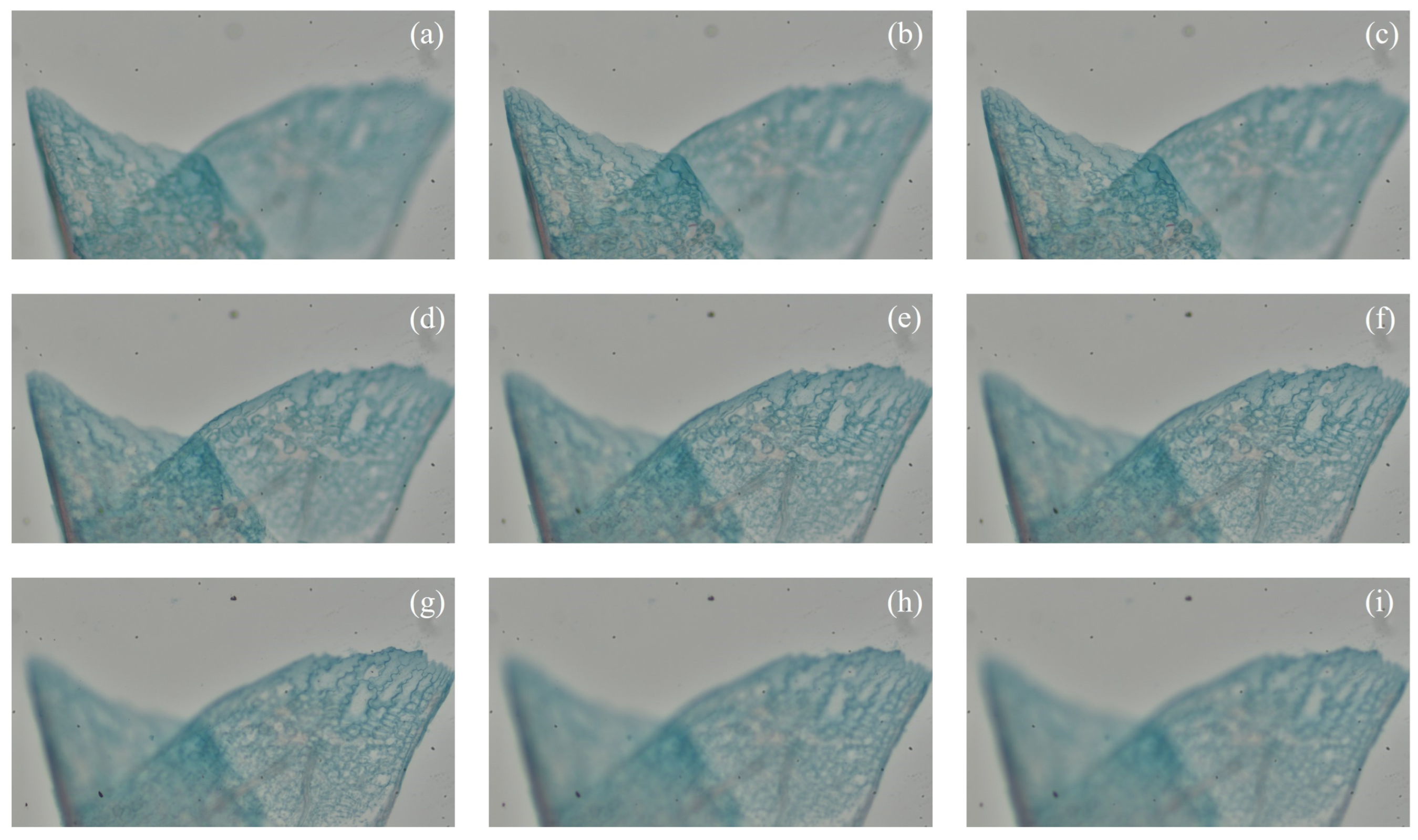
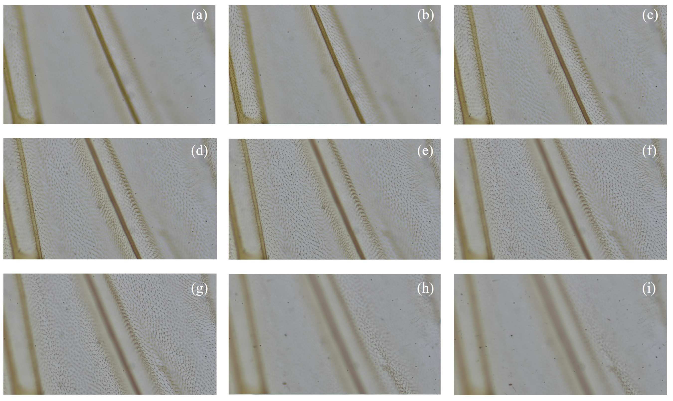
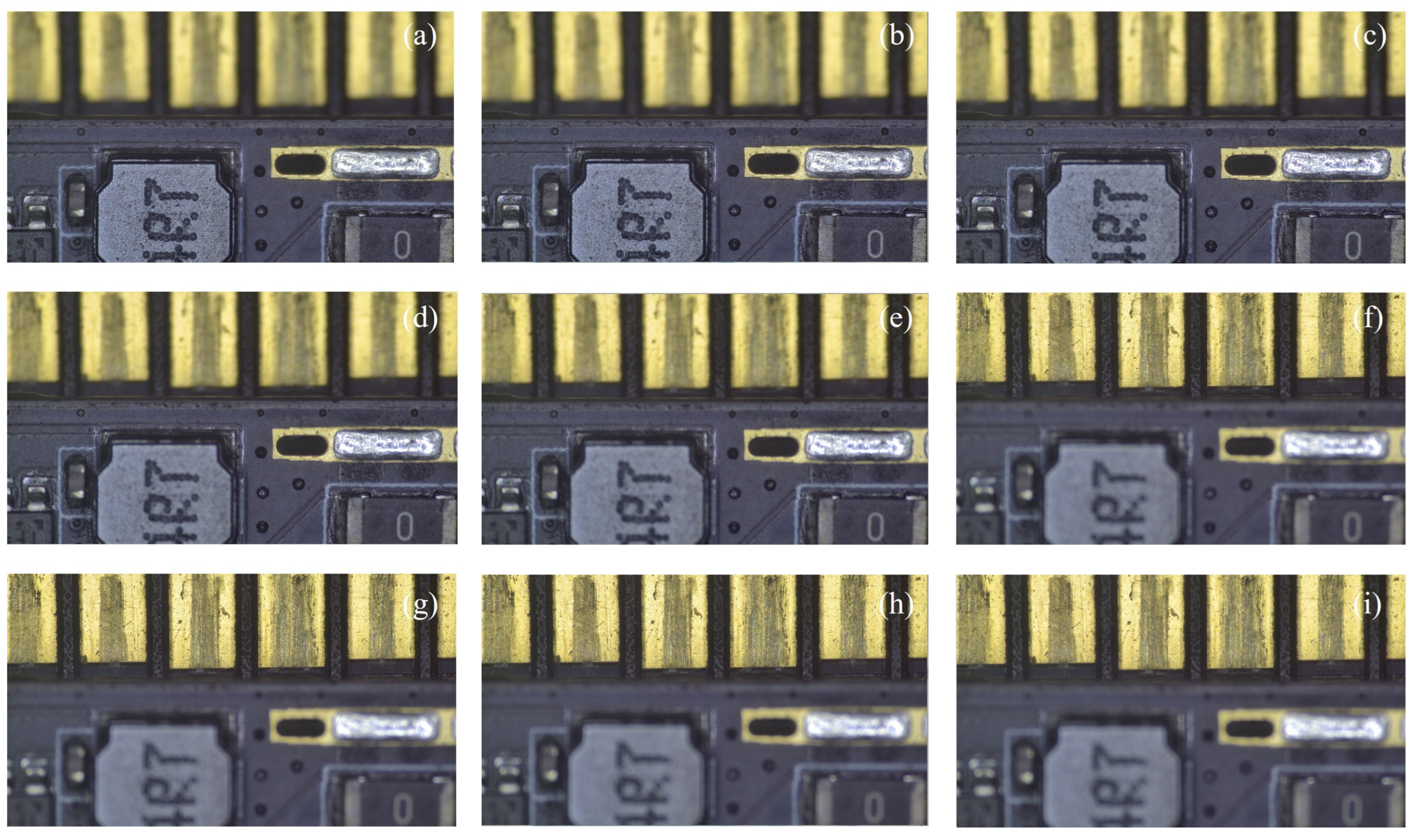
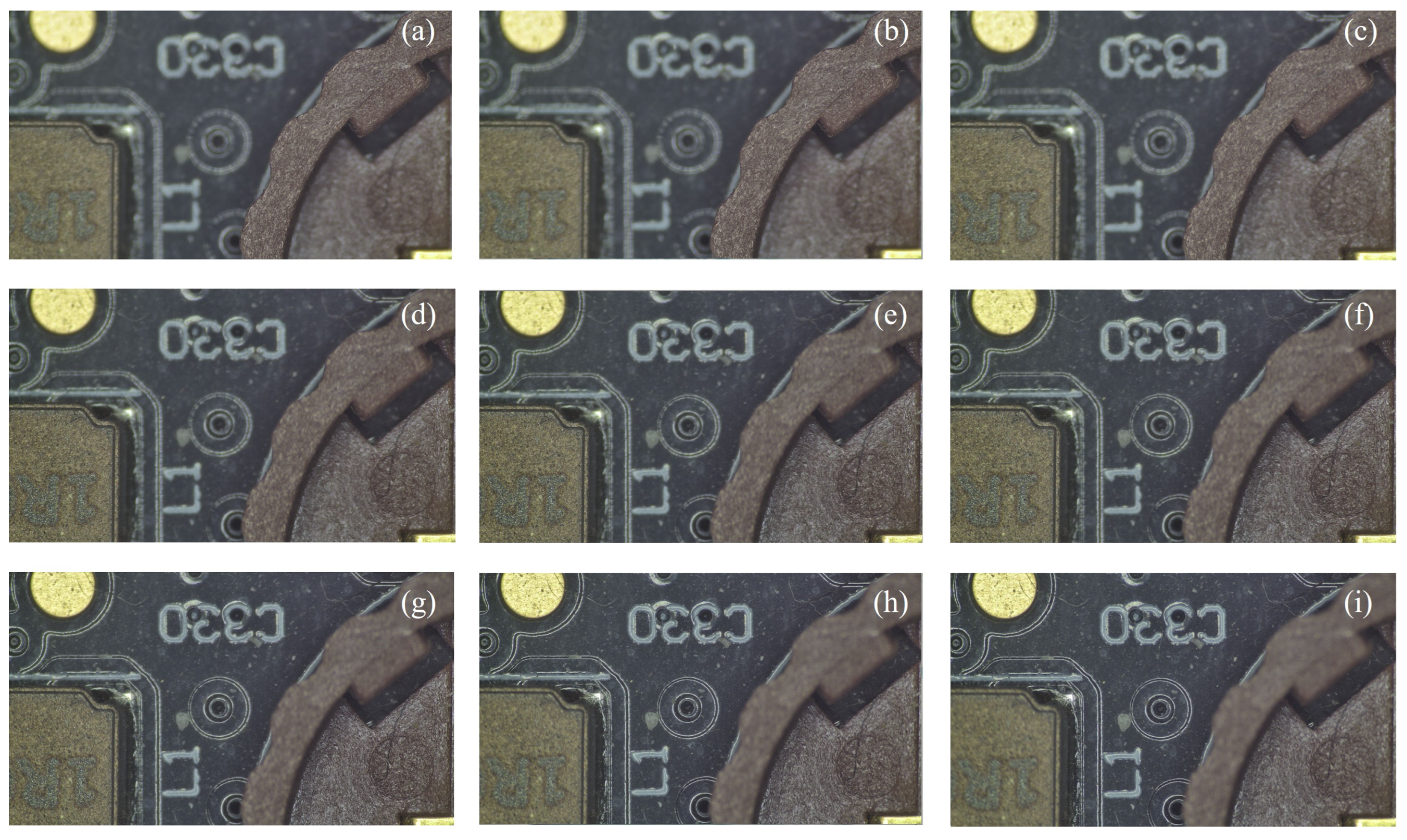
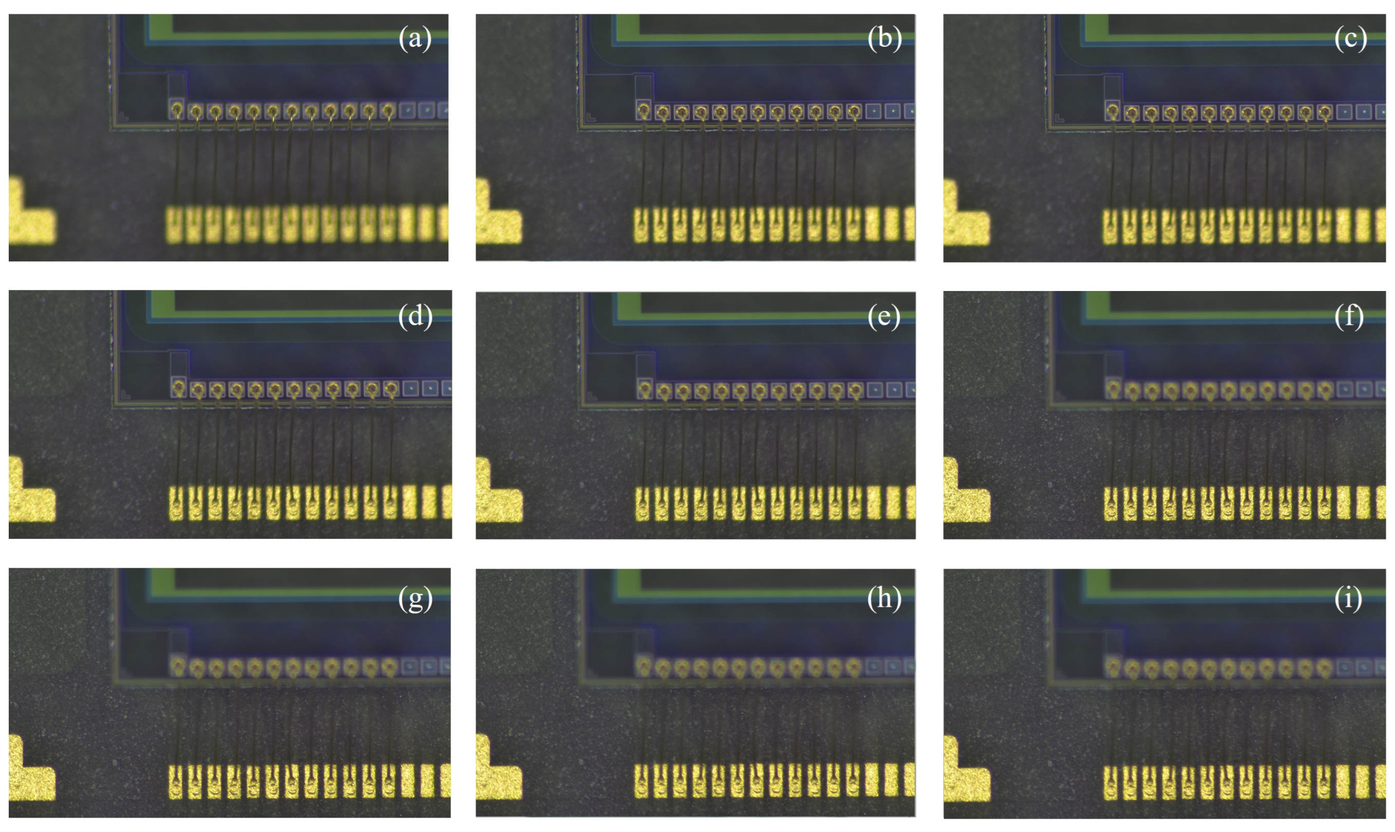
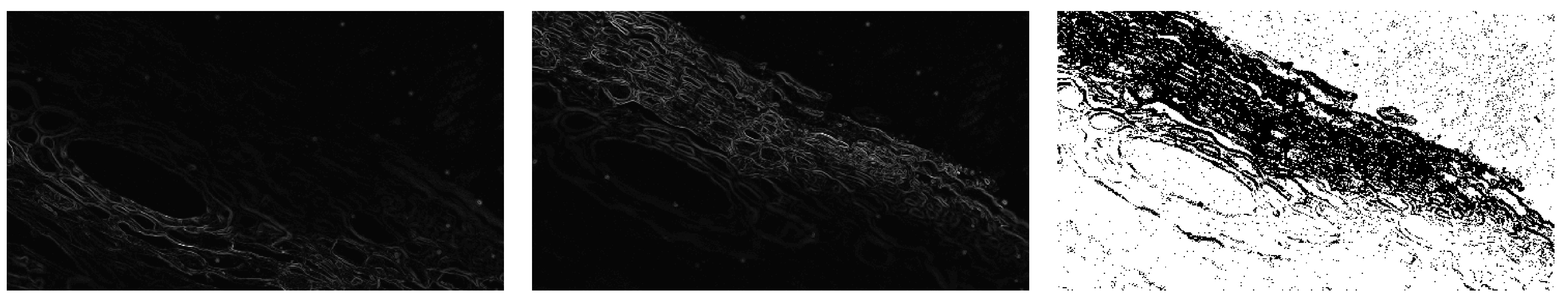
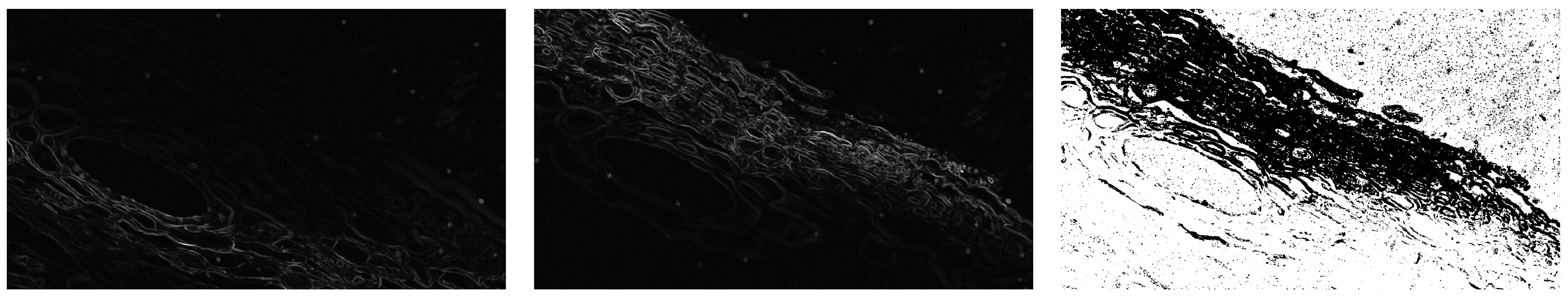
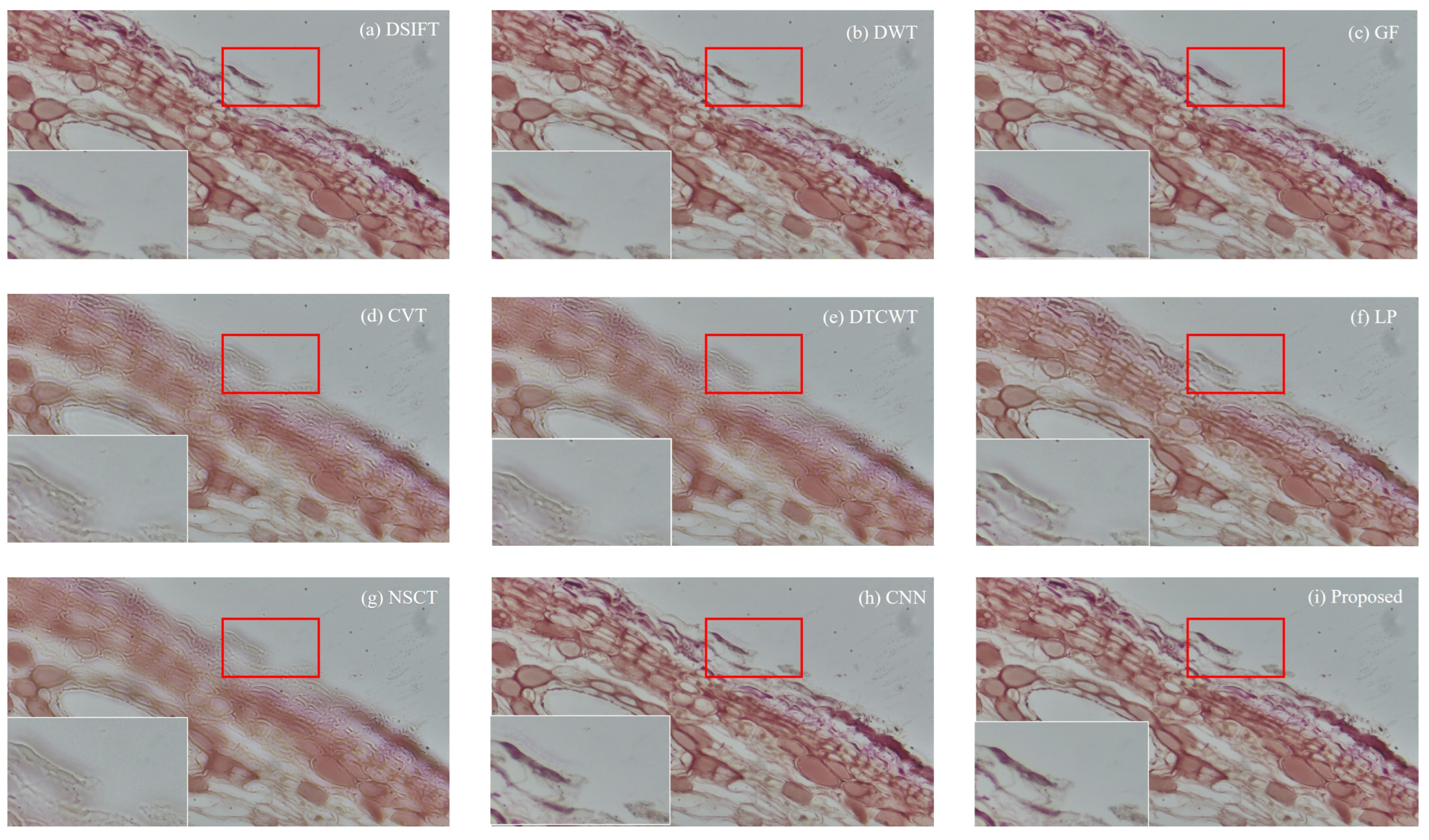
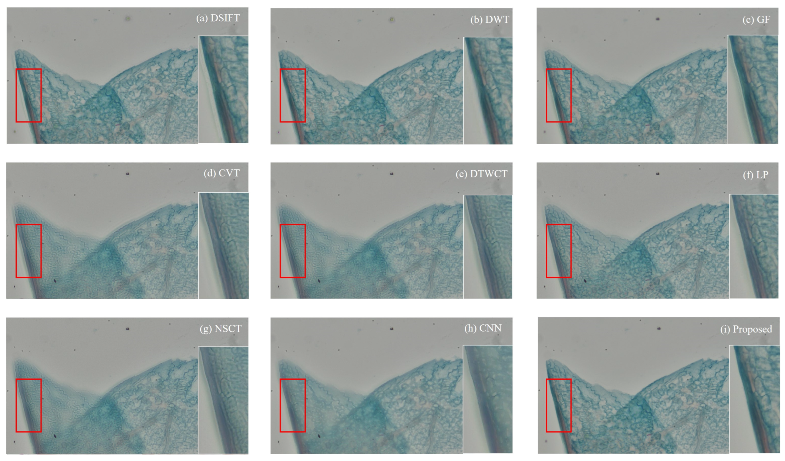
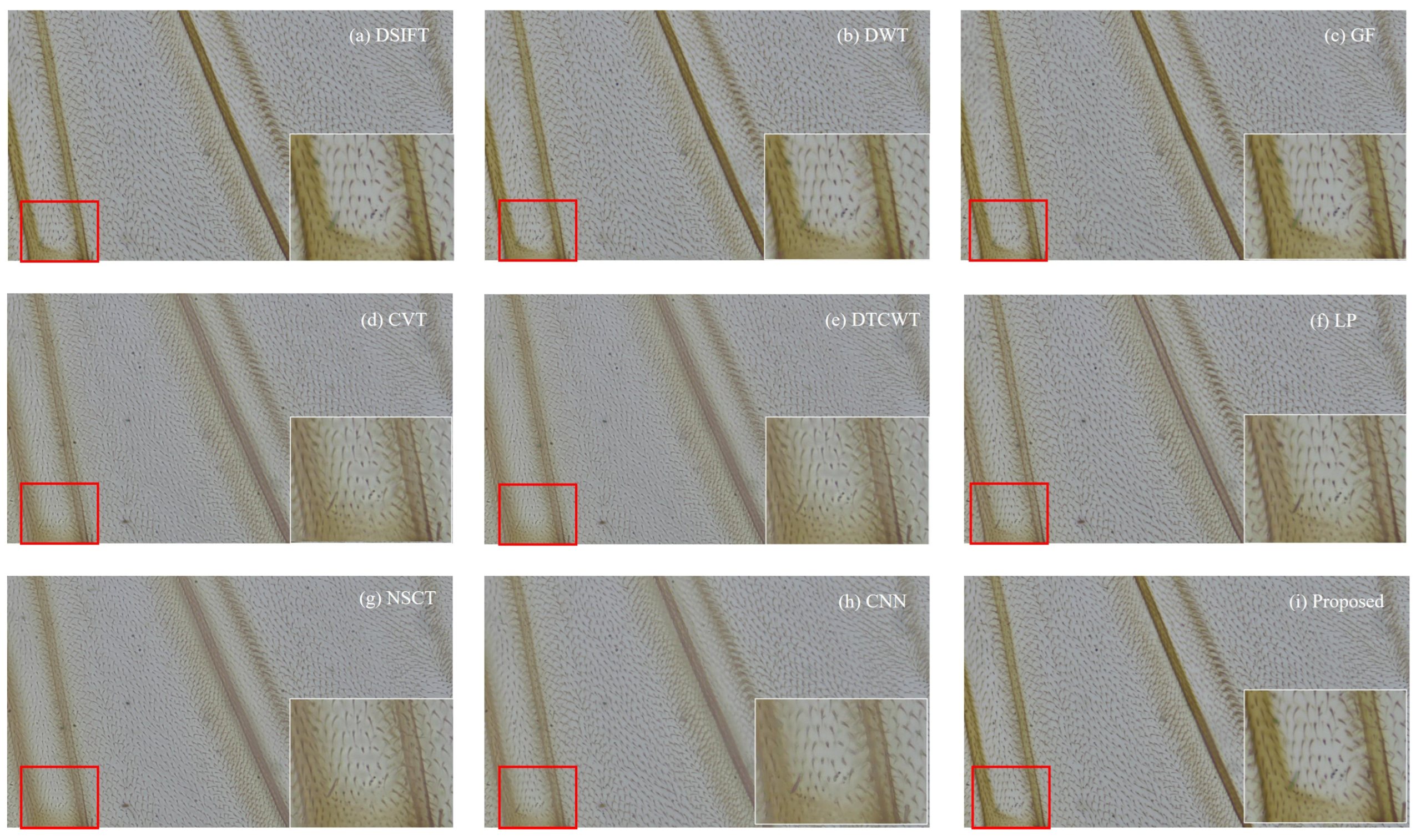
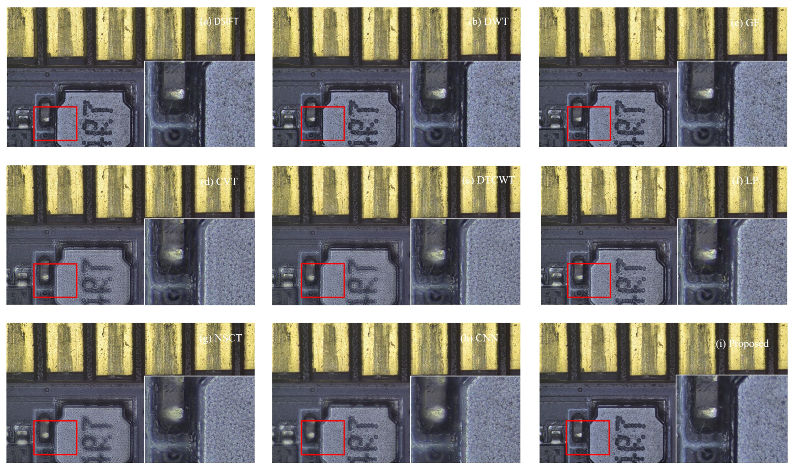
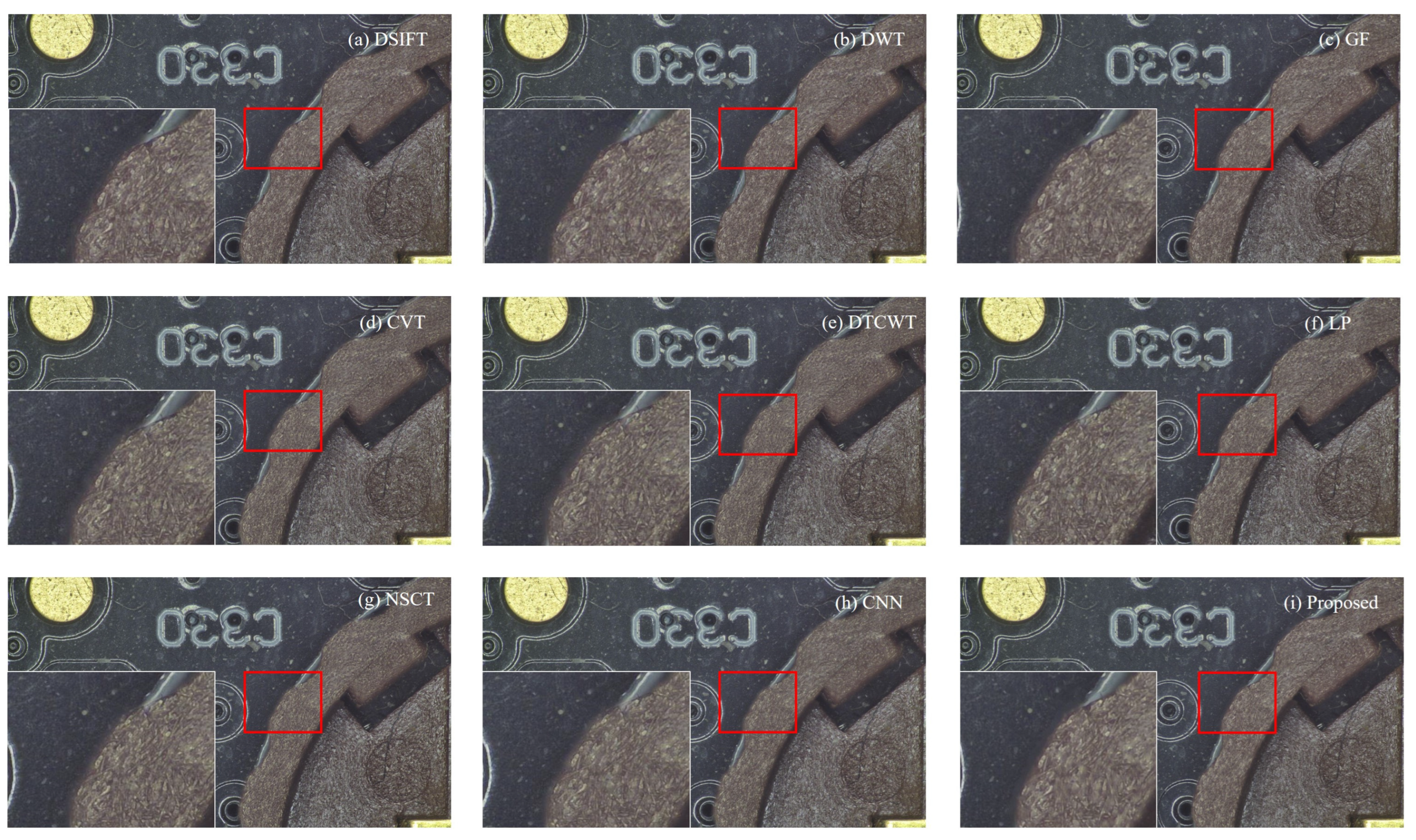
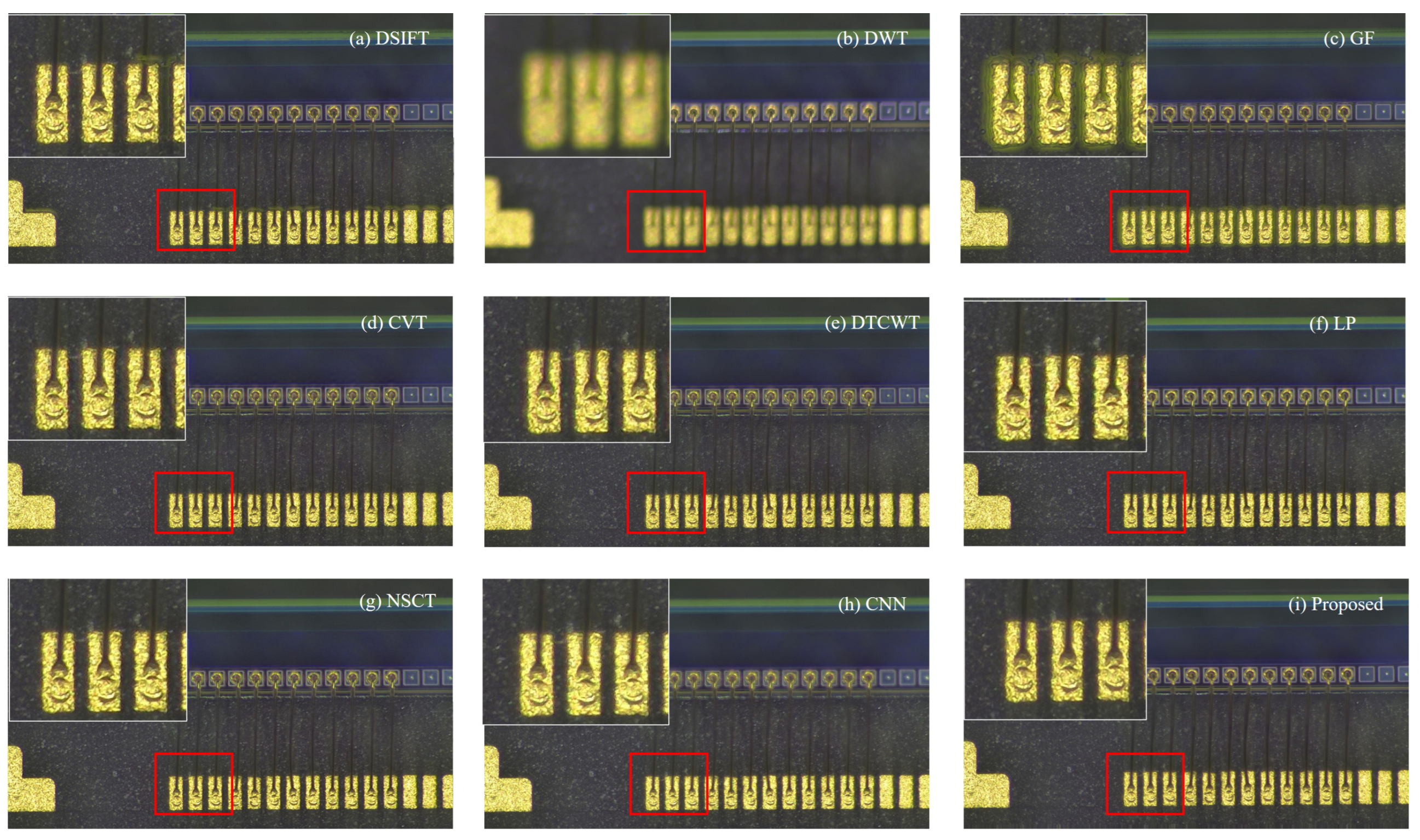
3.2.1. Subjective Visual Comparison
3.2.2. Objective Quantitative Evaluation
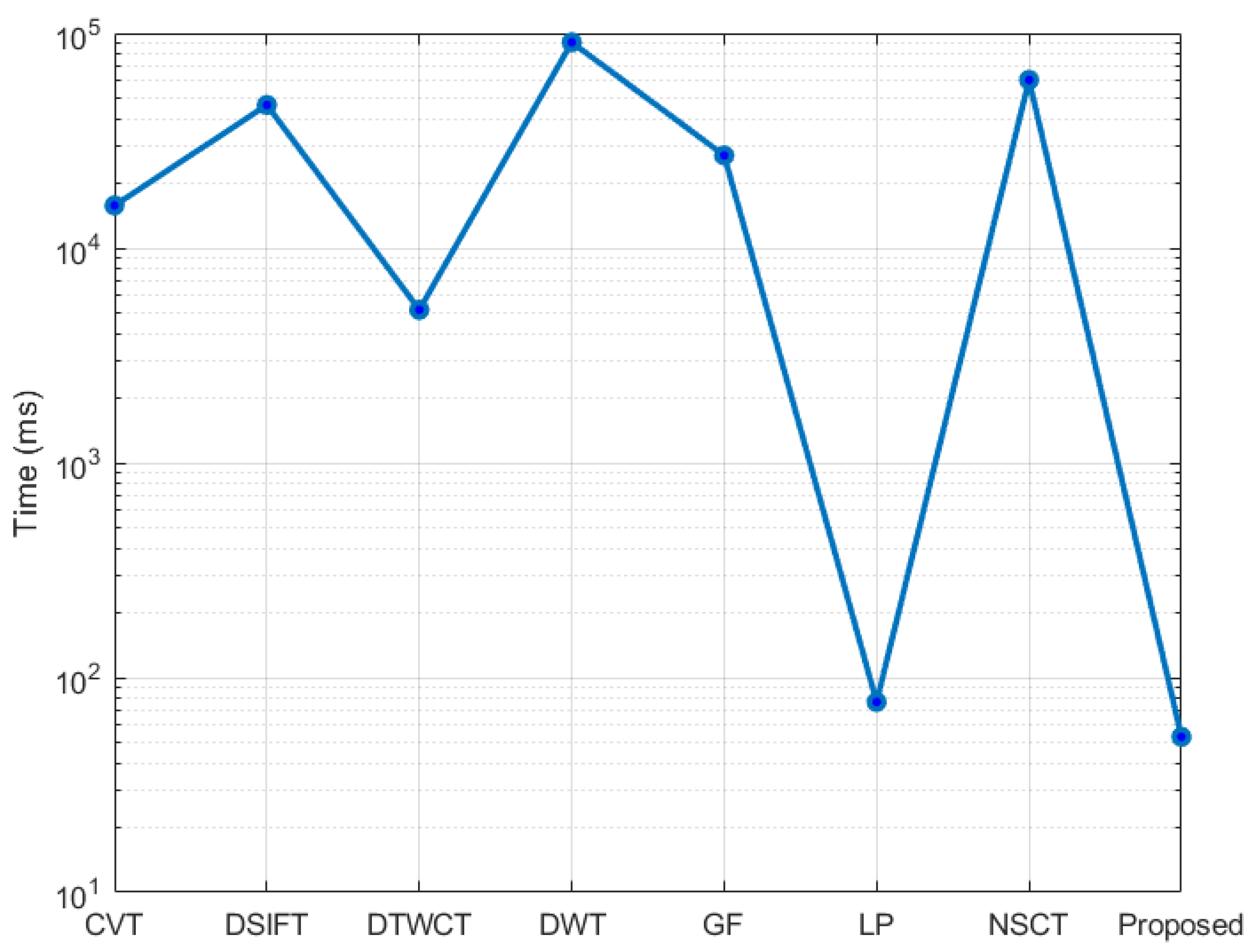
3.3. Computational Efficiency Evaluation
4. Conclusions
Supplementary Materials
Author Contributions
Funding
Institutional Review Board Statement
Informed Consent Statement
Data Availability Statement
Conflicts of Interest
References
- Yuan, T.; Jiang, W.; Ye, Y.Q. Confocal microscopy multi-focus image fusion method based on axial information guidance. Appl. Opt. 2023, 62, 5772–5777. [Google Scholar] [CrossRef] [PubMed]
- Liu, Y.; Wang, L.; Cheng, J. Multi-focus image fusion: A Survey of the state of the art. Inf. Fusion 2020, 64, 71–79. [Google Scholar] [CrossRef]
- Li, X.S.; Zhou, F.Q.; Tan, H.S. Multi-focus image fusion based on nonsubsampled contourlet transform and residual removal. Signal Process. 2021, 184, 108062. [Google Scholar] [CrossRef]
- Chen, J.; Zhang, X.; Peng, X. Shuffle-octave-yolo: A tradeoff object detection method for embedded devices. J. Real-Time Image Process. 2023, 20, 25. [Google Scholar] [CrossRef]
- Hu, Z.H.; Wang, L.; Ding, D.R. An improved multi-focus image fusion algorithm based on multi-scale weighted focus measure. Appl. Intell. 2021, 51, 4453–4469. [Google Scholar] [CrossRef]
- Bai, X.; Liu, M.; Chen, Z.; Wang, P.; Zhang, Y. Multi-focus image fusion through gradient-based decision map construction and mathematical morphology. IEEE Access 2016, 4, 4749–4760. [Google Scholar] [CrossRef]
- Li, S.; Kowk, J.T.; Wang, Y. combination of images with diverse focuses using spatial frequency. Inf. Fusion 2001, 2, 169–176. [Google Scholar] [CrossRef]
- Li, S.T.; Kang, X.D.; Fang, L.Y. Pixel-level image fusion: A survey of the state of the art. Inf. Fusion 2017, 33, 100–112. [Google Scholar] [CrossRef]
- Tian, J.; Liu, G.; Liu, J. Multi-focus image fusion based on edges and focused region extraction. Optik 2018, 171, 611–624. [Google Scholar] [CrossRef]
- Zhang, B.; Lu, X.; Pei, H. Multi-focus image fusion algorithm based on focused region extraction. Neurocomputing 2016, 174, 733–748. [Google Scholar] [CrossRef]
- Yu, M.M.; Zheng, Y.L.; Liao, K.Y. Image quality assessment via spatial-transformed domains multi-feature fusion. IET Image Process. 2022, 14, 648–657. [Google Scholar] [CrossRef]
- Liu, W.; Zheng, Z.; Wang, Z. Robust multi-focus image fusion using lazy random walks with multiscale focus measures. Signal Process. 2021, 179, 107850. [Google Scholar] [CrossRef]
- Hill, P.; Al-Mualla, M.E.; Bull, D. Perceptual Image Fusion Using Wavelets. IEEE Trans. Image Process. 2017, 26, 1076–1088. [Google Scholar] [CrossRef] [PubMed]
- Yang, B.; Li, S. Multi-focus image fusion and restoration with sparse representation. IEEE Trans. Instrum. Meas. 2009, 59, 884–892. [Google Scholar] [CrossRef]
- Yin, H.; Li, Y.; Chai, Y.; Liu, Z.; Zhu, Z. A novel sparse-representation-based multi-focus image fusion approach. Neurocomputing 2016, 216, 216–229. [Google Scholar] [CrossRef]
- Mustafa, H.T.; Yang, J.; Zareapoor, M. Multi-scale convolutional neural network for multi-focus image fusion. Image Vis. Comput. 2019, 85, 26–35. [Google Scholar] [CrossRef]
- Liu, Y.; Chen, X.; Peng, H.; Wang, Z. Multi-focus image fusion with a deep convolutional neural network. Inf. Fusion 2017, 36, 191–207. [Google Scholar] [CrossRef]
- Guo, X.; Nie, R.; Cao, J.; Zhou, D.; Mei, L.; He, K. Fusegan: Learning to fuse multi-focus image via conditional generative adversarial network. IEEE Trans. Multimed. 2019, 21, 1982–1996. [Google Scholar] [CrossRef]
- Li, Y.; Li, X.Y.; Wang, J.Q. Multi-focus image fusion for microscopic depth-of-field extension of waterjet-assisted laser pro-cessing. Int. J. Adv. Manuf. Technol. 2024, 131, 1717–1734. [Google Scholar] [CrossRef]
- Yu, Z.; Bai, X.Z.; Wang, T. Boundary finding based multi-focus image fusion through multi-scale morphological focus-measure. Inf. Fusion 2017, 35, 81–101. [Google Scholar]
- Huang, W.; Jing, Z. Evaluation of focus measures in multi-focus image fusion. Pattern Recognit. Lett. 2007, 28, 493–500. [Google Scholar] [CrossRef]
- Roy, M.; Mukhopadhyay, S. A scheme for edge-based multi-focus Color image fusion. Multimed. Tools Appl. 2020, 79, 24089–24117. [Google Scholar] [CrossRef]
- Pertuz, S.; Puig, D.; Garcia, M.A. Analysis of focus measure operators for shape-from-focus. Pattern Recognit. 2013, 46, 1415–1432. [Google Scholar] [CrossRef]
- Naidu, V.P.S. Multi focus image fusion using the measure of focus. J. Opt. 2012, 41, 117–125. [Google Scholar] [CrossRef]
- Liu, Y.; Liu, S.P.; Wang, Z.F. Multi-focus image fusion with dense SIFT. Inf. Fusion 2015, 23, 139–155. [Google Scholar] [CrossRef]
- Burt, P.; Adelson, E. The Laplacian pyramid as a compact image code. IEEE Trans. Commun 1983, 31, 532–540. [Google Scholar] [CrossRef]
- Nencini, F.; Garzelli, A.; Baronti, S.; Alparone, L. Remote sensing image fusion using the curvelet transform. Inf. Fusion 2007, 8, 143–156. [Google Scholar] [CrossRef]
- Lewis, J.; O’Callaghan, R.; Nikolov, S.; Bull, D.; Canagarajah, N. Pixel and regionbased image fusion with complex wavelets. Inf. Fusion 2007, 8, 119130. [Google Scholar] [CrossRef]
- Zhang, Q.; Guo, B. Multifocus image fusion using the nonsubsampled contourlet transform. Signal Process. 2009, 89, 1334–1346. [Google Scholar] [CrossRef]
- Liu, Y.; Wang, Z.F. Multi-focus image fusion based on wavelet transform and adaptive block. J. Image Graph. 2013, 18, 1435–1444. [Google Scholar]
- Qiu, X.; Li, M.; Zhang, L.; Yuan, X. Guided filter-based multi-focus image fusion through focus region detection. Signal Process. Image Commun. 2019, 72, 35–46. [Google Scholar] [CrossRef]
- Zhang, Q.; Maldague, X. An adaptive fusion approach for infrared and visible images based on NSCT and compressed sensing. Infrared Phys. Technol. 2016, 74, 11–20. [Google Scholar] [CrossRef]
- Wang, Z.Y.; Zhuang, J.J.; Ye, S.C. Image Restoration Quality Assessment Based on Regional Differential Information Entropy. Entropy 2023, 25, 144. [Google Scholar] [CrossRef] [PubMed]
- Cheng, G.Q.; Huang, J.C.; Liu, Z. Image quality assessment using natural image statistics in gradient domain. AEU-Int. J. Electron. Commun. 2011, 65, 392–397. [Google Scholar] [CrossRef]
- Wang, Z.; Bovik, A.C.; Sheikh, H.R.; Simoncelli, E.P. Image quality assessment: From error visibility to structural similarity. IEEE Trans. Image Process. 2004, 13, 600–612. [Google Scholar] [CrossRef]
- Liu, Z.; Blasch, E.; Xue, Z. Objective Assessment of Multiresolution Image Fusion Algorithms for Context Enhancement in Night Vision: A Comparative Study. IEEE Trans. Pattern Anal. Mach. Intell. 2012, 34, 94–109. [Google Scholar] [CrossRef]


| Gray Level Variance | Energy of Gradient | Energy of Laplacian | Spatial Frequency | Proposed | |
|---|---|---|---|---|---|
| Time (ms) | 6.2 | 19.6 | 20.5 | 96.7 | 30.4 |
| AG | STD | IE | SSIM | ||
|---|---|---|---|---|---|
| CVT [27] | 19.3246 | 27.3442 | 6.07645 | 0.847888 | 0.810852 |
| DSIFT [25] | 20.7745 | 29.5445 | 6.22825 | 0.877708 | 0.815088 |
| DTCWT [28] | 18.3885 | 27.221 | 6.03925 | 0.85066 | 0.811746 |
| DWT [30] | 20.0187 | 30.5857 | 6.24273 | 0.88202 | 0.815357 |
| GF [31] | 20.187 | 29.7431 | 6.1772 | 0.87898 | 0.814651 |
| LP [26] | 20.7483 | 28.8912 | 6.14031 | 0.868556 | 0.811973 |
| NSCT [29] | 18.3428 | 27.2727 | 6.05721 | 0.856632 | 0.81205 |
| CNN [17] | 17.3523 | 27.1024 | 6.08908 | 0.876586 | 0.81058 |
| Proposed | 20.3064 | 29.8402 | 6.25856 | 0.882812 | 0.815447 |
| Proposed * | 20.3165 | 29.9202 | 6.25086 | 0.872812 | 0.82517 |
| CVT [27] | 12.3632 | 10.7028 | 5.54002 | 0.909865 | 0.81881 |
| DSIFT [25] | 12.4924 | 12.0779 | 5.54811 | 0.919278 | 0.823326 |
| DTCWT [28] | 11.5306 | 10.6387 | 5.49342 | 0.912781 | 0.819688 |
| DWT [30] | 11.9218 | 12.0684 | 5.5686 | 0.921628 | 0.823993 |
| GF [31] | 11.9296 | 11.6672 | 5.52452 | 0.922296 | 0.822911 |
| LP [26] | 13.3136 | 11.2697 | 5.58323 | 0.912336 | 0.820555 |
| NSCT [29] | 12.4523 | 10.6912 | 5.55654 | 0.910408 | 0.819554 |
| CNN [17] | 10.4320 | 10.3358 | 5.5252 | 0.91216 | 0.82354 |
| Proposed | 12.951 | 11.9026 | 5.64674 | 0.924828 | 0.824449 |
| Proposed * | 12.936 | 11.8209 | 5.68476 | 0.926329 | 0.823215 |
| CVT [27] | 31.9613 | 18.9883 | 5.61926 | 0.793585 | 0.804661 |
| DSIFT [25] | 32.2706 | 24.6258 | 5.6433 | 0.804718 | 0.806639 |
| DTCWT [28] | 31.3471 | 18.5883 | 5.54529 | 0.797095 | 0.804772 |
| DWT [30] | 30.4422 | 24.8534 | 5.64766 | 0.816291 | 0.806505 |
| GF [31] | 31.0241 | 24.0161 | 5.64718 | 0.819189 | 0.806654 |
| LP [26] | 33.4949 | 20.8382 | 5.60456 | 0.799082 | 0.805762 |
| NSCT [29] | 31.4199 | 18.7381 | 5.50142 | 0.807033 | 0.815033 |
| CNN [17] | 30.5334 | 18.3291 | 5.43541 | 0.843392 | 0.816261 |
| Proposed | 31.1584 | 24.3391 | 5.6408 | 0.82323 | 0.806973 |
| Proposed * | 31.1687 | 24.4215 | 5.6132 | 0.84312 | 0.809014 |
| CVT [27] | 59.5814 | 38.3868 | 7.43451 | 0.871984 | 0.815922 |
| DSIFT [25] | 62.0276 | 39.2977 | 7.44373 | 0.911055 | 0.817409 |
| DTCWT [28] | 58.6648 | 38.1909 | 7.43234 | 0.881985 | 0.816391 |
| DWT [30] | 58.9759 | 39.2304 | 7.43481 | 0.901077 | 0.817677 |
| GF [31] | 59.0821 | 39.2826 | 7.43744 | 0.920131 | 0.818055 |
| LP [26] | 61.1618 | 39.4982 | 7.46599 | 0.893253 | 0.8161 |
| NSCT [29] | 58.4832 | 38.2411 | 7.43975 | 0.899051 | 0.816003 |
| CNN [17] | 58.258 | 37.2785 | 7.4391 | 0.89589 | 0.81758 |
| Proposed | 61.4661 | 38.9481 | 7.44318 | 0.928969 | 0.818154 |
| Proposed * | 61.5316 | 38.8146 | 7.42153 | 0.929614 | 0.818562 |
| CVT [27] | 53.0906 | 28.6474 | 6.80511 | 0.858056 | 0.819864 |
| DSIFT [25] | 53.5911 | 28.2358 | 6.77732 | 0.866079 | 0.81903 |
| DTCWT [28] | 52.4223 | 28.441 | 6.79821 | 0.862685 | 0.820285 |
| DWT [30] | 51.3696 | 28.1972 | 6.77436 | 0.870141 | 0.82007 |
| GF [31] | 51.4012 | 28.1351 | 6.77095 | 0.872878 | 0.820718 |
| LP [26] | 53.109 | 29.375 | 6.83198 | 0.867835 | 0.819624 |
| NSCT [29] | 53.008 | 29.0032 | 6.81995 | 0.865614 | 0.82048 |
| CNN [17] | 49.8133 | 28.8426 | 6.75652 | 0.863738 | 0.812352 |
| Proposed | 49.4289 | 28.8073 | 6.84009 | 0.866481 | 0.821801 |
| Proposed * | 49.4128 | 28.7056 | 6.85168 | 0.867186 | 0.821704 |
| CVT [27] | 32.5517 | 16.5784 | 5.95006 | 0.91023 | 0.815478 |
| DSIFT [25] | 33.1308 | 17.065 | 5.93774 | 0.89124 | 0.820368 |
| DTCWT [28] | 31.6427 | 16.2941 | 5.93283 | 0.917782 | 0.816438 |
| DWT [30] | 30.3168 | 16.7354 | 6.02287 | 0.762649 | 0.815396 |
| GF [31] | 26.2456 | 17.1092 | 6.06482 | 0.874978 | 0.80518 |
| LP [26] | 33.7763 | 17.6949 | 5.99203 | 0.921932 | 0.816358 |
| NSCT [29] | 32.7835 | 16.8062 | 5.94666 | 0.92872 | 0.816188 |
| CNN [17] | 31.6019 | 16.8886 | 6.00345 | 0.818782 | 0.818782 |
| Proposed | 32.0278 | 17.7999 | 5.88154 | 0.924163 | 0.827311 |
| Proposed * | 32.0652 | 17.8013 | 5.87165 | 0.925105 | 0.828196 |
| CVT [27] | 34.8121 | 23.4413 | 6.2375 | 0.8652 | 0.81426 |
| DSIFT [25] | 35.7145 | 25.1411 | 6.2630 | 0.8783 | 0.81697 |
| DTCWT [28] | 33.9993 | 23.229 | 6.2068 | 0.8704 | 0.81488 |
| DWT [30] | 33.8408 | 25.2784 | 6.2818 | 0.8589 | 0.81649 |
| GF [31] | 33.3116 | 24.9922 | 6.2703 | 0.8814 | 0.81469 |
| LP [26] | 35.9339 | 24.5945 | 6.2696 | 0.8771 | 0.81506 |
| NSCT [29] | 34.4149 | 23.4587 | 6.2202 | 0.8779 | 0.81655 |
| CNN [17] | 32.9984 | 23.1295 | 6.2081 | 0.8684 | 0.81651 |
| Proposed | 34.5564 | 25.2728 | 6.2851 | 0.8917 | 0.81902 |
| Proposed * | 34.5718 | 25.2473 | 6.2822 | 0.8940 | 0.82097 |
| LP [26] | Proposed | |
|---|---|---|
| Time | 9916 ms | 586 ms |
Disclaimer/Publisher’s Note: The statements, opinions and data contained in all publications are solely those of the individual author(s) and contributor(s) and not of MDPI and/or the editor(s). MDPI and/or the editor(s) disclaim responsibility for any injury to people or property resulting from any ideas, methods, instructions or products referred to in the content. |
© 2025 by the authors. Licensee MDPI, Basel, Switzerland. This article is an open access article distributed under the terms and conditions of the Creative Commons Attribution (CC BY) license (https://creativecommons.org/licenses/by/4.0/).
Share and Cite
Chen, H.; Du, X.; Huang, H.; Zhao, T. A Real-Time High-Resolution Multi-Focus Image Fusion Algorithm Based on Multi-Scale Feature Aggregation. Appl. Sci. 2025, 15, 6967. https://doi.org/10.3390/app15136967
Chen H, Du X, Huang H, Zhao T. A Real-Time High-Resolution Multi-Focus Image Fusion Algorithm Based on Multi-Scale Feature Aggregation. Applied Sciences. 2025; 15(13):6967. https://doi.org/10.3390/app15136967
Chicago/Turabian StyleChen, Huawei, Xingkai Du, Hongchuan Huang, and Tingyu Zhao. 2025. "A Real-Time High-Resolution Multi-Focus Image Fusion Algorithm Based on Multi-Scale Feature Aggregation" Applied Sciences 15, no. 13: 6967. https://doi.org/10.3390/app15136967
APA StyleChen, H., Du, X., Huang, H., & Zhao, T. (2025). A Real-Time High-Resolution Multi-Focus Image Fusion Algorithm Based on Multi-Scale Feature Aggregation. Applied Sciences, 15(13), 6967. https://doi.org/10.3390/app15136967