Article

Smooth Optimised A*-Guided DWA for Mobile Robot Path Planning

School of Engineering, Shanghai Ocean University, Shanghai 201306, China
*
Author to whom correspondence should be addressed.
Appl. Sci. 2025, 15(13), 6956; https://doi.org/10.3390/app15136956
Submission received: 19 May 2025 / Revised: 13 June 2025 / Accepted: 15 June 2025 / Published: 20 June 2025

Abstract

In mobile robot path planning, the traditional A* algorithm suffers from high path redundancy and poor smoothness, while the Dynamic Window Approach (DWA) tends to deviate from the global optimal path and has low efficiency in avoiding dynamic obstacles when integrated with global path planning. To address these issues, a smoothing optimised A*-guided DWA fusion algorithm (SOA-DWA) is proposed in this paper. Firstly, the A* algorithm was improved by introducing a path smoothing strategy and path pruning mechanism, generating a globally optimal path that complied with the vehicle kinematic constraints. Secondly, three sub-functions were introduced into the evaluation function of the DWA algorithm: the distance evaluation between the reference trajectory and the global path, the path direction evaluation, and the dynamic obstacle avoidance evaluation, to enhance the real-time performance of dynamic obstacle avoidance and the consistency of the global path. The SOA-DWA algorithm ensured that the mobile robot could effectively avoid obstacles in complex environments without deviating from the global optimal path. Thirdly, experimental results show that in a static environment, the path length and turning angle of the SOA-DWA algorithm are reduced by an average of 13.3% and 16.25%, respectively, compared with the traditional algorithm. In a dynamic environment, the path length and turning angle are reduced by an average of 10.5% and 14.5% compared to the traditional DWA algorithm, respectively, significantly improving the smoothness of the path and driving safety. Compared to the existing fusion algorithm, the SOA-DWA algorithm reduces the path length by an average of 10.1%, improves planning efficiency by an average of 42%, and effectively enhances obstacle avoidance efficiency. Finally, the effectiveness of the improved algorithm proposed in this paper was further verified by mobile robot experiments.

1. Introduction

A mobile robot is an autonomous system that performs locomotion using onboard power (e.g., batteries) and integrates perception sensors (e.g., lidar, stereo cameras) with navigation algorithms [1,2]. Under the control of the guidance system, it completes path planning and trajectory tracking control [3]. The specific steps of path planning include determining the starting point and target point; planning a reasonable driving route from the starting point to the target point; using an obstacle avoidance algorithm to ensure that there is no collision with obstacles during driving, while the optimal path is determined based on predefined optimisation objectives, such as minimising distance, energy consumption, or travel time [4,5]. This process not only requires considering the geometry of the path, but also needs to comprehensively evaluate multiple factors such as operating efficiency and energy consumption to achieve efficient, safe and environmentally friendly transportation of mobile robots [6,7]. At present, in the research on mobile robot path planning, scholars have proposed clear technical routes for different scenario requirements. In terms of global path planning, the research focuses on classic algorithms such as the A* Algorithm [8,9], the Dijkstra Algorithm [10], and the RRT Algorithm [11,12], and further improves them by introducing intelligent algorithms such as machine learning [13] and deep reinforcement learning [14]. In terms of local path planning, the focus is mainly on the Dynamic Window Algorithm (DWA) [15], Ant Colony Algorithm [16], and Taboo Search Algorithm [17], which have shown superior performance in dynamic obstacle avoidance, real-time trajectory optimisation, etc. It is worth noting that in recent years, the trend of integrated application of the two types of algorithms has become increasingly obvious, and the overall planning effect can be improved by complementing each other’s advantages.
Scholars have conducted extensive research on the A* algorithm and its improved algorithm in the field of mobile robots, achieving remarkable results. The authors of [18] significantly enhanced the efficiency of 3D path planning by optimising the heuristic function of the A* algorithm, introducing a turning penalty strategy, and implementing search domain priority allocation. This approach effectively reduced computational load and search costs. The authors of [19] significantly enhanced path planning efficiency, reduced path cost, and improved trajectory smoothness through the implementation of limited jump point search and path optimisation strategies. The authors of [20] enhanced the path planning performance by implementing a dynamically weighted heuristic function and path corner reduction strategy, which improved search efficiency and minimised global path turns. The authors of [21] generated smoother and optimised paths by introducing heuristic functions with variable weights, penalties and fifth-order Bessel curves and optimising the paths by combining with the ant colony algorithm. The authors of [22] optimised the paths by adjusting the neighborhood search strategy, introducing dynamic weighting heuristic function and key node extraction strategy, which reduces the search time and redundant nodes, and optimises the efficiency of path planning. The authors of [8] proposed an improved approach by replacing the octal neighborhood with obstacle-free rectangular boundaries and incorporating bidirectional search with Euclidean distance estimation, which effectively reduced redundant nodes and search time. Furthermore, the algorithm introduced an adaptive cost function to enhance road safety and employed the Slide-Rail method to optimise path smoothness. However, a fundamental limitation persists, as conventional A*-based algorithms, including most improved versions, cannot accommodate dynamic obstacles, consequently producing non-executable paths in dynamically changing environments.
The Dynamic Window Approach (DWA) specializes in local dynamic obstacle avoidance, demonstrating robust capability in handling real-time environmental changes. The authors of [23] significantly improved path planning efficiency and safety for service robots in dense crowds through several key innovations: pedestrian and crowd interaction space modeling, dynamic pedestrian azimuth constraints, classification-based decision making, and adaptive velocity weighting adjustment. Compared to conventional DWA, their social-DWA achieves superior performance in pedestrian/group avoidance, motion velocity optimisation, and travel time reduction while maintaining effective safety distances, thereby enhancing overall path planning flexibility and adaptability. However, the improved algorithm may encounter elevated computational complexity in high-density environments, particularly when processing multiple dynamic obstacles, which could increase system computational load. The authors of [15] proposed an enhanced DWA to address the inherent limitation of fixed parameters in balancing safety and speed in complex environments. By refining the velocity cost function and incorporating a target-point distance cost function, their approach improves path smoothness and inspection robots’ navigation capability. While the modified algorithm demonstrates significantly better obstacle avoidance performance in complex settings, it introduces higher computational demands, necessitating further optimisation of the fuzzy control module to enhance real-time performance. A fundamental limitation persists, as locally planned paths may deviate from global optima, and the obstacle avoidance efficiency remains inadequate for complex scenarios with numerous dynamic obstacles.
In summary, path planning for mobile robots faces several persistent challenges: the traditional A* algorithm often produces paths with high redundancy and poor smoothness; integrating the DWA with global planners can cause the robot to deviate from the optimal path; and the efficiency of dynamic obstacle avoidance remains limited. To overcome these issues, this paper presents a Smooth-Optimised A*-Guided DWA (SOA-DWA) algorithm. The proposed solution implements two key innovations. First, it implements an enhanced A* algorithm incorporating path smoothing and redundant node elimination to generate kinematically feasible global optimum paths. Second, the DWA evaluation function is enhanced by incorporating three subcomponents: a trajectory distance metric to the global path, an evaluation of directional alignment, and a dynamic obstacle avoidance metric. These additions significantly improve both real-time obstacle avoidance and adherence to the global path. Comprehensive simulation experiments on simple and complex 2D grid maps as well as on real-world scenarios demonstrate the effectiveness of the algorithm in different operational scenarios.
The main contributions and uniqueness of this study include the following four areas. (1) A path pruning strategy and path smoothing strategy are added to the traditional A* algorithm to optimise the search path and reduce the number of redundant nodes and turns. (2) A global path constraint strategy is proposed to solve the problem of deviating from the global optimal path when the DWA algorithm incorporates the global path planning algorithm. (3) An obstacle avoidance efficiency optimisation strategy is proposed to improve the efficiency when avoiding obstacles. (4) A fusion algorithm for smooth optimisation of A*-guided DWA is proposed, which makes the mobile robot return to the global optimal path more efficiently while ensuring safe obstacle avoidance.
The remainder of this paper is organised as follows. The improved A* algorithm is presented in Section 2. Section 3 presents the improved DWA algorithm. Section 4 presents the fusion algorithm for smooth optimised A*-guided DWA. Section 5 analyzes the performance of the fusion algorithm. Section 6 summarizes the paper.

2. Global Path Planning

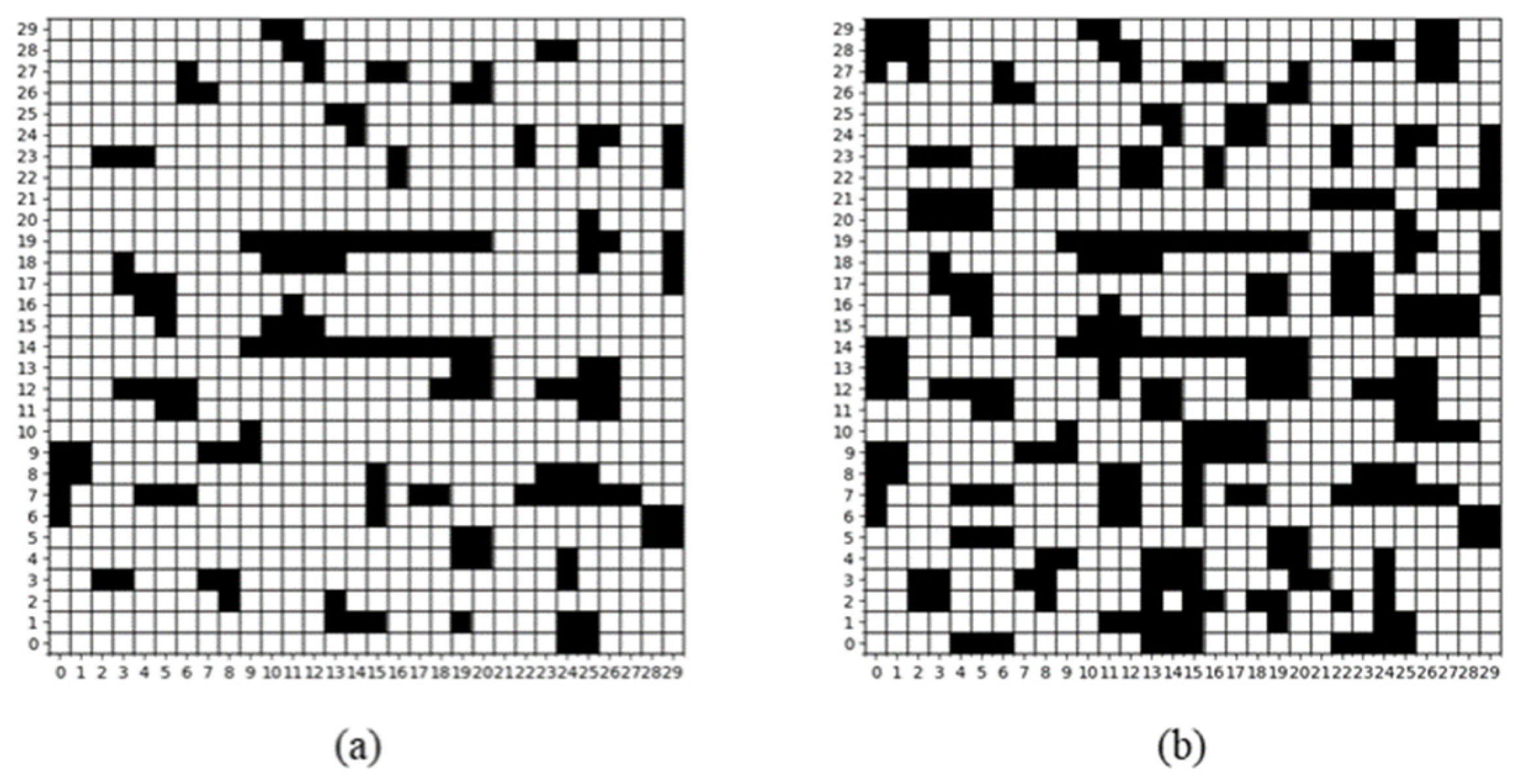
2.1. Environment Building

As shown in Figure 1a,b depict a 30 × 30 simple environment with 19.8% obstacle coverage and a 30 × 30 complex environment with 24.3% obstacle coverage, respectively. In raster maps, each cell represents 1 m × 1 m in the actual physical space. The grid-based representation uses black cells to denote impassable obstacle regions, while white cells indicate navigable areas for robot movement.

2.2. Traditional A* Algorithm

Mobile robots need to plan a path from the starting point to the target point within limited time, and consider factors such as the distance and traffic conditions. Thus, selecting an efficient algorithm that ensures high-quality paths is critical. The A* algorithm can comprehensively consider the actual cost from the starting point to the current node and the estimated cost from the current node to the target node. By minimising the total cost at each node, A* identifies the optimal search path and efficiently computes the shortest path within a constrained search space. The total cost of the node is as shown in Equation (1).
f n = g n + h n
The heuristic function value h n has a significant impact on the performance of the A* algorithm. If h n is lower than the actual cost from the current node to the target node, the A* algorithm will traverse more nodes, which will make the algorithm slower, but it can be guaranteed that the obtained path is the shortest path; if h n is equal to the actual cost from the current node to the target node, then all nodes traversed by the A* algorithm are on the shortest path, and the search speed is very fast, but it is difficult to accurately calculate how far the current node is from the target node; if h n is higher than the actual cost from the current node to the target node, then the A* algorithm is more inclined to search for paths closer to the target, thereby reducing the search range and the search speed is faster, but it cannot guarantee that the shortest path is found. In summary, the heuristic function value should be as close as possible to the actual cost from the current node to the target node to ensure that the A* algorithm can effectively balance the search speed and path quality during the search process. The road has a certain curvature. To avoid unnecessary turns and twists when planning the path, this article uses the Euclidean distance between the current node and the target node as the heuristic function:
h n = x i x n 2 + y i y n 2
where (xi, yi), (xn, yn) denote the coordinates of the current node and the target node, respectively.
Although the traditional A * algorithm can search the shortest path from the starting node to the target node faster, there are still problems with redundant path points and multiple turns in path planning. Therefore, this paper proposes to improve the traditional A * algorithm through path pruning and path smoothing.

2.3. Improved A* Algorithm

2.3.1. Path Pruning

In an environment with known obstacles, the A* algorithm can accurately avoid obstacles and compute the shortest path. However, the generated paths often contain excessive turns, making it unsuitable for application to intelligent courier vehicles. To address these issues, this paper introduces a pruning strategy to smooth the path by eliminating redundant nodes and minimising unnecessary turns.
As shown in Figure 2, the traditional A* algorithm plans the path (S, n1, n2, n3, n4, n5, n6, n7, n8, n9, T), which exhibits excessive turns and low smoothness. The specific optimisation steps of the pruning strategy are as follows:
When the connection distance between non-adjacent nodes is shorter than the planned path distance and no collision with obstacles occurs during the path connection process, these intermediate nodes can be regarded as redundant nodes and deleted. Therefore, all nodes except the start node, the goal node and the turning points in the path can be considered as redundant and removed. For example, if n1 and T can be directly connected to each other and will not collide with obstacles, some of the redundant points in the path can be removed, thus simplifying the path to (S, n1, T). The optimised path retains only the start node, the middle important node and the goal node, forming a more concise path.
After removing the redundant nodes, the smoothness of the path is further optimised. During the optimisation process, starting from the target node T, each turning point along the path is examined in reverse to assess whether sharp turns can be reduced by adjusting the path connections. By removing redundant turning points, a more optimal path (S, n10, T) is finally obtained.

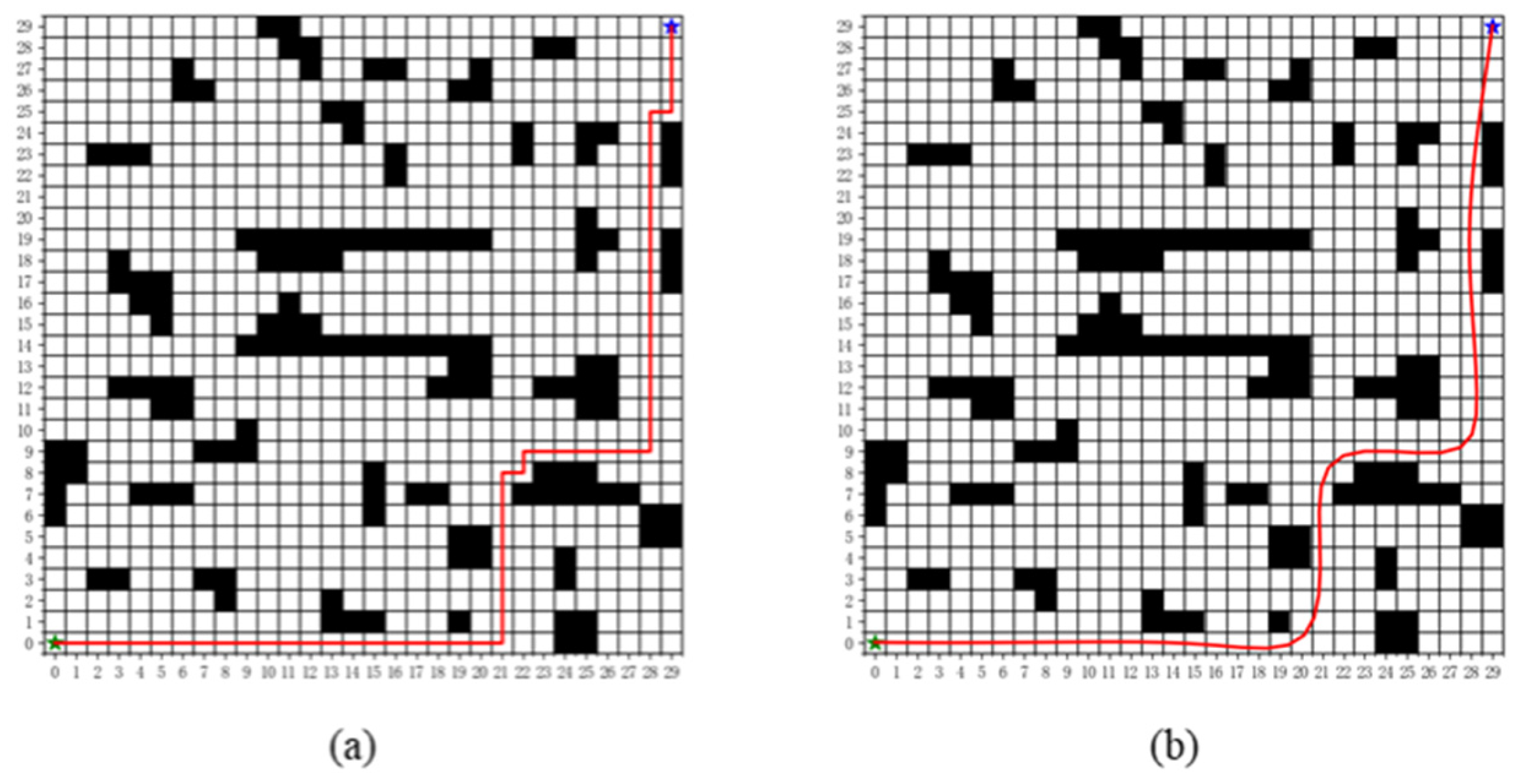
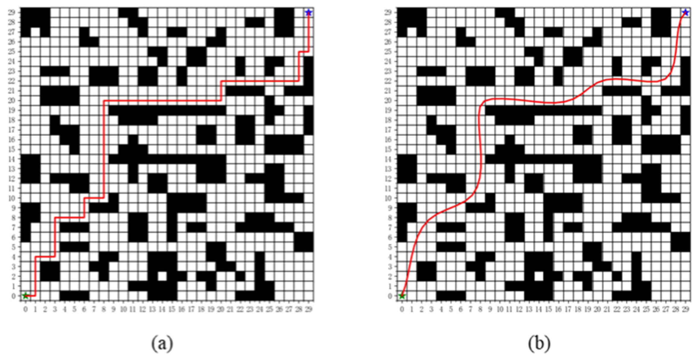
2.3.2. Path Smoothing

Although the pruning strategy eliminates redundant nodes in the path, the straight-line connections between nodes create abrupt directional changes that fail to satisfy the kinematic constraints of the robot. Therefore, further path optimisation is required. This paper employs the quasi-uniform cubic B-spline curve (with curve order k = 4, degree k − 1 = 3) to optimise the path, ensuring a high degree of consistency between the optimised path and the original trajectory.
The expression for the quasi-uniform B-spline curve is:
p ( u ) = i = 0 n p i · B i , k ( u ) , u [ u k , u k + 1 ]
where p ( u ) is the smoothed path point, u is the curve parameter; p i is the initial path point set, n is the number of path points; B i , k ( u ) is the k th-order ( k 1 ) B-spline basis function, k is the curve order, and i is the basis function index. The B-spline basis functions are defined via the Cox–deBoor recurrence formula:
B i , 0 ( u ) = 1 ,           u i u u i + 1 0 ,           e l s e
B i , k ( u ) = u u i u i + k u i · B i , k 1 ( u ) + u i + k + 1 u u i + k + 1 u i + 1 · B i + 1 , k 1 ( u )
The knot vector U = { u 0 , u 1 , u 2 , . . . . . , u n + k } is constructed as a quasi-uniform clamped vector, in which the start and end knots are repeated k times to ensure that the spline curve interpolates the first and last control points. Specifically, the knot vector is defined as:
U = 0,0 , 0,0 , 1,2 . . . . , n k + 1 , n k + 2 , n k + 2 , n k + 2 , n k + 2
To generate the final smoothed trajectory, the curve is sampled over the domain u [ u i , u i + 1 ) with a fixed parameter interval: Δ u = 0.01 , u j = u k + j · Δ u , j = 0,1 , . . . . . , N , where:
N = u n + 1 u k Δ u
Through the analysis of the above formula, it can be concluded that the characteristics of quasi uniform B-spline curves can be summarised as follows. On any node interval, there are at most k + 1 non-zero k-order basis functions. In the interval [ u i , u i + 1 ) , only the (ik) th path point to the i Path points are used for computation to give B-spline curves local variability. Based on these characteristics, this paper uses quasi uniform cubic B-spline curves for path smoothing, effectively eliminating abrupt points in the path and ensuring the continuity and smoothness of the trajectory.

2.4. Comparative Analysis of Improved A* Algorithms

To further verify the path planning performance of the improved A* algorithm in different environments, and at the same time to enhance the statistical validity of the experimental results, this paper conducts additional simulation experiments under random obstacle scenarios in addition to the original specific simple and complex environments. Specifically, two types of environments, simple (approximately 20% obstacle coverage) and complex (approximately 25% obstacle coverage), are constructed in a 30 × 30 grid map, with 30 randomly generated obstacle layouts for each type. In each group of scenarios, the starting point is set at (0, 0) and the end point at (29, 29). Both the traditional A* algorithm and the improved A* algorithm are employed for path planning, with the key metrics including the number of path points, turns, non-smooth turns, and the path lengths being recorded. The mean and standard deviation are then calculated. Figure 3 and Figure 4 present comparisons between the traditional A* algorithm and the improved A* algorithm* in randomly generated simple and complex environments, respectively, while the quantitative results are shown in Table 1.
The experimental results are shown in Table 1, demonstrating that the improved A* algorithm exhibits significant advantages in both types of environments. Compared with the traditional A*, in the simple environment, the number of path points is reduced by approximately 86.2% on average, the number of turn points is reduced by approximately 43%, the non-smooth turn points are all eliminated, and the path length is reduced by approximately 2.1% on average. In the complex environment, the number of path points is reduced by approximately 88% on average, the number of turn points is reduced by approximately 61.4%, the number of non-smooth turn points is 0, and the path length is reduced by approximately 15.6% on average. Furthermore, the reduction in standard deviation indicates that the improved algorithm has enhanced stability and generalisation ability across diverse map structures. It can be seen that the improved A* algorithm not only effectively simplifies the path structure but also maintains high robustness and smoothness in a variety of environments.

3. Smoothing Optimisation A*-Guided DWA

3.1. DWA Algorithm

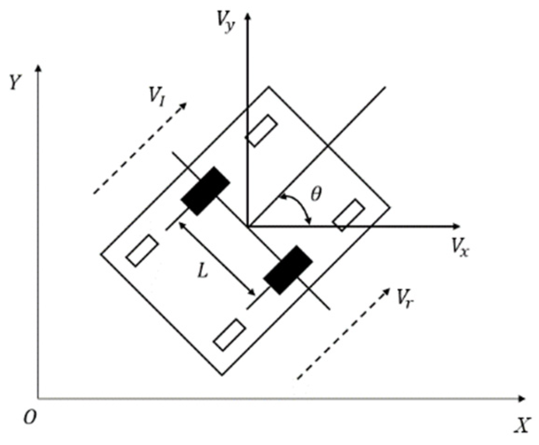
3.1.1. Vehicle Kinematics Modelling

The mobile robot investigated in this paper features a front-wheel differential drive with rear-wheel omnidirectional support, which belongs to the typical two-wheel differential motion model. The simplified model is shown in Figure 5.
Assuming that the current momentary position of the robot is [ x ( t ) , y ( t ) , θ ( t ) ] , where ( x ( t ) , y ( t ) ) is the position and θ ( t ) is the heading angle, the robot’s motion is described under constant linear velocity v ( t ) and angular velocity ω ( t ) during the sampling time interval Δ t (in seconds). The displacement increment of the robot during the sampling time interval Δ t can be expressed as:
Δ x = v ( t ) · Δ t · c o s ( θ ( t ) ) Δ y = v ( t ) · Δ t · s i n ( θ ( t ) ) Δ θ = ω ( t ) · Δ t
The position of the mobile robot at the next sampling interval can be represented as:
x ( t + Δ t ) = x ( t ) + Δ x y ( t + Δ t ) = y ( t ) + Δ y θ ( t + Δ t ) = θ ( t ) + Δ θ

3.1.2. Speed Sampling

In practice, the speed of a mobile robot is affected by the following three factors:
(1)
Maximum speed and minimum speed
The speed limit of the mobile robot originates from its power system, where the maximum speed represents the fastest speed at which the vehicle can operate stably, and the minimum speed denotes the slowest speed at which the vehicle can still maintain control at low speeds. The set of the vehicle velocity and the angular velocity of the pendulum v s is:
v s = ( v , ω ) | v [ v m i n , v m a x ] , ω [ ω m i n , ω m a x ]
(2)
Motor performance
The motor of the mobile robot directly determines the power output and motion capability of the vehicle, and its speed constraint formula is shown in Equation (11):
v d = ( v , ω ) | v [ v 0 v ˙ n Δ t , v 0 + v ˙ m Δ t ] , ω [ ω 0 ω ˙ n Δ t , ω 0 + ω ˙ m Δ t ]
(3)
Obstacles
The mobile robot needs to stop before hitting an obstacle with a maximum deceleration that satisfies the following constraints:
v a = ( v , ω ) | v 2 d i s t ( v , ω ) v ˙ n , ω 2 d i s t ( v , ω ) ω ˙ n
The final velocity is taken as the intersection of v s , v d and v a , and the space of desirable velocities for the mobile robot is denoted by v f , which takes the value:
v f = v s v d v a
The parameters in Equations (10)–(13) are shown in Table 2:

3.1.3. Evaluation Function for DWA

The evaluation function of the DWA algorithm is used to assess the quality of the trajectory generated at a given moment in time for a given pair of velocities, both linear and angular. The metrics of the evaluation function include azimuth, gap and velocity, and the evaluation function is:
G v , ω = σ · ( α · h e a d i n g ( v , ω ) + β · v e l ( v , ω ) + γ · d i s t ( v , ω ) )
In Equation (14), h e a d i n g ( v , ω ) is the direction angle evaluation index for assessing the consistency of the current direction with the target direction; d i s t ( v , ω ) is the distance between the current trajectory and the nearest obstacle; and v e l ( v , ω ) is the current velocity evaluation function for evaluating the smoothing and feasibility of the current velocity pair. α , β and γ are the weighting coefficients of the three evaluation metrics. In order to avoid one of the values being too large and too dominant, the evaluation function is obtained by smoothing, multiplying by the corresponding coefficients and summing up, and finally, the objective function is normalised using the smoothing factor σ .

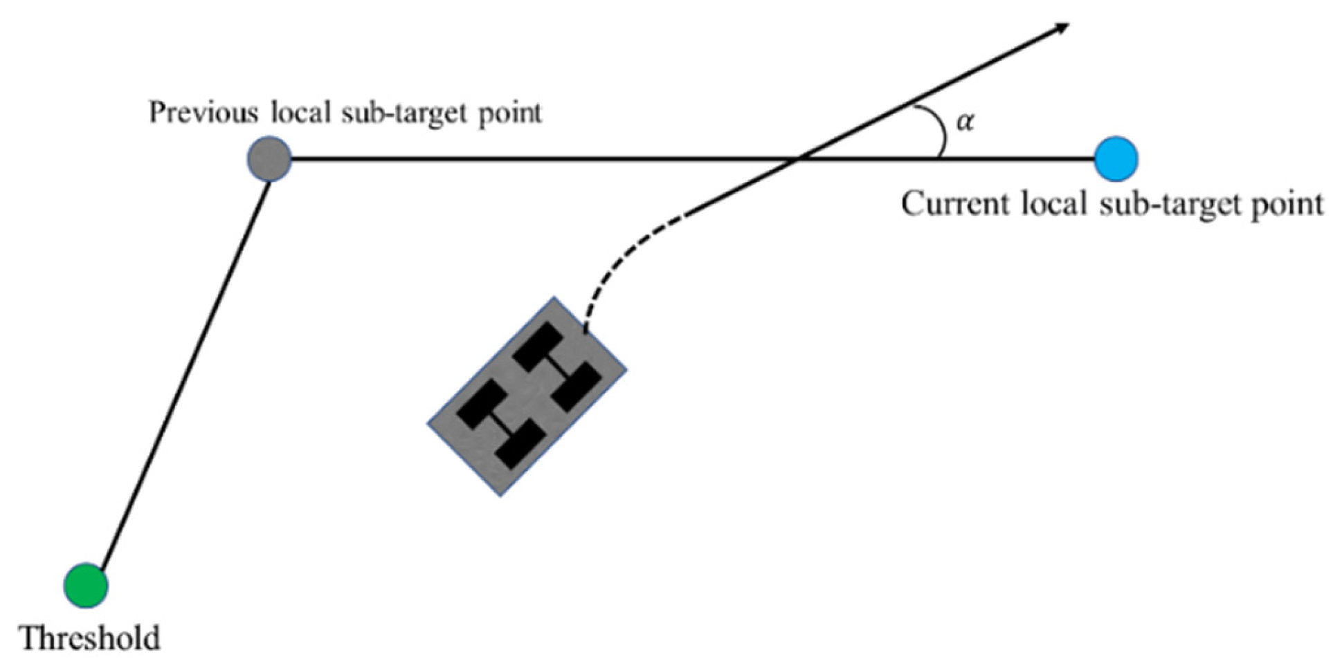
3.2. Enhanced Global Path Constraints

In order to solve the problem that the local path planned by DWA will deviate from the global path during obstacle avoidance, the evaluation function of the DWA algorithm is improved. The improved algorithm adds two evaluation subfunctions: the distance evaluation subfunction p a t h d i s t ( v , ω ) between the reference trajectory and the global path, and the path direction evaluation subfunction p a t h h e a d i n g ( v , ω ) . The corresponding coefficients are μ and φ , the trajectory with the lowest cost of the evaluation function is the optimal trajectory, and the evaluation function can be rewritten as:
G v , ω = σ · ( α · h e a d i n g ( v , ω ) + β · v e l ( v , ω ) + γ · d i s t ( v , ω ) + μ · p a t h d i s t ( v , ω ) + φ · p a t h h e a d i n g ( v , ω ) )
(1)
Evaluation subfunction of the distance between the reference trajectory and the global path
The smaller the deviation distance between the end point of the trajectory to be evaluated and the global path, the lower the deviation of the trajectory from the global path. This evaluation term uses the point-to-straight-line distance formula to calculate the deviation distance between the end point and the global path. As shown in Figure 6, a schematic diagram of the distance evaluation subfunction of the reference trajectory from the global path is shown. The calculation process of the distance evaluation subfunction between the reference trajectory and the global path is shown in Equations (16) and (17), where ( x 0 , y 0 ) denotes the coordinates of the end point of the trajectory to be evaluated calculated based on the robot kinematics model, and A, B, and C are the coefficients in the equation y = A · x + B · y + C that connects the robot’s current local target point to the previous local target point.
d i s t a n c e = A · x 0 + B · y 0 + C A 2 + B 2
p a t h d i s t ( v , ω ) = c o s | d i s t a n c e | ,     d i s t a n c e π 2 0 ,     d i s t a n c e > π 2
(2)
Path direction evaluation
The main function of the path direction evaluation subfunction is to ensure that the motion direction of the mobile robot is always consistent with the global path, so as to improve the directional stability during the motion process. The subfunction determines whether the end of the trajectory is aligned with the direction of the global path by calculating the current direction of the global path and evaluating the size of the angle between the end of the trajectory to be evaluated and the direction. A schematic diagram of the path direction evaluation subfunction is shown in Figure 7.
The specific calculation formula of the path direction evaluation subfunction is shown in Equation (18). α is the angle between the end of the trajectory to be evaluated and the global path direction, and the smaller the α , the smaller the deviation of the robot’s motion direction from the global path direction, and the higher the score of this evaluation item.
p a t h h e a d i n g ( v , ω ) = π α

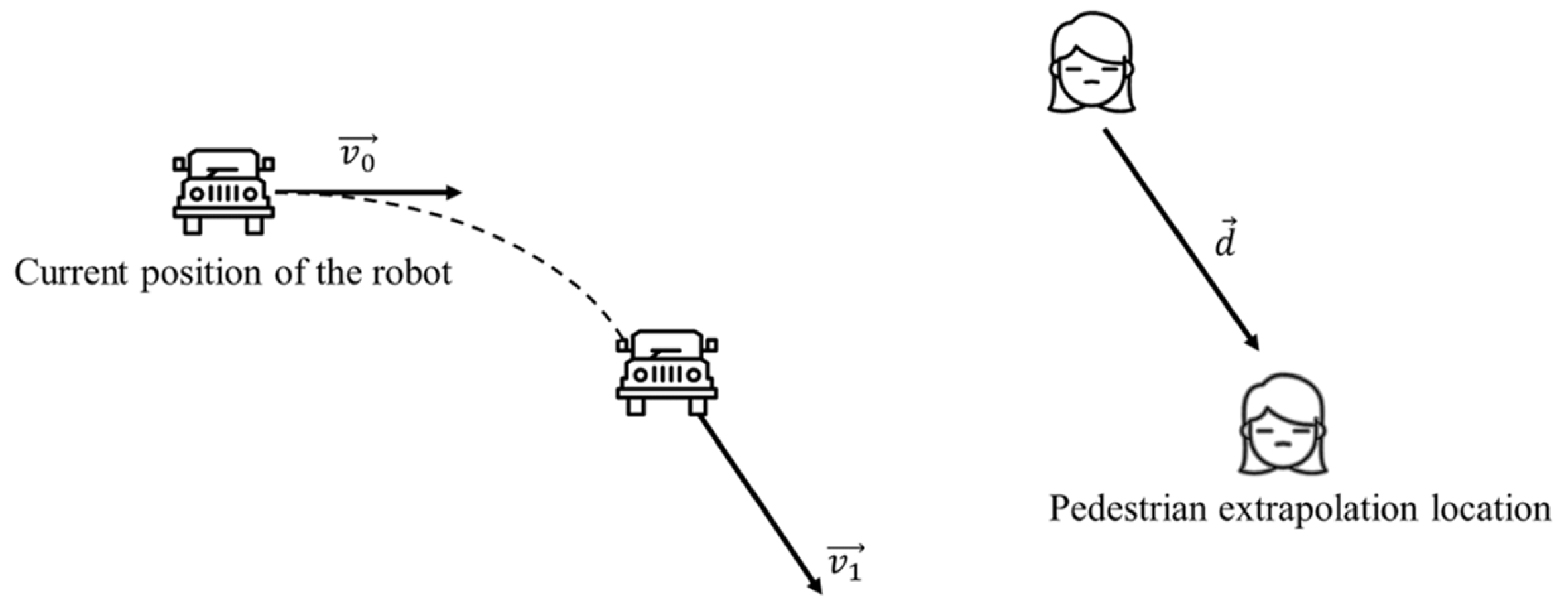
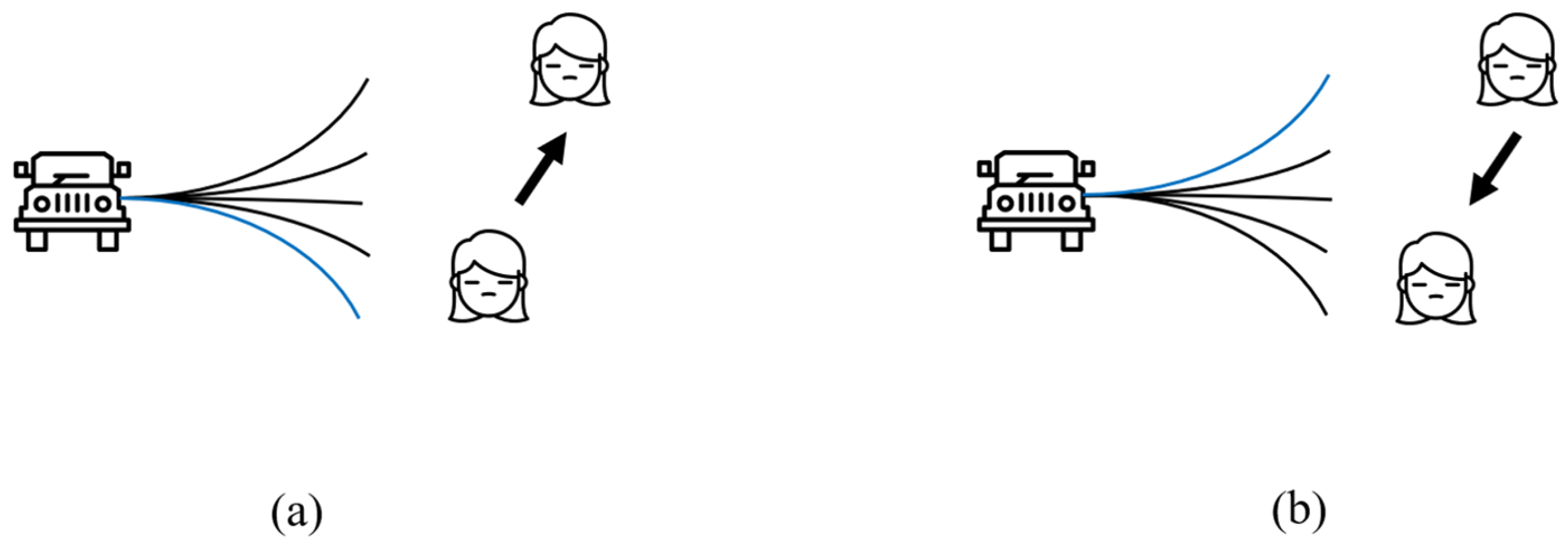
3.3. Optimisation of Obstacle Avoidance Efficiency

In order to solve the problem of low efficiency of the DWA algorithm in avoiding dynamic obstacles, the evaluation function is further improved by adding a new dynamic obstacle avoidance evaluation subfunction d y n a m i c ( v , ω ) , with corresponding coefficients of τ . This subfunction takes into account the relative relationship between the end of the mobile robot’s aerial plane and the direction of pedestrians walking, so as to optimise the obstacle avoidance strategy. A schematic diagram of this subfunction is shown in Figure 8.
Based on the relative relationship between the pedestrian walking direction deduced from the end of the trajectory corresponding to the speed in the DWA window, the d y n a m i c ( v , ω ) function term is designed as Equation (19), where v 0 is the vector of velocities corresponding to the current direction of motion, v 1 is the vector of velocities corresponding to the direction of the end of the predicted trajectory, d is the pedestrian walking direction vector.
d y n a m i c ( v , ω ) = θ ( v 1 , d ) ,     θ ( v 0 , d ) < π 2 π θ ( v 1 , d ) ,     θ ( v 0 , d ) π 2
When ( v 0 , d ) < π 2 holds, it means that the mobile robot has a tendency to move in the same direction as the pedestrians, and at this time, the trajectory with a larger value of ( v 1 , d ) should be chosen so that the robot will move in the direction away from the pedestrian’s movement, as shown in Figure 9a. When ( v 0 , d ) π 2 holds, it indicates that the robot has a tendency to move in the opposite direction to the pedestrians, and then the trajectory with a smaller value of ( v 1 , d ) should be selected so that the robot moves in the direction away from the pedestrian motion, as shown in Figure 9b.

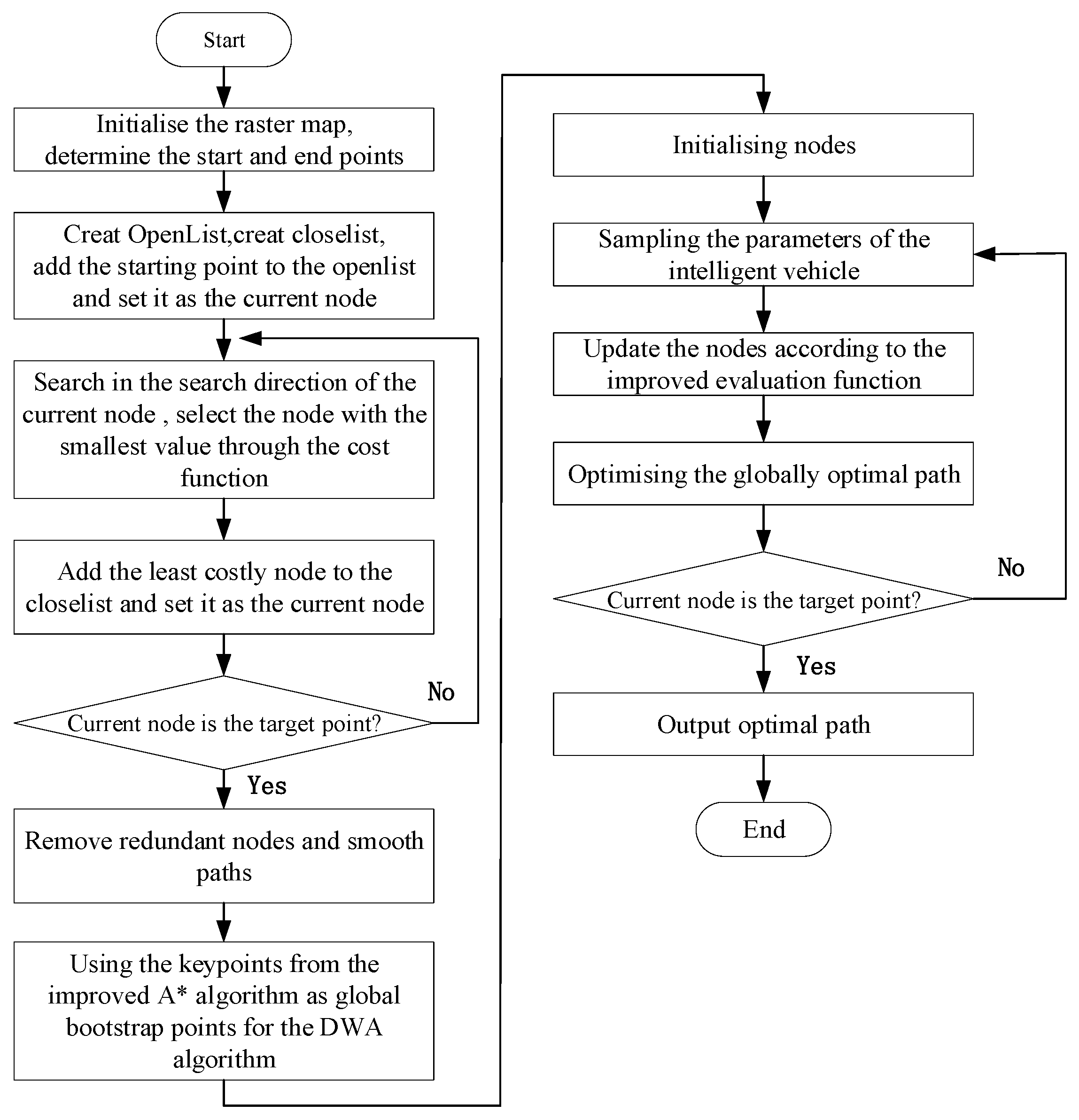
4. Steps and Processes of SOA-DWA Algorithm

The SOA-DWA algorithm flow is as follows:
Step1: Initialise the raster map and determine the start and end points of the mobile robot.
Step2: Adopt the improved A* algorithm for global path planning, establish the CLOSE table and OPEN table, and select the node with the smallest cost near the current node to join the CLOSE table through the cost function, and set it as the current node.
Step3: Judge whether the vehicle has travelled to the target point. If it has arrived at the target point, the execution of A* algorithm ends and continues to execute Step4; if it has not arrived at the target point, it returns to continue to execute Step2.
Step4: Remove redundant nodes, smooth the path, and take the key point after improving A* algorithm as the global guidance point of DWA algorithm.
Step5: Local path planning by the improved DWA algorithm to avoid obstacles and return to the global path after obstacle avoidance is completed.
The flowchart of SOA-DWA algorithm is shown in Figure 10.

5. Simulation Experiments and Analyses

The experimental environment used: Windows 10 system, 2.6 GHz i5-13500H CPU, 16 G RAM, with Python (version 3.11.4) as the programming language and Visual Studio Code(version 1.101) as the development environment. Additionally, the mobile robot is equipped with an Intel Core i7 processor running Ubuntu 20.04 and Ros1.

5.1. Ablation Study

To evaluate the contribution of each improvement in the proposed SOA-DWA algorithm, we conducted an ablation study in a consistent experimental setting. This study aims to isolate and quantify the impact of key modules including path pruning, path smoothing, and additional cost terms introduced in the DWA evaluation function. All experiments were conducted on the same static and dynamic map scenarios to ensure effective comparison.
The baseline model includes the traditional A* and DWA algorithms without any modification. Subsequently, pruning is implemented to eliminate redundant nodes and reduce unnecessary turns. Following this, B-spline smoothing is applied to the pruned path to enhance curvature continuity and ensure the trajectory better aligns with the robot’s kinematic constraints. For the DWA evaluation function, the impact of each additional cost term is evaluated separately.
To ensure the statistical reliability of the experimental results, each algorithm combination is run 30 times independently in each scenario, with each key performance indicator recorded, including path length, number of turning points, total turning angles, and running time. The results are summarised as “mean ± standard deviation” and presented in Table 3 and Table 4. The results show that pruning alone can significantly reduce both the path length and turning points. Following B-spline smoothing, the total turning angle is further reduced, indicating that the trajectory smoothness is significantly improved. On the other hand, adding the global path constraint to the original DWA significantly improves the consistency of the trajectory with the global path. And adding the obstacle avoidance strategy significantly reduces the search time.
These results clearly demonstrate the effectiveness of each proposed module and validate the necessity of their integration. The ablation study provides compelling evidence that each design decision contributes meaningfully to the overall performance gains achieved by the SOA-DWA algorithm.

5.2. Validation of Algorithm Effectiveness

In order to comprehensively evaluate the effectiveness of the proposed SOA-DWA algorithm, this paper further employs Monte Carlo simulation based on the original example scenarios, conducts 30 independent experiments under each type of scenario, and statistically analyses the key performance indicators of each type of algorithm to enhance the statistical significance of the experimental results.
The experiments are conducted in three typical scenarios: static known scenario, static unknown scenario, and dynamic unknown scenario. The traditional A*, traditional DWA and SOA-DWA algorithms were run in each scenario, and the obstacle layout and starting and stopping points were kept the same in each experiment, with only a small perturbation in the dynamic obstacle trajectory or initial conditions to simulate a more realistic random environment. For each experiment, we counted the key metrics such as path length, number of turning points, number of non-smooth turning points, and total turning angle, and calculated their mean and standard deviation.
Figure 11, Figure 12 and Figure 13 show some representative trajectory maps generated by the experiments in the three scenarios, and Table 5 further gives the comprehensive performance comparison of different algorithms under multiple simulations.
The statistical results demonstrate that the proposed SOA-DWA algorithm consistently outperforms the traditional DWA and A* algorithms across all test scenarios. In the static known scenarios, SOA-DWA achieves significant reductions in both the number of turning points and the total turning angle compared to A* and DWA, especially in Scenario 2, where it reduces the total turning angle by approximately 10.6% compared to DWA and 32.7% compared to A*. Moreover, all non-smooth turning points are eliminated in the SOA-DWA results, indicating an effective smoothing capability that contributes to more feasible and comfortable trajectories for real-world navigation.
Since the A* algorithm cannot achieve obstacle avoidance when dealing with unknown obstacles, the simulation results of the A* algorithm in an unknown scenario cannot be given. In the static unknown scenarios, although the obstacle layout is not fully known in advance, SOA-DWA still maintains stable performance. For example, in Scenario 2, it shortens the average path length by approximately 3.7% compared to DWA, while also reducing the total turning angle and number of turns, which suggests that SOA-DWA is capable of real-time adaptive optimisation even under partial information conditions.
In the dynamic unknown scenarios, where obstacle movement is unpredictable, SOA-DWA further demonstrates its robustness and adaptability. In Scenario 2, SOA-DWA reduces the total turning angle by 18.8% and the path length by 3.9% compared to DWA. Notably, the number of turning points is significantly reduced, which implies that the planned path is not only shorter but also smoother and more stable when responding to dynamic changes in the environment.
Based on the above data, one-way analysis of variance (ANOVA) and paired independent samples t-tests were performed on the four metrics, namely, path length, number of turning points, number of non-smoothed turning points, and total turning angle. The analyses show that the SOA-DWA algorithm exhibits significantly better performance differences than the traditional A* and DWA algorithms in all metrics (p-values are all much less than 0.05). In particular, in dynamic unknown environments, its path length and corner differences are significant compared to the traditional DWA algorithm, indicating that the proposed fusion algorithm has better obstacle avoidance capability and path stability in dynamic environments.

5.3. Comparative Analysis of Algorithm Performance

In order to verify the performance of the SOA-DWA algorithm, in the simulation comparison experiments shown in Figure 14, this paper introduces a unified evaluation index system, including path length, search time, path smoothness, and obstacle avoidance efficiency, to comprehensively evaluate the algorithm’s path optimisation capability, real-time performance and obstacle avoidance stability. Under the same experimental conditions, the SOA-DWA algorithm is quantitatively compared and analysed with the fusion algorithms in [24,25], and the experimental results are shown in Figure 15.
From Figure 14 and Figure 15, it can be seen that in dynamic and static scenario 1, the SOA-DWA algorithm reduces the path length by 13.8% and 7.5%, reduces the search time by 38% and 47%, and improves the smoothing degree by 26% and 16.7%, respectively, compared with the algorithms in [24,25], which effectively improves the distances to the added obstacles; in dynamic and static scenario 2, the path length reduces the path length by 12.1% and 7%, and the search time by 37.8% and 46%, respectively, and the search time is reduced by 37.8% and 46%, and the smoothness is improved by 31.4% and 19.3%, respectively. Specifically, the lack of constraints on the locally planned paths in the algorithms of [24,25] leads to their deviation from the globally optimal paths and the lack of fine-grained optimisation of the local paths during the dynamic obstacle avoidance process, which affects the efficiency of the planned obstacle avoidance. In contrast, by combining the global path planning algorithm and the local path planning algorithm, the SOA-DWA algorithm dynamically corrects the local paths on the basis of the globally optimal paths, which not only significantly shortens the path length and search time, but also effectively improves the obstacle avoidance efficiency by adjusting the robot’s trajectory in real time. The experimental results show that the SOA-DWA algorithm is able to respond quickly to environmental changes and maintain a safe distance from obstacles during the dynamic obstacle avoidance process, and at the same time reduces the number of path turns, which further improves the smoothness and safety of the path planning, and fully reflects its superiority in complex environments.

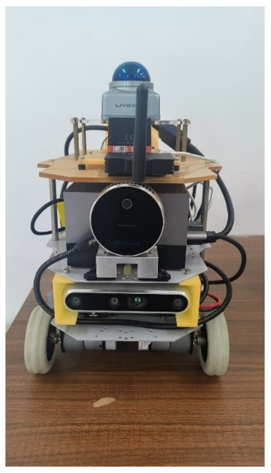
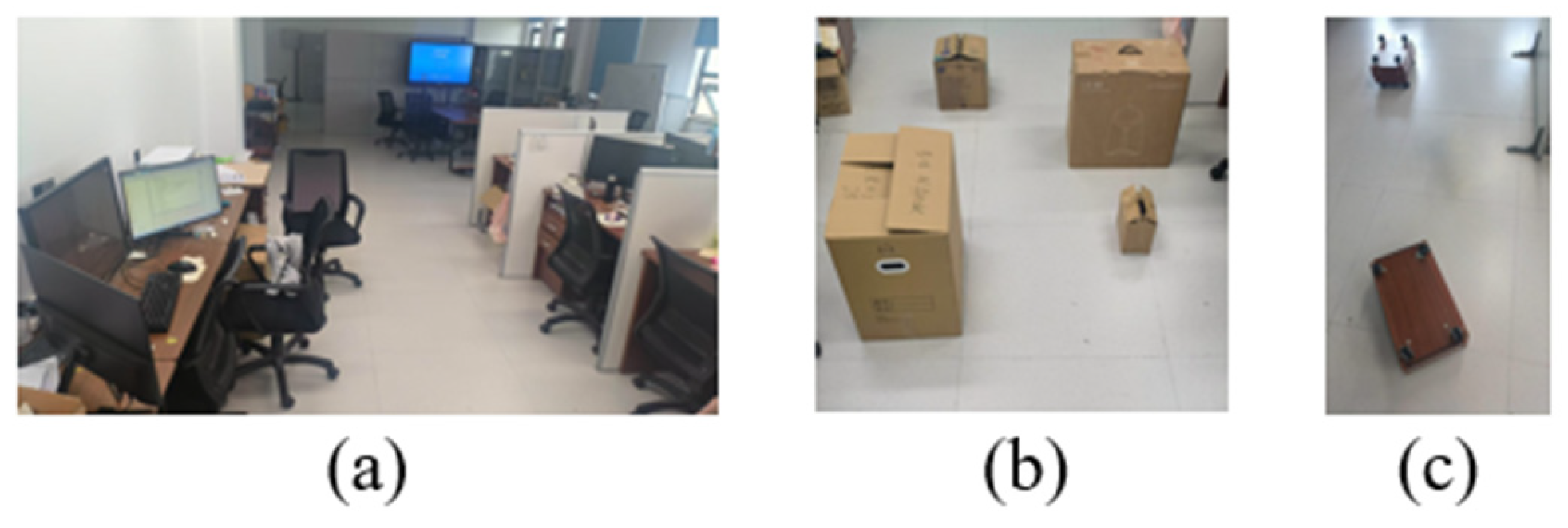
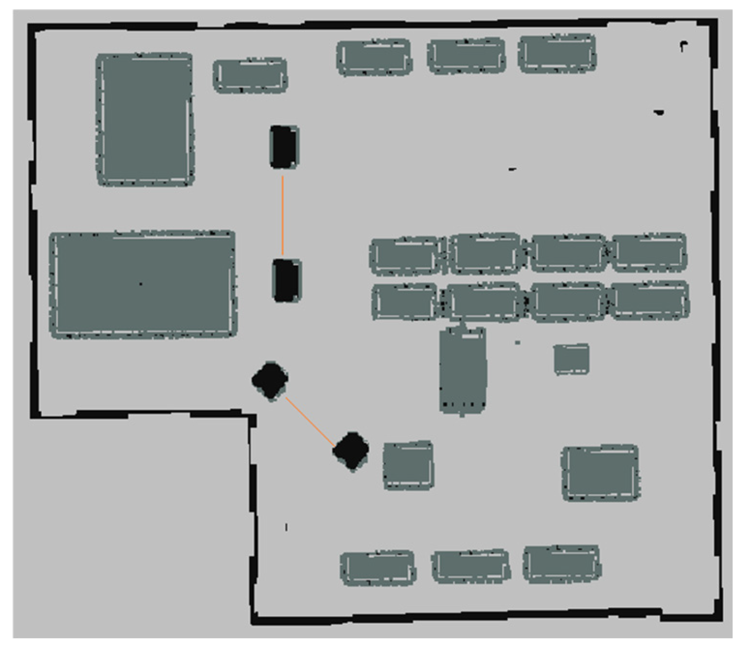
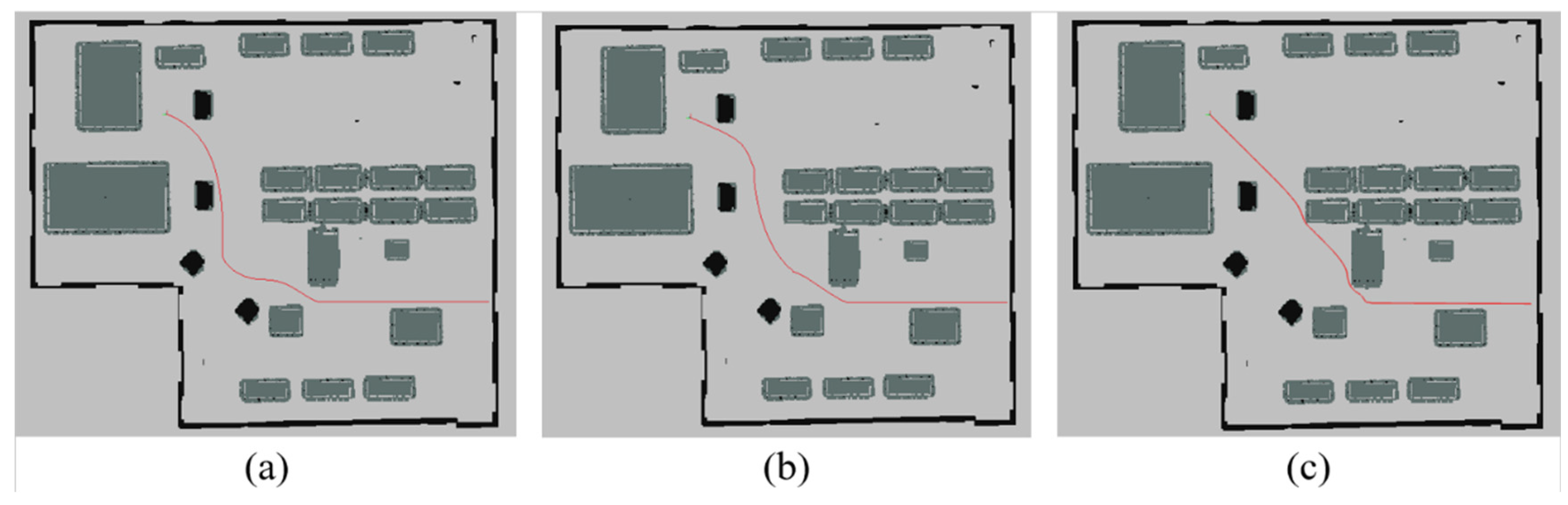
5.4. Mobile Robot Experiment

In order to verify the performance of the SOA-DWA algorithm in real-world scenarios, this paper conducts a real-world experiment using the mobile robot platform shown in Figure 16. The robot senses its surroundings through laser radar and camera sensor, the power system consists of high-performance servo motors and gearboxes, and the power management system consists of an on-board control board that manages the power supply to the vehicle.
To ensure rigorous consistency between experimental and simulation results, we implement a systematic verification protocol comprising four key phases: first, based on the simulation model, we build a physical test site in a 1:1 ratio in the physical environment, including wall structure and obstacle layout; then we strictly unify the starting and ending coordinate systems of the test tasks to ensure consistency in the spatial reference; then, we synchronize the dynamic characteristics of the simulation environment with the actual navigation algorithm configuration in real time through the parameter calibration platform; finally, we use dynamic environment modeling technology to dynamically match the obstacle distribution, terrain features and scenario complexity of the test site with the digital simulation, thereby building a full-link verification system from virtual to physical, providing systematic guarantees for the credibility of the experimental results. The actual scenario is shown in Figure 17, and the simulation scenario built by Gazebo and visualised by Rviz is shown in Figure 18.
As shown in Figure 19, the algorithm of [24], the algorithm of [25] and the algorithm of this paper were tested to generate the length of the trajectory, the angle of the turn and the time of the planning, respectively. In order to ensure the accuracy of the experiment, the three algorithms were run 10 times, and the relevant data were statistically analysed, and the final experimental results are shown in Table 6, which can effectively avoid the bias and error in the experiment, and ensure the reliability and validity of the experimental results.
Experiments on the mobile robot show that the SOA-DWA algorithm proposed in this paper exhibits significant advantages in terms of path length, turning angle and path planning time, which further validates the effectiveness of the improved algorithm proposed in this paper.

6. Conclusions

In this study, we propose a fusion algorithm, SOA-DWA, which introduces path pruning and path smoothing strategies into the traditional A* algorithm, significantly solving the problems of high path redundancy and poor smoothness in the A* algorithm. Global path constraint and optimisation strategies are introduced into the DWA algorithm. This aims to address two issues: the deviation from the global optimal path when integrating global planning, and the low efficiency of dynamic obstacle avoidance in mobile robots.
Simulation and real vehicle experimental results show that the SOA-DWA algorithm can effectively avoid both static and dynamic obstacles. At the same time, it remains aligned with the global optimal path in scenarios with different levels of complexity.

Author Contributions

Conceptualization, L.T. and L.C.; methodology, L.T.; software, L.T.; validation, G.Z., Q.S. and S.C.; formal analysis, S.C.; investigation, Q.S.; resources, G.Z.; data curation, L.C.; writing—original draft preparation, L.T.; writing—review and editing, L.T.; visualization, L.T.; supervision, S.C.; project administration, L.C.; funding acquisition, S.C. All authors have read and agreed to the published version of the manuscript.

Funding

This work was supported in part by the National Key Research and Development Program of China under Grant 2023YFD2401302; in part by Shanghai Chongming District Agricultural Science and Innovation Project under Grant 2021CNKC-05-06; and in part by Shanghai Agricultural Science and Technology Innovation Project (Shanghai Agricultural Science and Technology) under Grant I2023006.

Institutional Review Board Statement

Not applicable.

Informed Consent Statement

Not applicable.

Data Availability Statement

Data are contained within the article. The data presented in this study can be requested from the authors.

Acknowledgments

Thanks to the School of Engineering of Shanghai Ocean University for providing the mobile robot hardware and experimental facilities for this study.

Conflicts of Interest

The authors declare no conflicts of interest.

References

  1. Zhou, T.; Wei, W. Mobile robot path planning based on an improved ACO algorithm and path optimization. Multimed. Tools Appl. 2024, 84, 10899–10922. [Google Scholar] [CrossRef]
  2. Dang, T.-V.; Tan, P.X. Hybrid Mobile Robot Path Planning Using Safe JBS-A*B Algorithm and Improved DWA Based on Monocular Camera. J. Intell. Robot. Syst. 2024, 110, 151. [Google Scholar] [CrossRef]
  3. Cao, S.; Sui, G.; Zhou, G. Path tracking control with delay characteristics for unmanned vehicles in aquaculture workshops. J. Fish. China 2024, 48, 133–144. [Google Scholar]
  4. Katona, K.; Neamah, H.A.; Korondi, P. Obstacle Avoidance and Path Planning Methods for Autonomous Navigation of Mobile Robot. Sensors 2024, 24, 3573. [Google Scholar] [CrossRef] [PubMed]
  5. Galarza-Falfan, J.; García-Guerrero, E.; Aguirre-Castro, O.; Lopez-Bonilla, O.; Tamayo Pérez, U.; Cárdenas-Valdez, J.; Hernández-Mejía, C.; Borrego-Dominguez, S.; Inzunza Gonzalez, E. Path Planning for Autonomous Mobile Robot Using Intelligent Algorithms. Technologies 2024, 12, 82. [Google Scholar] [CrossRef]
  6. Paden, B.; Čáp, M.; Yong, S.Z.; Yershov, D.; Frazzoli, E. A Survey of Motion Planning and Control Techniques for Self-Driving Urban Vehicles. IEEE Trans. Intell. Veh. 2016, 1, 33–55. [Google Scholar] [CrossRef]
  7. Lun, Q.; Luxin, H.; Boyu, Z.; Shaojie, S.; Fei, G. Survey of UAV motion planning. IET Cyber-Syst. Robot. 2020, 2, 14–21. [Google Scholar]
  8. Xu, X.; Zeng, J.; Zhao, Y.; Lü, X. Research on global path planning algorithm for mobile robots based on improved A*. Expert Syst. Appl. 2024, 243, 122922. [Google Scholar] [CrossRef]
  9. Xing, S.; Fan, P.; Ma, X.; Wang, Y. Research on robot path planning by integrating state-based decision-making A* algorithm and inertial dynamic window approach. Intell. Serv. Robot. 2024, 17, 901–914. [Google Scholar] [CrossRef]
  10. Zhu, D.D.; Sun, J.Q. A New Algorithm Based on Dijkstra for Vehicle Path Planning Considering Intersection Attribute. IEEE Access 2021, 9, 19761–19775. [Google Scholar] [CrossRef]
  11. Ma, G.; Duan, Y.; Li, M.; Xie, Z.; Zhu, J. A probability smoothing Bi-RRT path planning algorithm for indoor robot. Future Gener. Comput. Syst. 2023, 143, 349–360. [Google Scholar] [CrossRef]
  12. Ganesan, S.; Ramalingam, B.; Mohan, R.E. A hybrid sampling-based RRT* path planning algorithm for autonomous mobile robot navigation. Expert Syst. Appl. 2024, 258, 125206. [Google Scholar] [CrossRef]
  13. Orozco-Rosas, U.; Picos, K.; Pantrigo, J.J.; Montemayor, A.S.; Cuesta-Infante, A. Mobile Robot Path Planning Using a QAPF Learning Algorithm for Known and Unknown Environments. IEEE Access 2022, 10, 84648–84663. [Google Scholar] [CrossRef]
  14. Bonny, T.; Kashkash, M. Highly optimised Q-learning-based bees approach for mobile robot path planning in static and dynamic environments. J. Field Robot. 2021, 39, 317–334. [Google Scholar] [CrossRef]
  15. Gong, X.; Gao, Y.; Wang, F.; Zhu, D.; Zhao, W.; Wang, F.; Liu, Y. A Local Path Planning Algorithm for Robots Based on Improved DWA. Electronics 2024, 13, 2965. [Google Scholar] [CrossRef]
  16. Wu, L.; Huang, X.; Cui, J.; Liu, C.; Xiao, W. Modified adaptive ant colony optimisation algorithm and its application for solving path planning of mobile robot. Expert Syst. Appl. 2023, 215, 119410. [Google Scholar] [CrossRef]
  17. Xiong, N.; Zhou, X.; Yang, X.; Xiang, Y.; Ma, J. Mobile Robot Path Planning Based on Time Taboo Ant Colony Optimisation in Dynamic Environment. Front. Neurorobot. 2021, 15, 642733. [Google Scholar] [CrossRef]
  18. Hu, M.; Li, X.; Ren, Z.; Zeng, S. Three-dimensional path planning for UAVs based on A* algorithm with improved heuristic function. Acta Armamentarii 2024, 45, 302–307. [Google Scholar]
  19. Yan, J.; Liu, C.; Sun, H.; Chen, X. Research on path planning algorithm for mobile robots based on improved A* fused with DWA. J. Yuncheng Univ. 2024, 42, 45–51. [Google Scholar]
  20. Sun, Y.; Wang, R.; Jiang, D. Dynamic path planning for surface vessels based on fusion of A* and DWA algorithms. Chin. J. Sci. Instrum. 2024, 45, 301–310. [Google Scholar]
  21. Liu, L.; Wang, X.; Wang, X.; Xie, J.; Liu, H.; Li, J.; Wang, P.; Yang, X. Path Planning and Tracking Control of Tracked Agricultural Machinery Based on Improved A* and Fuzzy Control. Electronics 2024, 13, 188. [Google Scholar] [CrossRef]
  22. Lai, R.; Wu, Z.; Liu, X.; Zeng, N. Fusion Algorithm of the Improved A* Algorithm and Segmented Bézier Curves for the Path Planning of Mobile Robots. Sustainability 2023, 15, 2483. [Google Scholar] [CrossRef]
  23. He, L.; Ning, Z.; Yuan, L.; Liu, Z. Path planning for service robots using socially constrained adaptive dynamic window approach. J. Xi’an Jiaotong Univ. 2024, 58, 42–51. [Google Scholar]
  24. Huang, J.; Chen, X. Research on robot fusion algorithm based on improved A* and DWA. Chin. J. Sens. Actuators 2024, 37, 2043–2049. [Google Scholar]
  25. Zhang, Y.; Li, B.; Huo, T.; Liu, T. Research on robot dynamic obstacle avoidance method combining improved A* algorithm with DWA algorithm. J. Syst. Simul. 2025, 1, 1–10. [Google Scholar]
Figure 1. Raster environment: (a) 30 × 30 simple environment; (b) 30 × 30 complex environments.
Applsci 15 06956 g001
Figure 2. A* algorithmic planning path.
Applsci 15 06956 g002
Figure 3. Comparison of algorithm improvement in simple scenarios. (a) Traditional A* algorithm for path planning in simple scenario; (b) improved A* algorithm for path planning in simple scenario.
Applsci 15 06956 g003
Figure 4. Comparison of algorithm improvement in complex scenarios. (a) Traditional A* algorithm for path planning in complex scenario; (b) improved A* algorithm for path planning in complex scenario.
Applsci 15 06956 g004
Figure 5. Mobile robot motion modelling.
Applsci 15 06956 g005
Figure 6. Schematic of the distance between the reference trajectory and the global path.
Applsci 15 06956 g006
Figure 7. Schematic diagram of heading deviation.
Applsci 15 06956 g007
Figure 8. Schematic diagram of dynamic obstacle avoidance evaluation subfunction.
Applsci 15 06956 g008
Figure 9. Schematic of the DWA algorithm’s preferred trajectory. (a) Same trends between mobile robots and pedestrians; (b) different trends between mobile robots and pedestrians.
Applsci 15 06956 g009
Figure 10. Flowchart of SOA-DWA algorithm.
Applsci 15 06956 g010
Figure 11. Simulation results in static scenarios. (a) Traditional A* algorithm in scenario 1; (b) DWA algorithm in scenario 1; (c) SOA-DWA algorithm in scenario 1; (d) traditional A* algorithm in scenario 2; (e) DWA algorithm in scenario 2; (f) SOA-DWA algorithm in scenario 2.
Applsci 15 06956 g011
Figure 12. Simulation results in unknown static scenarios. (a) DWA algorithm in scenario 1; (b) SOA-DWA algorithm in scenario 1; (c) DWA algorithm in scenario 2; (d) SOA-DWA algorithm in scenario 2.
Applsci 15 06956 g012
Figure 13. Simulation results in unknown dynamic scenarios. (a) DWA algorithm in scenario 1; (b) SOA-DWA algorithm in scenario 1; (c) DWA algorithm in scenario 2; (d) SOA-DWA algorithm in scenario 2.
Applsci 15 06956 g013
Figure 14. Experimental comparison of different algorithms. (a) Algorithm from [24] in scenario 1; (b) algorithm from [25] in scenario 1; (c) SOA-DWA algorithm in scenario 1; (d) algorithm from [24] in scenario 2; (e) algorithm from [25] in scenario 2; (f) SOA-DWA algorithm in scenario 2.
Applsci 15 06956 g014
Figure 15. Comparative data of simulation experiments under dynamic and static scenarios. (a) Experimental comparison data in scenario 1; (b) experimental comparison data in scenario 2 [24,25].
Applsci 15 06956 g015
Figure 16. Mobile robot platform.
Applsci 15 06956 g016
Figure 17. Experimental environment. (a) Actual scenario; (b) static obstacles; (c) dynamic obstacles.
Applsci 15 06956 g017
Figure 18. Simulation environment.
Applsci 15 06956 g018
Figure 19. Paths generated by different algorithms. (a) Algorithm from [24]; (b) algorithm from [25]; (c) SOA-DWA algorithm.
Applsci 15 06956 g019
Table 1. Performance comparison of A* algorithm before and after improvement.
EnvironmentAlgorithmNumber of Path Points (Mean ± Standard Deviation)Number of Turning Points (Mean ± Standard Deviation)Number of Nonsmooth Turning Points (Mean ± Standard Deviation)Path Length (Mean ± Standard Deviation)/m
Simple EnvironmentTraditional A* algorithm60.1 ± 1.27.2 ± 0.47.0 ± 0.257.2 ± 0.9
Improved A* algorithm8.3 ± 0.34.1 ± 0.20 ± 055.98 ± 0.7
Complex EnvironmentTraditional A* algorithm60.5 ± 1.513.2 ± 0.613.1 ± 0.358.6 ± 1.0
Improved A* algorithm7.2 ± 0.45.1 ± 0.20 ± 049.11 ± 0.8
Table 2. Meaning of formula parameters.
ParameterParameter Meaning
v m i n , v m a x Minimum and maximum speed of the current state
ω m i n , ω m a x Minimum pendulum angular velocity and maximum pendulum angular velocity in the current state
( v 0 , ω 0 ) Current velocity, angular velocity
( v ˙ n , v ˙ m ) Maximum acceleration and deceleration
( ω ˙ n , ω ˙ m ) Maximum transverse pendulum angular acceleration and deceleration
Δ t Sampling period
d i s t ( v , ω ) Distance to the nearest obstacle on the end of the current trajectory
v ˙ n Maximum deceleration
ω ˙ n Maximum transverse angular deceleration
Table 3. Ablation experiments with improved A* algorithm.
EnvironmentAlgorithmNumber of Turning Points (Mean ± Standard Deviation)Number of Nonsmooth Turning Points (Mean ± Standard Deviation)Total Turning Angle (Mean ± Standard Deviation)Path Length (Mean ± Standard Deviation)/m
Static Known ScenarioScenario 1Baseline A*7.1 ± 0.947 ± 0.62643.5 ± 21.157.2 ± 0.76
A* with pruning5.9 ± 0.536.1 ± 0.48589.6 ± 15.455.7 ± 0.42
A* with smoothing5.5 ± 0.460 ± 0553.7 ± 10.656.4 ± 0.53
Scenario 2Baseline A*13.4 ± 0.8413.1 ± 0.681152.4 ± 25.959 ± 0.55
A* with pruning10.5 ± 0.6211.4 ± 0.561024.7 ± 16.356 ± 0.5
A* with smoothing8.7 ± 0.510 ± 0934.5 ± 12.557.3 ± 0.55
Table 4. Ablation experiments with improved DWA algorithm.
EnvironmentAlgorithmTime for Search (Mean ± Standard Deviation)/sTotal Turing Angle (Mean ± Standard Deviation)Path Length (Mean ± Standard Deviation)/m
Dynamic Unknown ScenarioScenario 1Baseline DWA1.56 ± 0.15382.4 ± 8.659.1 ± 0.53
DWA with global path constraints1.47 ± 0.13347.6 ± 6.555.8 ± 0.3
DWA with optimisation of obstacle avoidance efficiency1.12 ± 0.09344.2 ± 658.5 ± 0.48
Scenario 2Baseline DWA2.1 ± 0.27630.8 ± 11.562.6 ± 0.39
DWA with global path constraints1.89 ± 0.21583.7 ± 9.7560.1 ± 0.25
DWA with optimisation of obstacle avoidance efficiency1.57 ± 0.19577.3 ± 9.3762 ± 0.38
Table 5. Performance comparison of different algorithms.
EnvironmentAlgorithmNumber of Turning Points (Mean ± Standard Deviation)Number of Nonsmooth Turning Points (Mean ± Standard Deviation)Total Turning Angle (Mean ± Standard Deviation)Path Length (Mean ± Standard Deviation)/m
Static Known ScenarioScenario 1A*7.2 ± 0.966.9 ± 0.64642 ± 20.7957.5 ± 0.8
DWA7.6 ± 0.881.2 ± 0.1615.4 ± 17.1665.8 ± 0.6
SOA-DWA5.4 ± 0.540 ± 0550 ± 8.6455.1 ± 0.4
Scenario 2A*13.4 ± 0.8513 ± 0.741153 ± 26.558.5 ± 0.6
DWA8.3 ± 0.730.9 ± 0.1862.2 ± 18.761.9 ± 0.55
SOA-DWA5.6 ± 0.460 ± 0775.4 ± 10.555.2 ± 0.3
Static
Unknown Scenario
Scenario 1DWA8.2 ± 0.641.5 ± 0.3614.7 ± 13.6757.2 ± 0.4
SOA-DWA7.9 ± 0.320 ± 0575.4 ± 9.5454.6 ± 0.2
Scenario 2DWA10.6 ± 0.421.3 ± 0.25626.8 ± 10.850.95 ± 0.42
SOA-DWA9.8 ± 0.250 ± 0589.6 ± 7.649.1 ± 0.25
Dynamic Unknown ScenarioScenario 1DWA7.7 ± 0.522.1 ± 0.45376.9 ± 8.258.6 ± 0.45
SOA-DWA5.6 ± 0.380 ± 0326.5 ± 5.855.2 ± 0.26
Scenario 2DWA9.3 ± 0.731.8 ± 0.5628.7 ± 10.5462.23 ± 0.37
SOA-DWA7.9 ± 0.430 ± 0510.5 ± 6.559.8 ± 0.15
Table 6. Data from algorithmic comparison.
AlgorithmAverage Planning Time (s)Average Planning Length (m)Average Turning Angle (°)
Algorithm from [24]6.5495.64136.4
Algorithm from [25]5.3583.8579.3
SOA-DWA algorithm3.760.3255.2
Disclaimer/Publisher’s Note: The statements, opinions and data contained in all publications are solely those of the individual author(s) and contributor(s) and not of MDPI and/or the editor(s). MDPI and/or the editor(s) disclaim responsibility for any injury to people or property resulting from any ideas, methods, instructions or products referred to in the content.

