GlassBoost: A Lightweight and Explainable Classification Framework for Tabular Datasets

Abstract

Explainable artificial intelligence (XAI) is essential for fostering trust, transparency, and accountability in machine learning systems, particularly when applied in high-stakes domains. This paper introduces a novel XAI system designed for classification tasks on tabular data, which offers a balance between performance and interpretability. The proposed method, GlassBoost, first trains an XGBoost model on a given dataset and then computes gain scores, quantifying the average improvement in the model’s loss function contributed by each feature during tree splits. Based on these scores, a subset of significant features is selected. A shallow decision tree is then trained using the top d features with the highest gain scores, where d is significantly smaller than the total number of original features. This model compression yields a transparent, IF–THEN rule-based decision process that remains faithful to the original high-performing model. To evaluate the system, we apply it to an anomaly detection task in the context of intrusion detection systems (IDSs), using a dataset containing traffic features from both malicious and normal activities. Results show that our method achieves high accuracy, precision, and recall while providing a clear and interpretable explanation of its decision-making. We further validate its explainability using SHAP, a well-established approach in the field of XAI. Comparative analysis demonstrates that GlassBoost outperforms SHAP in terms of precision, recall, and accuracy, with more balanced performance across the three metrics. Likewise, our review of literature findings indicate that Glassboost outperforms many other XAI models while retaining computational efficiency. In one of our configurations, GlassBoost achieved accuracy of 0.9868, recall of 0.9792, and precision of 0.9843 using only eight features within a tree structure of a maximum depth of four.

1. Introduction

This paper introduces a novel, computationally efficient explainable artificial intelligence (XAI) approach called GlassBoost that has performance comparable to complex black-box models and is applicable to tabular datasets. XAI has emerged as a critical research area dedicated to enhancing the interpretability of AI systems. The need for transparent and human-interpretable models has become more pressing as AI becomes increasingly integral to high-stakes industries. This is particularly concerning for opaque or ‘black-box’ machine learning (ML) models, where the relationship between model input and output is often incomprehensible to end users. While powerful in their predictive capabilities, these complex models create significant challenges for stakeholders who must understand how decisions are made and trust these systems. However, the importance of XAI extends far beyond simply building trust; it serves as an essential tool that enables AI developers to demonstrate compliance with regulatory policies and accountability standards [1].

Regulatory bodies worldwide have begun to recognise this need. For example, through its AI Act, the European Union has already prohibited malicious AI practices, and fines of up to EUR 35 million can be levied for breach events [2]. This landmark legislation underscores the growing regulatory emphasis on AI transparency and accountability. XAI is an essential component of striking a balance between AI effectiveness and ethical and trustworthy practices. Amid this growing interest, several comprehensive reviews have emerged, exploring foundational approaches and recent developments in XAI [1,3,4,5].

The choice of ML algorithm for any application depends on the underlying data type. Tabular data remain one of the most dominant formats in real-world machine learning applications, particularly within domains such as finance, healthcare, and cybersecurity. Despite the increasing popularity of unstructured data types (e.g., images, audio, and text), tabular datasets continue to account for a significant proportion of practical use cases. For instance, in the synthetic data generation industry, tabular data held the largest market share (38.8%) in 2023, surpassing image and text data [6]. Recent studies show that over 65% of datasets on Google Dataset Search contain tabular files [7]. An analysis of the OpenML platform, a widely used repository for machine learning benchmarking, reveals that approximately 76% of datasets contain fewer than 10,000 instances, highlighting the prevalence of small-to-medium-sized tabular datasets [8]. Additionally, empirical studies emphasise that in many real-world scenarios, classical machine learning models trained on tabular data often outperform deep learning approaches tailored to unstructured formats [9]. These findings underscore the importance of developing explainable methods designed explicitly for tabular data.

While there is no universally agreed-upon definition of explainability, several general definitions and categorisations provide a conceptual foundation for the term [10]. Explainability approaches are diverse, and when applied to specific tasks, their scope often narrows due to the nature of the problem and the type of available data. Consequently, explainability tailored to a specific model or type of data typically becomes more constrained than its broader, more general concepts and applications. Nonetheless, explainability continues to evolve beyond traditional and well-known approaches, encouraging the adoption of innovative techniques that reveal the hidden mechanisms of complex machine learning models.

The objective of this paper is to derive, present, and evaluate an XAI approach that is computationally efficient and achieves a performance comparable with more complex black-box approaches. We introduce the result of this work, GlassBoost, a novel explainable approach that is broadly applicable to tabular datasets. We demonstrate its effectiveness in the context of anomaly detection for intrusion detection in data networks. The GlassBoost method offers a balanced trade-off between performance and explainability by providing enhanced explainability without significantly compromising performance. Additionally, the approach is designed to be computationally efficient, making it well-suited for deployment on edge devices with limited processing and storage capabilities. Furthermore, the resulting explainability is delivered through a concise set of transparent and interpretable IF–THEN rules, providing a clear and direct understanding of the model’s decision-making process.

The remainder of the paper is organised as follows: Section 2 discusses the concepts of explainability most relevant to this study. Section 3 provides a concise introduction to decision trees and gradient-boosting machines, laying the groundwork for GlassBoost’s mathematical foundation. Readers interested in this paper’s mathematical background of feature importance score calculations should refer to this section. However, those seeking a general and applied overview may skip it. Section 4 describes the dataset utilised in this research, the fundamental preprocessing techniques applied to clean and prepare the data, and the overall methodology. This is followed by the presentation of results in Section 5. Finally, we discuss the results and conclude the paper in Section 6 and Section 7, respectively.

2. Explainability: Concepts and Categorisation

In this study, we develop an effective XAI method tailored towards tabular data and investigate its effectiveness through its application to the intrusion detection problem in data networks. This section, therefore, focuses explicitly on the categorisation of the explainability relevant to tabular data [11,12]. We begin by reviewing key concepts and categorisations of explainability, followed by a brief overview of GlassBoost and its alignment within this context.

One standard categorisation divides explanations into two classes: model-agnostic explanations and model-specific explanations [10]. Model-specific explanations leverage a particular model’s unique features and characteristics, making them inherently tailored to specific architectures and unsuitable for broader application across different model types. In contrast, model-agnostic explanations are designed to be universally applicable, providing interpretability across various models regardless of their internal structure or underlying mechanisms.

Another categorisation distinguishes between local and global explanations [10]. Local explanations aim to interpret a model’s prediction for a specific instance, focusing solely on the rationale behind that prediction without considering the model’s overall decision-making policy. Conversely, global explanations aim to understand the model’s overall decision-making process comprehensively.

A third categorisation divides the explanation methods into five different types: explanation by simplification [13], explanation by relevance of features [14], visual explanation [15,16], explanation by concept [17], and explanation by example [11,18]. Explanation by simplification approaches involves simplifying complex models into more understandable forms. Techniques like rule extraction and model distillation create simpler models that approximate the behaviour of the original complex model. The goal is to make the decision-making process more transparent and easier to understand. Explanation by relevance focuses on identifying and ranking the importance (or relevance) of different features in the model’s decision-making process, highlighting which features most influence the model’s predictions. Visual explanations utilise visual cues to illustrate the reasoning behind a model’s predictions, whereas explanations by concept explain model decisions using high-level concepts that are understandable to humans. Finally, example-based approaches aim to identify data points near the target data point. These methods provide explanations by presenting data points that share the same prediction as the target data point or those with predictions that differ from it [18].

Glass and black-box models are among the most frequently used terminologies in XAI research. Inherently interpretable models, such as linear regression and decision trees, are often referred to as “glass-box” models because their internal workings are transparent to humans. These models can typically be described mathematically or visually, making their decision processes relatively easy to understand. They also enable users to trace the data flow from inputs to outputs, providing clear insights into how decisions are made. Black-box models, such as deep neural networks, are comparatively complex and opaque. Often, these models are too complex for human-level description, either by mathematics or visualisation. Explainability techniques often interpret these black-box models, providing insight into their decision-making processes.

The method presented in this work employs a gradient-boosting machine (GBM) as a high-performance black-box model. Initially, the GBM is trained on the provided dataset. Subsequently, feature importance scores, which quantify a feature’s contribution to the model, are computed (see Section 3). These scores effectively capture the extent to which a given feature enhances the model’s predictive performance. The GBM used in this study is an XGBoost model consisting of decision trees as boosting classifiers.

Since GlassBoost relies on importance scores computed during the training of a GBM model, it is classified as a model-specific method. Additionally, because it utilises a simple decision tree to interpret the decision-making process globally, it also falls under the category of global explanation approaches. Furthermore, this method belongs to the categories of explanation by simplification and explanation by relevance.

XAI and IDS

IDSs operate in high-stakes, real-time environments where false positives can lead to unnecessary alarms, and false negatives may leave critical vulnerabilities undetected. In such contexts, explaining why a given network activity is flagged as malicious is almost as important as the detection itself. Analysts and security professionals must be able to trust, audit, and act on the system’s outputs, often under time pressure. XAI is particularly important for IDSs, as it enhances transparency and facilitates human-in-the-loop decision-making. In this context, feature attribution techniques have proven helpful in improving model interpretability, enabling users to identify which input features contributed most significantly to a detection decision. For example, in [19], an innovative feature attribution-based approach is proposed for designing a host-based intrusion detection system. This study identifies key features based on their assigned weights while training a logistic regression model. The identified feature subset is then leveraged in a bagging-based ensemble architecture comprising three distinct classifier models to detect intrusions.

Beyond such tailored approaches, some methods have been specifically developed to attribute importance to individual features. Local interpretable model-agnostic explanations (LIME) [20] achieve this by generating perturbed versions of an instance and training a simple, interpretable model, such as a linear regression, to approximate the original model’s behaviour in a local neighbourhood. Alternatively, Shapley additive explanations (SHAP) [21] present another approach based on Shapley values from cooperative game theory that tries to find a fair distribution of feature contributions by considering all possible feature combinations.

Patil et al. [22] employs a similar approach to [19] for intrusion detection, leveraging an ensemble of machine learning models with a voting mechanism. LIME is later applied sequentially to each classifier within the ensemble, including a decision tree, a random forest, and a support vector machine (SVM).

In another work [23], a framework is designed to improve the explainability of AI models used in network intrusion detection. The authors utilise seven black-box AI models across three real-world datasets in the proposed framework. They employ LIME and SHAP approaches to provide both local and global explanations for the decisions made by black-box models. In addition, they employ feature extraction techniques to detect model-specific and intrusion-specific features.

In [24], an explainable two-stage approach is proposed to detect and classify intrusions. In the first stage, a binary classification method is employed to differentiate between normal and malicious classes. In the second stage, a deep learning-based network is utilised to classify different types of malicious attacks. The authors apply the SHAP method in both stages to identify important and discriminative features. They also use the synthetic minority oversampling technique (SMOTE) [25] to address the imbalances between normal and malicious classes.

In another study presented in [26], the authors propose an intrusion detection system by combining a string of ensembles. They employ classical feature selection and dimensionality reduction techniques, such as principal component analysis (PCA), to reduce the dimensionality of the feature space. Subsequently, a stack of three classifiers is applied in different configurations: in one setting, stacking is implemented after the anomaly detection process, whereas in the other, the stacking method is applied directly after preprocessing. Additionally, the authors utilise SHAP and LIME techniques to identify the most influential features. The explanations provided by SHAP and LIME are further incorporated as feedback to refine the final detection process.

Aljuaid and Alshamrani [27] propose a deep learning-based model to detect intrusions in cloud networks by leveraging a convolutional neural network architecture to detect cyberattacks. Although the authors do not mention explainability in their approach, they apply a Pearson correlation matrix analysis, generating a correlation matrix heatmap to identify important features.

The literature on XAI in the context of intrusion detection is both extensive and diverse. While these studies offer valuable insights, GlassBoost distinguishes itself in several key ways, most notably through its simplicity and suitability for deployment in resource-constrained environments. Many existing attribution-based approaches employ post hoc interpretability methods to analyse black-box models, aiming to identify the most influential features that contribute to model decisions. In contrast, GlassBoost does not use post hoc methods to identify important features. Instead of relying on a separate algorithm applied to a trained model, it identifies and extracts important features during the training of an XGBoost model and articulates how these features contribute to the model’s decision-making process. This is achieved through transparent, human-readable IF–THEN rules derived from shallow decision trees, trained on features selected during the XGBoost training process. For a broader discussion of the field, including foundational concepts, taxonomies of XAI techniques, and recent developments, we direct interested readers to the comprehensive survey presented in [28].

In Section 3, we present the mathematical formulation of GBMs, including the computation of feature importance scores, which are integral to this research. Section 4 builds upon this foundation to elaborate on GlassBoost.

3. Decision Trees and Gradient-Boosting Machines (GBMs)

In this section, we outline the relevant aspects of decision trees (Section 3.1) and decision tree ensembles (Section 3.2) that are pertinent to this work. We begin by introducing decision trees, followed by a discussion on boosting methods and their ability to combine multiple weak learners, such as decision trees, into a strong and accurate ensemble model. Next, we introduce the gradient-boosting machine, a versatile and powerful family of ensemble methods. Finally, we focus on XGBoost, one of the most efficient, reliable, and widely used implementations within the GBM family. This section also provides the mathematical foundation for gain scores, which quantify the importance of features. These scores are crucial in the XGBoost model and serve as a key component in the explainability approach proposed in this work. We should emphasise that the material presented in this section is derived primarily from well-established references, including [29,30,31].

3.1. Decision Trees

Decision trees are popular supervised learning algorithms for classification and regression tasks. They work by repeatedly splitting the input data into smaller subsets based on specific conditions applied to feature values. During each step, the algorithm selects a feature and a threshold that best separates the data, creating branches that lead to different outcomes. This process continues until the data are divided into distinct groups, forming a hierarchical tree-like structure. In this structure, internal nodes act as decision points where the model evaluates a specific feature to determine how to split the data. Each branch represents a possible decision outcome, leading to further splits or final results, while the leaf nodes contain the model’s final predictions.

Decision trees are highly valued for their interpretability, flexibility, and ability to effectively handle both numerical and categorical data [29]. Decision trees are considered intrinsically interpretable in model explainability, as their hierarchical structure allows for straightforward visualisation and understanding of the decision-making process [10].

A classification and regression tree (CART) is a specific decision tree algorithm designed for classification and regression tasks [29]. While general decision trees use various splitting criteria such as entropy (ID3) [32] or chi-square statistics (CHAID) [33], CART employs $Gini$ impurity for classification and variance reduction for regression. The Gini index is a standard impurity measure used in decision trees to evaluate the quality of a split. It quantifies the likelihood that a randomly chosen element would be incorrectly labelled if it were randomly labelled according to the distribution of labels in the subset.

A key characteristic of CART is its exclusive use of binary splits, which simplifies the tree structure and enhances interpretability. CART applies cost-complexity pruning to avoid overfitting, balancing model complexity and generalisation performance. By recursively partitioning the feature space into binary subspaces, CART effectively builds structured decision rules while maintaining robustness through pruning. Interested readers can find a more detailed description of CART in [29].

3.2. Decision Tree Ensembles

Decision tree ensemble models leverage the power of multiple decision trees to enhance prediction performance. While individual trees may exhibit limitations, combining their predictions through a suitable aggregation method, such as boosting, can significantly improve accuracy and robustness. An ensemble of weak learners can be written as Equation (1).

$${\widehat{y}}_i=\sum _{k=1}^K{f}_k\left(x_i\right),f_k\in \mathcal{F}.$$

(1)

Here, K is the number of trees in the ensemble, and $f_K$ is a hypothesis (function) within the hypothesis (function) space $\mathcal{F}$. In this context, $\mathcal{F}$ denotes the set of all possible CART models, and ${\widehat{y}}_i$ represents the predicted value of the actual label of $x_i$ across trees in the ensemble. The objective function of an ensemble of learners in general is written as Equation (2).

$$\mathcal{L}=\sum _i^{n}l(y_i,{\widehat{y}}_i)+\sum _{k=1}^K\omega \left(f_k\right).$$

(2)

where $\omega \left(f_k\right)$ is the regularisation term that measures the complexity of the tree $f_K$, defined later in this section, and $l(y_i,{\widehat{y}}_i)$ is the loss function that quantifies the error or discrepancy between y and $\widehat{y}$. Although Equation (2) provides the general form of the objective function for ensembles, it is not directly applicable to gradient-boosting machines (GBMs).

In gradient boosting, each tree in the ensemble is trained sequentially to correct the errors of its predecessors. This requires an additive training approach because optimising the entire ensemble simultaneously is far more complex than standard optimisation problems, where gradients can be easily computed. Jointly learning all trees is mathematically intractable, as no feasible classical method exists to compute the gradients for the entire ensemble at once. Therefore, in GBMs, at time step t, the predictions from previous trees are considered fixed, and a new tree is added incrementally. The prediction value at step t is denoted as ${\widehat{y}}_i^{\left(t\right)}$. The objective function for a GBM at time step t can be written as Equation (3).

$${\mathcal{L}}^{\left(t\right)}=\sum _{i=1}^{n}l(y_i,{\widehat{y}}_i^{\left(t\right)})+\omega \left(f_t\right).$$

(3)

The first term of Equation (3) is the loss function that measures the error between $y_i$ and ${\widehat{y}}_i^{\left(t\right)}$, and n is the number of training data points. The second term of the loss function, $\omega \left(f_t\right)$, is the regularisation term that imposes a penalty on the complexity of the tree $f_t$. As shown in Equations (4) and (5), the prediction at time t is computed recursively, relying on predictions from previous time steps.

$$\begin{array}{c}\hfill {\widehat{y}}_i^{\left(0\right)}=0,\end{array}$$

(4)

$$\begin{array}{c}\hfill {\widehat{y}}_i^{\left(t\right)}=\sum _{k=1}^t{f}_k\left(x_i\right)={\widehat{y}}_i^{(t-1)}+f_t\left(x_i\right).\end{array}$$

(5)

By substituting Equation (5) into Equation (3), the objective function can be expressed as follows:

$$\sum _{i=1}^{n}l(y_i,{\widehat{y}}_i^{(t-1)}+f_t\left(x_i\right))+\omega \left(f_t\right).$$

(6)

Expanding the loss function, $l(y_i,{\widehat{y}}_i^{\left(t\right)})$, around $l(y_i,{\widehat{y}}_i^{(t-1)})$ using a second-order Taylor expansion yields the following:

$$\begin{array}{cc}\hfill l(y_i,{\widehat{y}}_i^{\left(t\right)})& \simeq l(y_i,{\widehat{y}}_i^{(t-1)})+\hfill \\ \hfill & {\left.{\displaystyle \frac{\partial l}{\partial {\widehat{y}}_i^{(t-1)}}}\right|}_{{\widehat{y}}_i^{(t-1)}}({\widehat{y}}_i^{\left(t\right)}-{\widehat{y}}_i^{(t-1)})+{\displaystyle \frac{1}{2}}{\left.{\displaystyle \frac{{\partial }^{2}l}{\partial {\left({\widehat{y}}_i^{(t-1)}\right)}^2}}\right|}_{{\widehat{y}}_i^{(t-1)}}{({\widehat{y}}_i^{\left(t\right)}-{\widehat{y}}_i^{(t-1)})}^2.\hfill \end{array}$$

(7)

Applying Equation (5) to Equation (7), we can rewrite Equation (7) as follows:

$$\begin{array}{cc}\hfill l(y_i,{\widehat{y}}_i^{\left(t\right)})& \simeq l(y_i,{\widehat{y}}_i^{(t-1)})+{\displaystyle \frac{\partial l}{\partial {\widehat{y}}_i^{(t-1)}}}{f}_t\left(x_i\right)\hfill \\ \hfill & +{\displaystyle \frac{1}{2}}{\displaystyle \frac{{\partial }^{2}l}{\partial {\left({\widehat{y}}_i^{(t-1)}\right)}^2}}{f}_t^2\left(x_i\right).\hfill \end{array}$$

(8)

Equation (8) can then be abstracted as Equation (9) by defining $g_i$ and $h_i$, as demonstrated in Equations (10) and (11), respectively.

$$\begin{array}{cc}\hfill l(y_i,{\widehat{y}}_i^{\left(t\right)})& \simeq l(y_i,{\widehat{y}}_i^{(t-1)})+g_i{f}_t\left(x_i\right)+{\displaystyle \frac{1}{2}}{h}_i{f}_t^2\left(x_i\right),\hfill \end{array}$$

(9)

$$\begin{array}{cc}\hfill g_i& ={\displaystyle \frac{\partial l}{\partial {\widehat{y}}_i^{(t-1)}}},\hfill \end{array}$$

(10)

$$\begin{array}{cc}\hfill h_i& ={\displaystyle \frac{{\partial }^{2}l}{\partial {\left({\widehat{y}}_i^{(t-1)}\right)}^2}}.\hfill \end{array}$$

(11)

By substituting Equation (9) into Equation (3), the objective function of the GBM is rewritten as Equation (12).

$${\mathcal{L}}^{\left(t\right)}=\sum _{i=1}^n\left[l(y_i,{\widehat{y}}_i^{(t-1)})+g_i{f}_t\left(x_i\right)+{\displaystyle \frac{1}{2}}{h}_i{f}_t^2\left(x_i\right)\right]+\omega \left(f_t\right).$$

(12)

As $l(y_i,{\widehat{y_i}}^{(t-1)})$ is not dependent on $f_t$, thereby not affecting the optimisation process, it can be omitted. A specific regularisation term, $\omega \left(f_t\right)$, is defined as follows:

$$\gamma T+{\displaystyle \frac{1}{2}}\lambda \sum _{j=1}^T{\omega }_j^2,$$

(13)

where T represents the number of leaves in the tree, ${\omega }_j$ denotes the weight of leaf j, and $\gamma$ and $\lambda$ are regularisation parameters for the number of leaves and weights, respectively. A GBM algorithm incorporating this term for regularisation is known as extreme gradient boosting, or XGBoost for short. This enables the objective function to be rewritten as Equation (14).

$${\mathcal{L}}^{\left(t\right)}=\sum _{i=1}^n\left[g_i{f}_t\left(x_i\right)+{\displaystyle \frac{1}{2}}{h}_i{f}_t^2\left(x_i\right)\right]+\gamma T+{\displaystyle \frac{1}{2}}\lambda \sum _{j=1}^T{w}_j^2.$$

(14)

Minor modifications to the optimisation function are required before optimisation. We substitute $f_t\left(x\right)$ with ${\omega }_{q\left(x\right)}$, where $q\left(x\right)$ is a function that maps an input x to a specific leaf index (from 1 to T). $\omega$ is a vector of leaf weights, where ${\omega }_j$ is the prediction value (score) assigned to the $j^{th}$ leaf. For example, $q\left(x_i\right)=j$ indicates that data point $x_i$ belongs to the leaf j, meaning its predicted value is ${\omega }_j$. The new optimisation function is written as Equation (15).

$${\mathcal{L}}^{\left(t\right)}=\sum _{i=1}^n\left[g_i{\omega }_{q\left(x_i\right)}+{\displaystyle \frac{1}{2}}{h}_i{\omega }_{q\left(x_i\right)}^2\right]+\gamma T+{\displaystyle \frac{1}{2}}\lambda \sum _{j=1}^T{w}_j^2.$$

(15)

Since all data points in the same leaf j have the same weight ${\omega }_j$, we can reorganise the sum to group terms by leaf.

To do so, we need to define the following:

$$I_j=\left\{i\left|q\right(x_i)=j\right\},$$

(16)

$$G_j=\sum _{i\in I_j}{g}_i,$$

(17)

$$H_j=\sum _{i\in I_j}{h}_i.$$

(18)

Applying Equations (16)–(18) to Equation (15) provides the following:

$${\mathcal{L}}^{\left(t\right)}=\sum _{j=1}^T\left[\left(\sum _{i\in I_j}{g}_i\right)w_j+{\displaystyle \frac{1}{2}}\sum _{i\in I_j}(h_i+\lambda )w_j^2\right]+\gamma T.$$

(19)

Finally, since ${\omega }_j$’s are independent of each other and the term $\gamma T$ can be considered constant for a fixed tree structure, we can express (19) in terms of ${\omega }_j$ as follows:

$$\begin{array}{c}\hfill {\mathcal{L}}^{\left(t\right)}=\sum _{j=1}^T\left[G_j{w}_j+{\displaystyle \frac{1}{2}}(H_j+\lambda )w_j^2\right]+\gamma T.\end{array}$$

(20)

To minimise the objective function, we take the derivative of (20) with respect to ${\omega }_j$, set it to zero, and solve the resultant equation for ${\omega }_j$, which provides the following:

$${\omega }_j^{\ast }=-{\displaystyle \frac{G_j}{H_j+\lambda }}.$$

(21)

By substituting Equation (21) into Equation (20), Equation (22) is obtained. Equation (22) serves as a metric to assess the quality of the tree structure $q\left(x_i\right)$.

$${{\mathcal{L}}^{\left(t\right)}}^{\ast }=-{\displaystyle \frac{1}{2}}\sum _{j=1}^T{\displaystyle \frac{G_j^2}{H_j+\lambda }}.$$

(22)

For a given tree structure, both $g_i$ and $h_i$ are propagated to their respective leaves and summed. Equation (22) evaluates the quality of the tree. This score is similar to the impurity measure in a decision tree but also accounts for the complexity of the model. Ideally, we would enumerate all possible trees and select the best one. However, this is computationally intractable, so the optimisation algorithm refines the tree one level at a time instead. When splitting a leaf into two, the gain score is calculated from Equation (23) (see XGBoost documentation in [31]):

$$gain={\displaystyle \frac{1}{2}}\left[{\displaystyle \frac{G_L^2}{H_L+\lambda }}+{\displaystyle \frac{G_R^2}{H_R+\lambda }}-{\displaystyle \frac{{(G_L+G_R)}^2}{H_L+H_R+\lambda }}\right]-\gamma .$$

(23)

In Equation (23), the first term represents the score of the newly created left leaf, the second term corresponds to the score of the right leaf, the third term is the score of the original leaf, and the fourth term accounts for the regularisation of the additional leaf. If the total gain is less than the regularisation parameter, it is preferable not to add the branch. This approach enables pruning to be performed simultaneously during the training of boosting trees.

Although XGBoost’s gain scores and classical information-theoretic measures, such as entropy or the Gini index, may appear related, they differ significantly in structure, theoretical foundation, and practical application. Traditional decision tree algorithms rely on information-theoretic measures to evaluate node impurity, determining whether further splits are needed based on the distribution of class labels. For instance, a node with a low Gini index is considered pure, indicating that additional splits may not yield significant improvements. While both gain scores and impurity metrics are applied within tree-based models, their behavior under different data distributions also varies: gain scores are derived through the optimization of XGBoost’s regularized loss function, whereas impurity metrics like the Gini index depend on class frequencies within nodes.

Gain scores are central to our methodology. we explain how they are used to identify important features in the following section.

4. Proposed Method

This section outlines the methodology, which consists of three distinct steps: data preprocessing, the calculation of feature importance scores, and model compression. Initially, preprocessing techniques are employed to identify and eliminate redundant or ineffective features from the dataset. Subsequently, an XGBoost model is trained on the training data, yielding a high-accuracy model. Although XGBoost provides robust performance, its primary goal here is not direct classification (in this context, detection). Instead, the trained XGBoost model is analysed to identify the most influential features, determined by their gain scores. To ensure clarity in the theoretical foundations, Section 3 provided a detailed mathematical background on computing gain scores. Finally, the selected features are ranked by their respective scores, and a decision tree model is trained using the top d features, where d is significantly less than the total number of features utilised by the XGBoost model. This approach enables the development of a simplified, interpretable decision tree that facilitates explainability with low computational effort while retaining high performance.

4.1. Dataset

This research utilises the CIC-IDS2017 dataset [34], developed by the Canadian Institute for Cybersecurity at the University of New Brunswick (Fredericton, NB, Canada). This publicly available resource is designed for research and development in the field of network intrusion detection systems. The dataset comprises real-world network traffic, encompassing normal and malicious activities, and is available in [35]. A subset of 692,703 records, each with 79 features, was selected from the original dataset for this study. The subset is available as a CSV file, “Wednesday-workingHours.pcap_ISCX.csv”, on the dataset website [35]. Henceforth, this subset will be referred to as the dataset.

Table 1. Class distribution of the dataset with malicious attacks assigned as anomalies.

Category	Number of Samples	Anomaly
BENIGN	440,031	0
DoS Hulk	231,073	1
DoS GoldenEye	10,293	1
DoS slowloris	5796	1
DoS Slowhttptest	5499	1
Heartbleed	11	1

presents the dataset’s categories and corresponding sample counts. The last column represents a flag that indicates the anomaly classes.

4.2. Data Preprocessing (Step 1)

Data preprocessing is crucial in machine learning, as it directly impacts the performance and accuracy of trained models. Real-world datasets often contain missing values or values that fall outside the expected range. In this research, samples with such features were identified and discarded. Although imputation, the filling in of missing values, could have been employed, it was not implemented. This decision was based on the dataset’s abundance of complete, reliable samples and because imputed values may inaccurately reflect the inherent relationships in the data. In addition, the number of samples with missing or out-of-range values was insignificant compared to the overall dataset size.

Following this, the variance of each feature was computed, and features with zero variance were identified. Zero-variance features, characterised by identical values across all data points, provide no useful information for distinguishing between different classes. In tree-based machine learning algorithms, these features do not contribute to data partitioning, resulting in unnecessary computational effort and potentially slowing down the training process. Additionally, they can distort the perceived importance of other features. For these reasons, zero-variance features, as listed below, were removed from the dataset.

• Bwd PSH Flags;
• Fwd URG Flags;
• Bwd URG Flags;
• CWE Flag Count;
• Fwd Avg Bytes/Bulk;
• Fwd Avg Packets/Bulk;
• Fwd Avg Bulk Rate;
• Bwd Avg Bytes/Bulk;
• Bwd Avg Packets/Bulk;
• Bwd Avg Bulk Rate.

Decision tree-based algorithms operate by selecting the most informative features for splitting at each node to maximise information gain. When two or more features are identical, they provide redundant information, causing the algorithm to select features arbitrarily. This redundancy increases computational overhead without contributing to model performance. Therefore, the next preprocessing step focuses on detecting and removing duplicated features.

Table 2. Identified duplicate features in the dataset.

Retained	Discarded
Fwd Header Length	Fwd Header Length
SYN Flag Count	Fwd PSH Flags
Avg Fwd Segment Size	Fwd Packet Length Mean
Subflow Fwd Bytes	Total Length of Fwd Packets
Subflow Bwd Packets	Total Backward Packets
Total Fwd Packets	Subflow Fwd Packets

illustrates the identical features found within the dataset. Each row in the table represents a pair of duplicate features. For each pair, only the feature on the left-hand side of the table is retained.

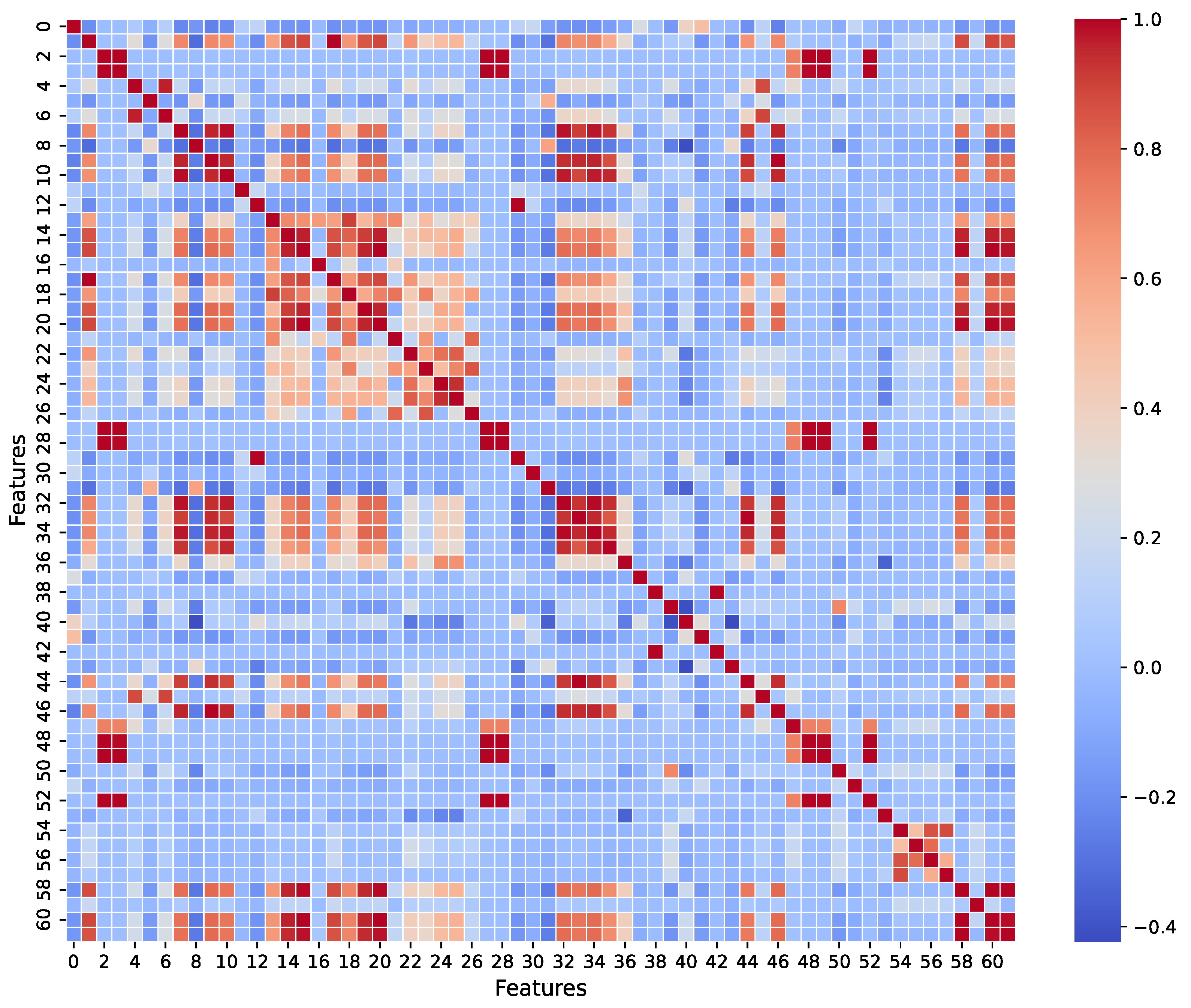
The next step in the preprocessing process involves normalising the features by subtracting their mean value and dividing by their standard deviation. Figure 1 shows the covariance matrix of the features after the preprocessing step. As seen in Figure 1, all diagonal elements of the covariance matrix represent large values that indicate the successful removal of zero variance features. Further analysis reveals similar patterns across certain features, indicating strong covariance. However, upon closer inspection, we observe that despite their high correlation, these features still exhibit subtle differences that could be critical for classification.

We refrain from further elimination at this stage to ensure that no potentially valuable discriminative information is lost. Instead, we allow the next step of the proposed approach to identify the most relevant features for the learning process.

As the final step of the preprocessing, we modify the labels. As shown in Table 1, the dataset contains six classes of samples. The class BENIGN represents normal activities, while the other five classes correspond to different types of malicious attacks. Since we aim to design an intrusion detection system, we modify the labels to fit an anomaly detection framework. Specifically, as shown in Table 1, we assign label 0 to BENIGN samples and label 1 to all other samples.

4.3. Calculating Feature Importance Scores (Step 2)

Feature importance scores quantify the contribution of each feature to a model’s predictions. These scores help identify the most relevant features, improving interpretability by reducing dimensionality (towards smaller, scoped decision trees in GlassBoost).

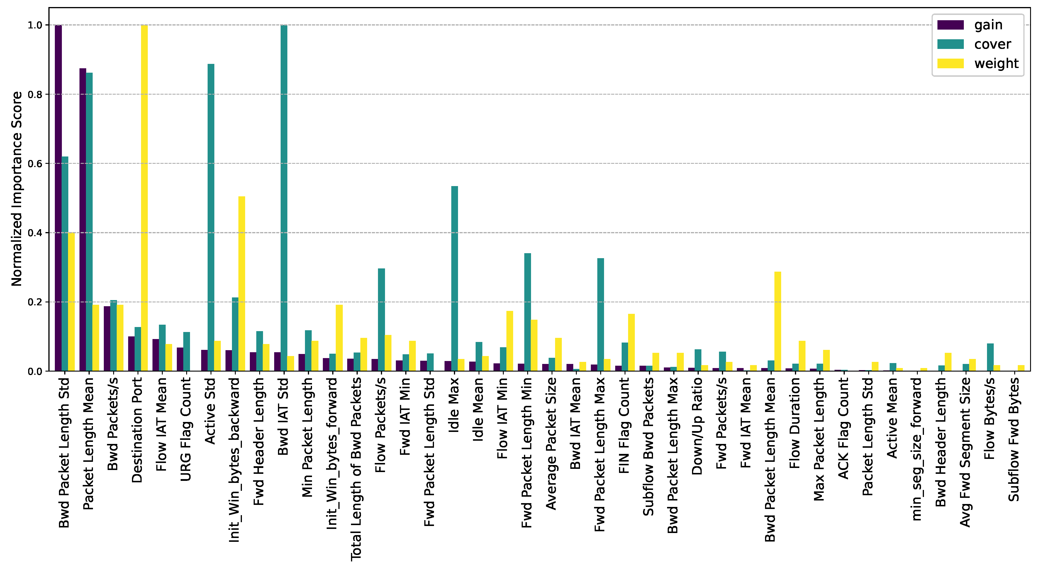
After training an XGBoost model, three feature importance scores (weight, gain, and cover) can be extracted for each feature. Weight counts how often a feature is used for splits, while cover measures the average number of samples those splits affect. The most crucial metric is the gain score, which quantifies the average improvement in the model’s objective function (e.g., loss reduction) when a feature is used for splitting. Gain is calculated as the difference in loss before and after a split, averaged across all occurrences of the feature in the boosting trees. A higher gain indicates that a feature contributes more to improving model performance.

When training an XGBoost model, every time a feature is used to split a node, the gain is computed for that split according to Equation (23). XGBoost sums the gain values across all occurrences of that feature in all boosting decision trees [31]. Readers are referred to Section 3.2 for further information on gain score calculation.

We trained the XGBoost model on the dataset using 70% of samples for training and the remaining 30% for validation. The loss function values were monitored at each boosting step during training to prevent overfitting. The training samples were selected randomly, and the maximum number of boosting trees was limited to 50. The boosting tree depth was limited to 4, and the objective function binary:logistic was used which is standard objective function for binary classification tasks [31]. Regarding the number and depth of the boosting trees, we should emphasise that our objective is not to construct a model for deployment, but rather to construct a sufficiently accurate model capable of capturing meaningful patterns in the training data without overfitting. This model is primarily used as a tool for extracting gain scores to identify important features. Based on the performance metrics obtained under this configuration, the XGBoost model has been trained effectively, demonstrating excellent results on the test dataset, with an accuracy of 0.9960, a precision of 0.9921, and a recall of 0.9970. These results indicate that the XGBoost model has been trained effectively and that the computed gain scores are reliable.

Figure 2 shows the feature importance scores: gain, weight, and cover. It is worth noting that the feature importance scores have been scaled to the range [0, 1]. Additionally, the features on the x-axis are arranged in descending order based on their gain score.

Figure 3 only presents the gain scores, while

Table 3. Top 10 features ranked by gain scores with corresponding cover and weight scores.

Feature	Gain	Cover	Weight
Bwd Packet Length Std	1.000000	0.619524	0.400000
Packet Length Mean	0.874347	0.861828	0.191304
Bwd Packets/s	0.186786	0.204659	0.191304
Destination Port	0.099629	0.127199	1.000000
Flow IAT Mean	0.092572	0.133998	0.078261
URG Flag Count	0.067601	0.112332	0.000000
Active Std	0.061287	0.886808	0.086957
Init_Win_bytes_backward	0.060260	0.212840	0.504348
Fwd Header Length	0.054233	0.115591	0.078261
Bwd IAT Std	0.054226	1.000000	0.043478

lists the top 10 most influential features based on their gain scores, corresponding weight and cover values. Since the gain scores of some features are minimal (approximately zero), the x-axes for both Figure 2 and Figure 3 were not extended to include all the features.

4.4. Model Compression (Step 3)

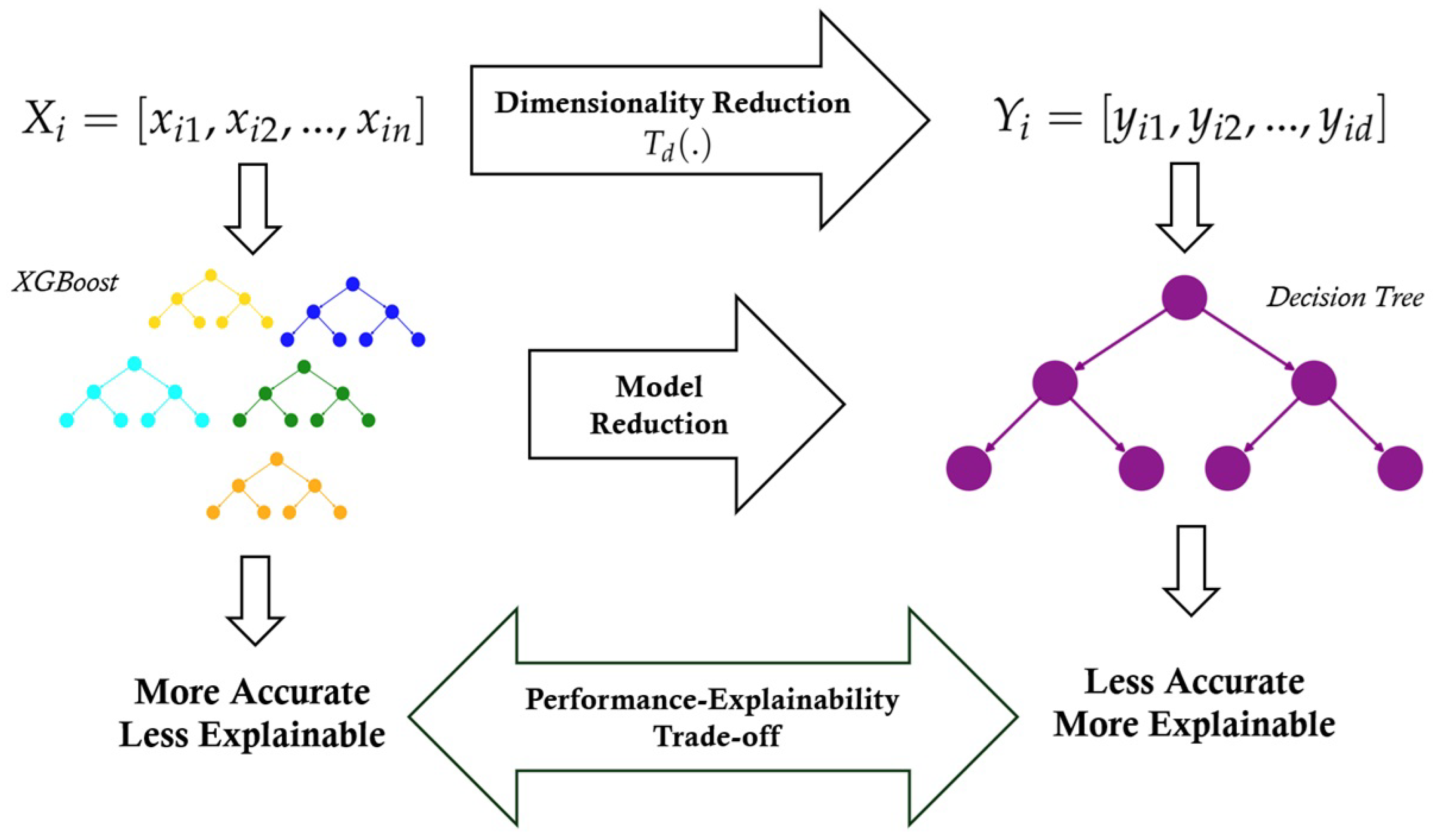
The model compression process is illustrated in Figure 4. The approach leverages gain scores to identify and select the most significant features. The selected features compress a complex XGBoost model into a simplified, more interpretable decision tree. The model compression reduces the number of contributing features and streamlines the decision-making structure, replacing a complex ensemble of multiple boosting trees with a single decision tree. Although XGBoost is highly effective in handling tabular data, its ensemble nature, consisting of multiple decision trees, makes the prediction process challenging to interpret. Therefore, instead of using an XGBoost model for classification, we use the gain scores to identify the most important features. We select the d most important features, sort them, and use them to train a decision tree.

We now provide a detailed explanation of the model compression process. Suppose that we are given a dataset of N samples where each sample $i,1<i<N$, is presented by the feature vector $X_i=[x_{i1},x_{i2},\dots ,x_{in}]$ from the original feature space and n is the number of features of the feature vector $X_i$. We define a dimensionality reduction transform $T_d(.)$ from the original feature space onto the reduced feature space so that $T_d\left(X_i\right)=Y_i$, where $Y_i=[y_{i1},y_{i2},\dots ,y_{id}]$ consists of the d features from $X_i$ with the highest gain scores sorted in descending order based on their respective gain scores. The number of features in $Y_i$ should be much smaller than that in $X_i$ ($d<<n$). We can represent a set of M feature vectors from the original dataset by the matrix $\mathbf{X}$, a matrix of M rows (samples) each containing n features. Applying $T_d(.)$ on rows of $\mathbf{X}$ yields a data matrix ${\mathbf{Y}}_d$ in the reduced feature space (see (24)) with the same number of rows (samples) but with a much smaller number of columns (features).

$$\mathbf{X}={\left[\begin{array}{c}{X}_1\\ X_2\\ ⋮\\ X_M\end{array}\right]}_{\begin{array}{c}M\times n\end{array}}\underset{\Rightarrow }{T_d(.)}{\mathbf{Y}}_d={\left[\begin{array}{c}{Y}_1\\ Y_2\\ ⋮\\ Y_M\end{array}\right]}_{\begin{array}{c}M\times d\end{array}}.$$

(24)

We can assign corresponding labels and train a simple decision tree using samples in the reduced data space. This approach yields an explainable model without significantly compromising complexity. In the next section, we present the performance of GlassBoost.

5. Results

This section evaluates GlassBoost’s performance using three different decision tree configurations. Specifically, we set the maximum depth of the trees to 3, 4, and 5 in separate experiments. As discussed later in this section, further experiments for depths greater than five or less than three are unnecessary.

To conduct the experiments, we randomly sample the original data matrix and extract 40,000 samples ($M=40,000$). For each scenario, defined by a specific maximum tree depth, we vary the number of selected features (d) from 1 to 40. For each value of d, the samples are projected onto a reduced feature space. Subsequently, 80% of the dimensionality-reduced samples are used for training, while the remaining 20% are reserved for testing. For decision tree implementation, we use the Scikit-learn package (version 1.0.2). The Gini impurity criterion is employed for node splitting. Except for the maximum depth, all other parameters remain at their default values as specified in [36].

For the first experiment, we limit the maximum depth of decision trees to 3.

Table 4. GlassBoost performance metrics (precision, recall, and accuracy) for varying numbers of selected features (maximum depth: 3).

Number of Features	Precision	Recall	Accuracy
1	0.985279	0.647099	0.868750
2	0.850094	0.934047	0.916500
3	0.948029	0.938536	0.959125
4	0.933267	0.975483	0.965875
5	0.934617	0.972376	0.965375
6	0.934617	0.972376	0.965375
7	0.932042	0.980318	0.967000
8	0.932042	0.980318	0.967000
9	0.932042	0.980318	0.967000
10	0.932042	0.980318	0.967000

presents GlassBoost’s performance metrics (precision, recall, and accuracy) versus the number of selected features.

According to Table 4, the model’s performance improves on the dimensionally reduced test set as the number of selected features increases, as expected. An interesting trade-off is observed when the number of features is increased from one to two in the decision tree model (Table 4). While the model with a single feature achieves high precision (0.9853), its recall is substantially lower (0.6471), indicating a tendency to be overly conservative. It correctly identifies positive instances when it does flag them but misses many actual intrusions. Introducing a second feature results in a marked increase in recall (to 0.9340) but with a corresponding drop in precision (to 0.8501). This suggests that the additional feature enables the model to capture a broader range of anomalies, improving sensitivity at the cost of admitting more false positives. The overall accuracy improves from 0.8688 to 0.9165, indicating a more balanced approach between true positive and true negative classifications. This trade-off highlights the impact of feature inclusion on model behaviour, particularly in scenarios where high recall is critical, such as intrusion detection.

No further improvement is observed beyond a certain point ($d>7$). This can be attributed to the structure of the decision tree. A maximum tree depth of three allows for, at most, seven splitting nodes. Consequently, any additional features beyond this threshold do not contribute to the decision-making process. In other words, these later features are not selected for the decision nodes because the earlier, more discriminative features have already been selected. 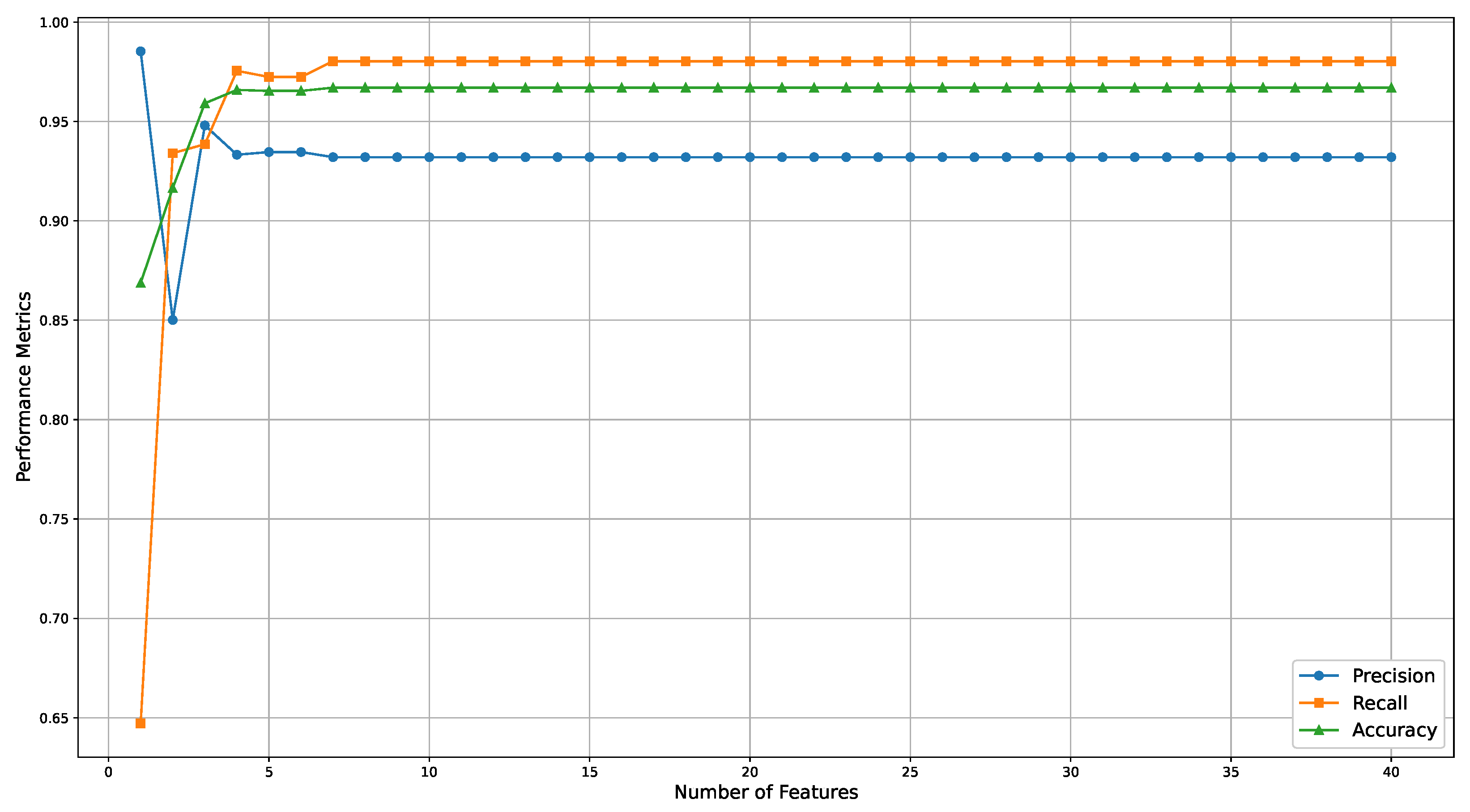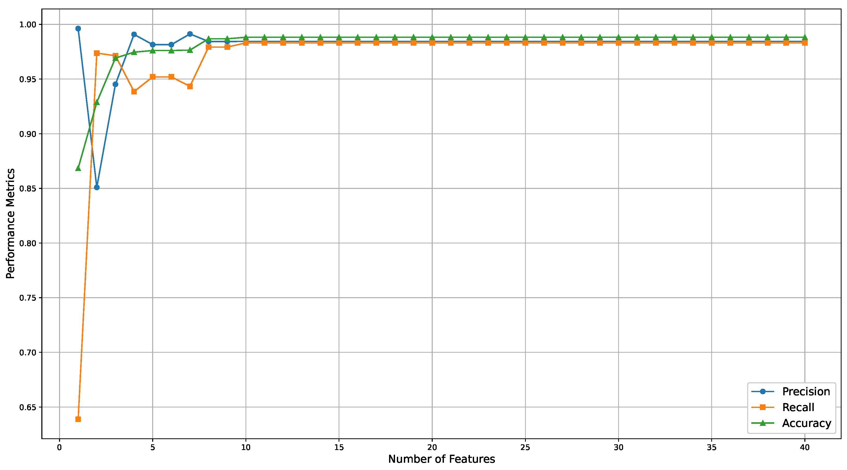Figure 5 illustrates the performance metrics for this scenario across a broader range of selected features ($1\le d\le 40$), visually representing how these metrics evolve. The results indicate that a decision tree with a maximum depth of three, using only seven features, is sufficient to create an explainable model with a precision of 0.9320, a recall of 0.9803, and an accuracy of 0.9670 (see row seven of Table 4).

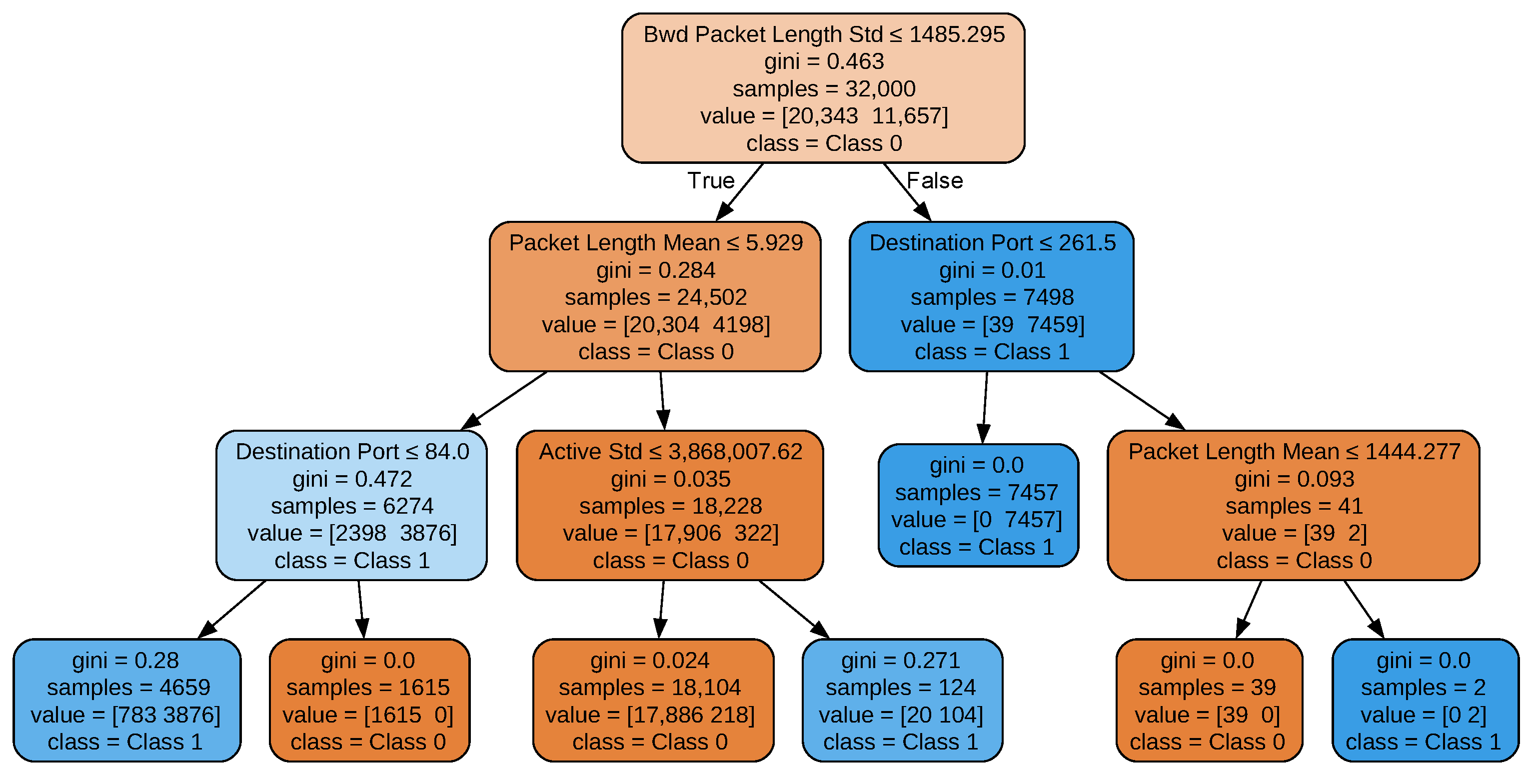
Figure 6 illustrates the tree structure of GlassBoost in this case when d = 7 and maximum depth = 3. A notable observation from Figure 6 is that not all of the seven most important features are utilised in the decision nodes, while some appear multiple times. This indicates that the decision nodes prioritise features that enhance the model’s performance on the training set. Specifically, the features Destination Port and Packet Length Mean are selected multiple times, while the feature Bwd Packets/s is not selected despite having a higher gain value than Destination Port. This suggests that certain features may not improve decision performance if they correlate with higher-ranked features already incorporated into the decision process. The same behaviour is seen when the tree depth is increased. Regarding the color scheme in the decision tree diagram, the two distinct colors represent the two classes in our binary classification task. Additionally, the brightness of each color corresponds to the Gini index at each node, with lighter shades indicating higher impurity. This color-coding approach is consistently applied across all decision tree diagrams presented in this paper.

In Figure 6, the decision tree consists of seven leaf nodes. Consequently, the tree can be represented as a rule-based classifier comprising seven classification rules, each corresponding to a single leaf node. These rules can be expressed in the form of IF–THEN statements. For example, Equations (25)–(28) illustrate the rules derived from the leftmost leaf of the tree.

$$\mathrm{IF}\mathrm{Bwd}\mathrm{Packet}\mathrm{Length}\mathrm{Std}\le 1485.295,$$

(25)

$$\mathrm{AND}\mathrm{Packet}\mathrm{Length}\mathrm{Mean}\le 5.929,$$

(26)

$$\mathrm{AND}\mathrm{Destination}\mathrm{Port}\le 84,$$

(27)

$$\mathrm{THEN}\mathrm{Anomaly}\mathrm{Class}(\mathrm{Class}1).$$

(28)

For the next scenario, we limit the maximum depth of the decision trees to four and repeat the same procedure. Figure 7 presents the performance metrics as a function of the number of features for this case.

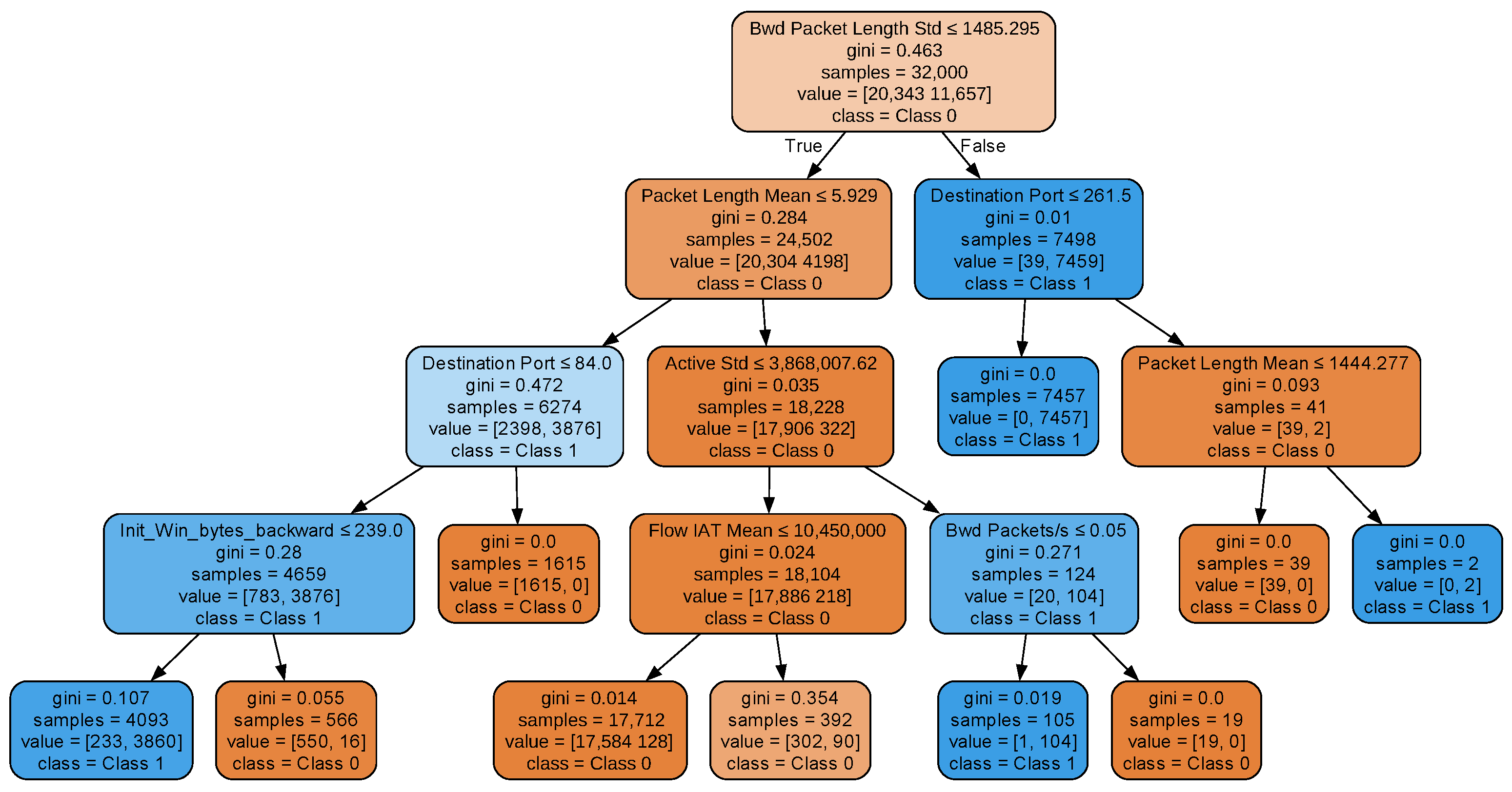
As depicted in Figure 7, utilising a decision tree with a maximum depth of four leads to a substantial improvement in model performance compared to the model with a maximum depth of three. Specifically, by incorporating the eight most influential features, the model achieves a precision of 0.9843, a recall of 0.9792, and an accuracy of 0.9868. Similar to the previous analysis, increasing the number of features beyond a certain threshold does not improve performance (in this case, beyond eight). The resulting decision tree for this case (d = 8, maximum depth = 4) is illustrated in Figure 8.

As shown in Figure 8, the resulting decision tree has ten leaf nodes, implying that an equivalent rule-based classifier would require ten IF–THEN statements. So, increasing the decision tree depth enhances performance but compromises explainability. However, in terms of explaining individual decisions, that increase is marginal. Specifically, for the three-depth tree, six decision states (leaf nodes) have three predicates in their IF–THEN statements, and one decision state has two. Here, six decision states have four predicates in their IF–THEN statements, three have three predicates, and one has two predicates.

As the final configuration, an additional experiment is conducted with the maximum tree depth set to five. The performance metrics from this experiment, along with those from the previous configurations (maximum depths of three and four), are summarised in the first three sections of

Table 5. GlassBoost performance comparison with different maximum depths and SHAP.

		Number of Features
		1	2	3	4	5	6	7	8	9
GlassBoost (Maximum depth = 3)	Precision	0.9852	0.8500	0.9480	0.9332	0.9346	0.9723	0.9346	0.9320	0.9320
	Recall	0.6470	0.9340	0.9385	0.9754	0.9723	0.9803	0.9803	0.9803	0.9803
	Accuracy	0.8687	0.9165	0.9591	0.9658	0.9653	0.9653	0.9670	0.9670	0.9670
GlassBoost (Maximum Depth = 4)	Precision	0.9962	0.8509	0.9452	0.9908	0.9814	0.9814	0.9912	0.9843	0.9843
	Recall	0.6388	0.9737	0.9713	0.9385	0.9520	0.9520	0.9433	0.9792	0.9792
	Accuracy	0.8683	0.9287	0.9692	0.9746	0.9761	0.9761	0.9765	0.9868	0.9868
GlassBoost (Maximum Depth = 5)	Precision	0.9941	0.8514	0.9489	0.9922	0.9899	0.9899	0.9869	0.9865	0.9865
	Recall	0.6481	0.9737	0.9696	0.9723	0.9896	0.9896	0.9886	0.9899	0.9899
	Accuracy	0.8712	0.9290	0.9701	0.9872	0.9926	0.9926	0.9911	0.9915	0.9915
SHAP tree (Maximum depth = 4)	Precision	0.9853	0.8419	0.9333	0.9333	0.9333	0.9333	0.9333	0.9346	0.9346
	Recall	0.6471	1.0000	0.9755	0.9755	0.9755	0.9755	0.9755	0.9724	0.9724
	Accuracy	0.8688	0.9320	0.9659	0.9659	0.9659	0.9659	0.9659	0.9654	0.9654

.

A similar trend is observed when the maximum depth is increased to five: performance metrics show no significant improvement beyond including eight features. Moreover, extending the depth from four to five results in only marginal performance gains.

The resulting decision tree, with a maximum depth of five, contains 15 leaf nodes, translating to 15 sets of IF–THEN rules in an equivalent rule-based classifier (see Figure 9). However, the performance improvement compared to a decision tree with a maximum depth of four is minimal. Therefore, if explainability is a primary concern, increasing the model’s complexity may not be justified for such a slight performance gain. Nonetheless, depending on the specific application and user needs, even a slight enhancement in accuracy might be worthwhile when performance is prioritised over explainability.

Investigating the three decision trees reveals the following facts. Each tree begins by evaluating the feature Bwd Packet Length Std with the initial question: “Is Bwd Packet Length Std less than or equal to 1485.295?” at the root node. This feature was identified as the most critical for classifying network traffic due to its highest gain score (see Section 4.3). The Gini impurity score for this node is 0.463, indicating the degree of class mixture: a lower Gini score signifies better class separation. The root node contains 32,000 samples (the total training samples), with a distribution of [20,343 11,657]. This means 20,343 samples belong to ‘Class 0’ (normal traffic), and 11,657 samples belong to ‘Class 1’ (anomalous traffic). The term class = Class 0 denotes the majority class at this node. The root node branches based on whether the condition (Bwd Packet Length Std ≤ 1485.295) is true or false. Following the ‘True’ branch indicates the condition is met while following the ‘False’ branch indicates it is not. Each internal node poses additional questions about other features. For instance, at the next level (depth 1) in all three trees, the features Packet Length Mean and Destination Port are evaluated. This process continues until the tree reaches its maximum allowed depth.

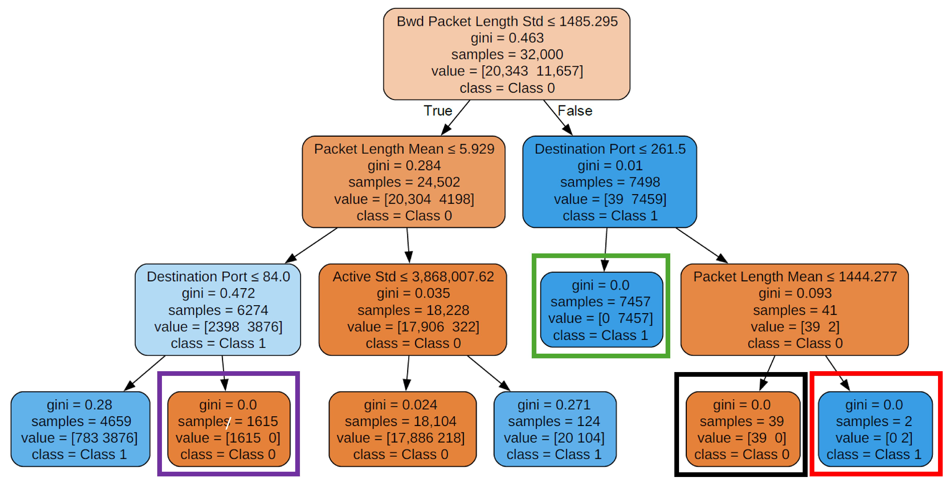
In Figure 10, four nodes in the depth-three decision tree are outlined with rectangles in purple, black, green and red. These nodes exhibit notable properties. First, their Gini scores are zero, indicating that these nodes are pure, containing samples from only one class. Second, as the decision tree grows deeper, these nodes remain unchanged. This suggests that they correspond to simple yet highly discriminative rules based on a few key features, effectively classifying their target classes without being influenced by further tree expansion. These nodes represent distinct and easily interpretable patterns in the data that can be expressed as a set of IF–THEN rules. For example, the node highlighted by a green rectangle can be described by the following simple rule:

IF Bwd Packet Length Std > 1485.295 and Destination Port $\le 261.5$, THEN predicted class is ‘Class 1’.

The primary reason behind this stability is how features are selected and ordered during tree construction. Features are sorted based on their gain scores, allowing the decision tree algorithm to prioritise the most important features for splitting. Since these highly discriminative nodes emerge early in the tree and effectively separate data points, they remain unchanged as the tree deepens. Subsequent tree levels focus on identifying more complex patterns that require further refinement, rather than altering these well-established decision rules.

It is also observed that as the tree’s maximum depth increases, the number of leaves with a Gini score equal to or close to zero tends to rise. This is expected, as deeper trees can capture more complex relationships within the data. However, while increasing the depth may improve accuracy, it comes at the cost of reduced interpretability. Furthermore, a deeper tree is more prone to overfitting, making it overly sensitive to specific patterns in the training data and diminishing its ability to generalise to unseen samples.

Although increasing the maximum depth to five yielded no substantial performance gains over a depth of four, using a depth of three resulted in lower accuracy but improved explainability. A depth of four, therefore, appears to offer a good balance between performance and interpretability. We should emphasise that while the interpretability of the model structure is preserved, as the output remains in the form of IF–THEN rules, comprehensibility may diminish as the number of rules increases. In such cases, although the model is still technically interpretable, it may become more challenging for users to extract clear insights.

To better highlight the performance of GlassBoost, we compared it with the well-established SHAP method. To this end, we applied SHAP to the baseline XGBoost model introduced in Section 4.3. Figure 11 presents the resulting SHAP summary plot for the 10 top important features according to SHAP analysis. This plot visualises feature importance and its impact on the baseline XGBoost output. The y-axis lists features sorted from top to bottom by their global importance, which is calculated as the average absolute SHAP value across all data instances for that feature. The x-axis displays SHAP values, indicating a positive (right) or negative (left) influence on the prediction. The colour bar (red for high and blue for low) reveals the correlation between the original feature value and its impact, with each dot representing a data instance.

To ensure a fair comparison, we evaluated the performance of decision trees trained on features selected by GlassBoost against those trained on features identified using the SHAP method. As noted earlier, the first three sections of Table 5 present the performance metrics for decision trees based on GlassBoost-selected features. The final section of the table summarises the performance of decision trees trained on SHAP-selected features. Henceforth, we will refer to those latter decision trees as SHAP trees. We set the maximum depth of the SHAP trees to four, allowing for a fair comparison to similar-depth trees generated by GlassBoost.

Compared to SHAP trees, GlassBoost demonstrates superior and more balanced performance across all three evaluation metrics: precision, recall, and accuracy. While SHAP trees achieve a recall of 1.0 with just two features, this comes at the cost of significantly lower precision (0.84) and only moderate accuracy (0.932), indicating a higher rate of false positives. Moreover, the performance of SHAP trees stagnates in the range of three to seven features, with minimal improvements across all metrics, suggesting that it may not effectively identify informative features. In contrast, GlassBoost continues to improve as more features are added, steadily enhancing all three metrics. This indicates that GlassBoost is more successful at selecting a compact yet informative set of features. Notably, as the number of features increases, GlassBoost begins to outperform SHAP across the board, achieving higher recall while also maintaining significantly better precision and accuracy. These results make GlassBoost a more robust and practical choice, especially in domains where both performance and explainability are critical.

To conclude this section, it is essential to note that exploring the performance of GlassBoost with shallower or deeper structures is unnecessary due to the bias–complexity trade-off. A tree with a depth of one relies on a single feature for its prediction, which is referred to as a decision stump. A decision tree with one internal node (the root) is immediately connected to the leaf nodes. A decision stump makes a prediction based on the value of just a single feature. A two-depth tree can incorporate three features at most. In either case, such shallow models are highly biased and cannot capture nuanced patterns in the data, resulting in poor predictive performance.

On the other hand, we previously observed that increasing the tree depth from four to five does not significantly improve performance. Similarly, extending the depth beyond five offers no substantial gains. This is evident from the Gini indices of the leaf nodes in a five-depth tree, where most values are close to zero, indicating high purity. Further increasing the depth would likely lead to overfitting, as the model would memorise the training data rather than generalise to new data.

6. Discussion

This study introduced a novel, explainable model that can be applied to tabular data in general, with its effectiveness demonstrated through a case study in intrusion detection. This section focuses on its empirical impact and broader implications. GlassBoost compresses a high-performing XGBoost model into a simpler decision tree that retains most of its predictive power while providing interpretability through transparent IF–THEN rules.

As discussed in Section 4.3, the original XGBoost model trained on 62 input features achieved outstanding performance (accuracy: 0.9960, precision: 0.9921, and recall: 0.9970) using 50 boosting rounds and a maximum depth of four per tree. However, this model is inherently complex and difficult to interpret, both due to its size and the ensemble nature of boosted trees.

To address this, we utilised the gain scores from XGBoost to rank feature importance and selected the top d features for training a set of decision trees. This technique enables model simplification while maintaining performance, making it suitable for constrained or transparency-critical environments. For instance, a decision tree with a maximum depth of four using just eight features yielded an accuracy of 0.9835, outperforming many XAI models reported in [37] (see

Table 6. Comparison of the accuracy of GlassBoost with XAI models introduced in [37].

XAI Model	Accuracy
GlassBoost (maximum depth = 4, $\mathit{d}$ = 8)	0.9835
Random Forest	0.9852
Gradient Boosting	0.9907
Rule-based	0.9728
KNN	0.9785
Linear regression	0.9635
SVM	0.9868
Adaboost	0.9889
XGBoost	0.9905

). Only AdaBoost, XGBoost, and gradient boosting achieved higher accuracy but with fewer transparent model structures. However, other metrics, such as precision and recall, were not reported in [37], and the authors’ exact definition of gradient boosting is unclear. For those techniques where the decision tree of depth four was less accurate, the preliminary XGBoost model, used to extract the gain values, provided better accuracy. Moreover, the number of features used in [37] was 15, while the decision tree of depth 4 uses only 8 features.

A more detailed comparison with the models in [23], who also used the same dataset and identified their top features via SHAP, is presented in

Table 7. Comparison of GlassBoost with XAI-IDS [23].

Model	Accuracy	Precision	Recall
GlassBoost (maximum depth = 4, $\mathit{d}$ = 8)	0.9868	0.9843	0.9792
Random Forest	0.99	0.96	0.96
AdaBoost	0.93	0.78	0.78
Deep Neural Network (DNN)	0.94	0.80	0.80
Support Vector Machine (SVM)	0.99	0.97	0.97
K-Nearest Neighbor (KNN)	0.99	0.99	0.99
Multi-Layer Perceptron (MLP)	0.96	0.88	0.88
LightGBM	0.97	0.92	0.92

. Our GlassBoost model (depth four, d = 8) achieved high scores across all key metrics (accuracy (0.9868), precision (0.9843), and recall (0.9792)), comparing favourably to state-of-the-art models, including random forest, SVM, and KNN. While the accuracy of these models was marginally higher (0.99), our approach provides explainability with minimal sacrifice in predictive performance. It also demonstrates robustness across key metrics, suggesting suitability for operational use where both precision and recall are critical. Moreover, it outperformed more complex methods such as DNN and MLP in all three metrics.

GlassBoost’s advantage lies not only in its competitive performance but also in its simplicity. Unlike black-box models that rely on post hoc interpretability tools, our approach is inherently explainable, providing direct insight into the decision logic. This is especially valuable in domains where transparency, auditability, and user trust are paramount, such as security-critical or regulated environments.

An additional strength of GlassBoost is its computational efficiency. With low memory and processing requirements, it offers a reliable and effective solution for edge computing [38]. In this context, smart edge devices are deployed at the network’s edge, close to mobile devices or sensors, where computational resources are often limited. In such scenarios, implementing a fast, accurate, and explainable model is crucial for the early detection of anomalies. To support this claim, we refer readers to [29], which demonstrates that when a CART tree is grown to a uniform depth of D, i.e., to $2^D$ terminal nodes, the sorting time is proportional to $N(D+1)({log}_{2}N-{\displaystyle \frac{D}{2}})$, and the evaluation time is proportional to $N(D+1)$, where N is the number of features. Our approach significantly reduces the number of input features: for example, in the CyberSecurity dataset, we reduced 62 features to at most 8 while maintaining strong performance using a decision tree of depth 4. Based on this empirical evidence and the theoretical facts from [29], we assert that GlassBoost qualifies as a lightweight and efficient model well-suited for resource-constrained environments. It is also worth noting that the training phase, although computationally more intensive, is performed only once. Subsequently, the evaluation of new samples is highly efficient, as the resulting model is a shallow decision tree with minimal inference overhead.

Additionally, GlassBoost can quickly adapt to data or concept drift as long as these shifts do not substantially alter the set of important features. However, if the underlying data distribution changes to the extent that the key features lose their relevance, a new feature set must be identified. This can be accomplished by reapplying XGBoost to updated datasets that capture evolving data patterns.

Finally, GlassBoost can be applied to many datasets, provided they include tabular data. While this study focused on intrusion detection, the approach broadly applies to any classification or detection task where a balance between explainability and performance is desired. It is particularly well-suited to domains that require interpretable decision-making pipelines, such as healthcare, finance, and IoT, where insight into model behaviour is as important as accuracy. Moreover, unlike most methods that only quantify the contribution of each feature to the model’s final decision, GlassBoost goes a step further. It determines feature importance and provides a transparent, rule-based explanation of the entire model using simple IF–THEN rules, enhancing interpretability and trustworthiness.

7. Conclusions

This study introduced a novel explainable artificial intelligence (XAI) framework for the intrusion detection problem. It combined the capabilities of XGBoost in generating importance scores, specifically gain, to select the most important features. The selected features were utilised to generate decision tree classifiers that were both accurate and interpretable. GlassBoost achieves strong performance and model transparency, offering a practical alternative to complex black-box models. Its simplicity and low computational requirements make it well-suited for deployment in resource-constrained environments such as edge computing systems.

Although the method demonstrates competitive performance on standard machine learning problems focused on tabular data, it inherits certain limitations from its underlying tree-based models. In particular, tree-based models, such as decision trees and gradient-boosting machines (GBMs), do not inherently capture temporal dependencies, which can be critical in time-series data that exhibits trends or seasonal variations. Consequently, the framework may be less effective in domains with a dominant temporal structure.

Furthermore, simplifying a model to enhance its transparency often comes at the cost of reduced predictive performance. However, a model’s performance is also heavily dependent on the nature of the data it is trained on, as emphasised by the no free lunch theorem. In our approach, the baseline model is XGBoost, from which we identify the most informative and discriminative features using gain scores obtained during training. When a small subset of features accounts for the majority of the cumulative gain score, it suggests that model compression (smaller trees of smaller depth) can preserve most of the original predictive power and yield results comparable to those of the complete baseline model. Nevertheless, some loss in performance is still expected due to simplification.

Future work should focus on applying the framework to similar problems/exploring its applicability across a broader range of anomaly detection and classification tasks. Furthermore, extending XGBoost to multi-class problems is indeed feasible. GlassBoost can be readily extended to multi-class classification tasks by training the baseline XGBoost model on a multi-class dataset. The gain scores used in our feature selection process are computed in the same way, and the subsequent model compression step remains straightforward. Since decision trees are inherently capable of handling multi-class problems, this extension aligns naturally with our approach.