Time Scale Control Using Dynamic GMDH Neural Network Forecasting Based on Real Measurement Data

Abstract

This article presents the results of the conducted research work related to the dynamic forecasting of the difference values for the Polish Time Scale UTC(PL) for real measurement data, prepared in the form of the time series TS1 and TS2. For the presented time period (the whole year of 2024), the differences between the UTC(PL) and UTC does not exceed ±4.4 ns. The analogous differences for the interval exceeding 2 years are within the range of ±5 ns. Additionally, the obtained forecast results for the last day of forecasting in a given week are very consistent with the forecast results for the first day of the new forecasting week, which illustrates the very good quality of the forecasting and the universality of the forecasting procedure developed by the author using the GMDH-type neural network.

1. Introduction

In the rapidly developing world of technology, the adaptability and flexibility of systems become crucial to achieving optimal efficiency and effectiveness. Some of the fundamental aspects of system control are managing the pace and continuity of operation, which are mainly responsible for time scales steering. Traditional methods of controlling time scales are often based on predefined rules or simple feedback loops. However, in complex and unpredictable environments, these methods may prove to be insufficient.

Time scale control is required to ensure precise synchronization of the atomic clock implementing this scale with the UTC coordinated universal time [1]. National UTC(k) time scales are the basis for determining the official time in a given country, and are implemented by the leading National Metrology Institutes (NMIs). National NMIs strive to ensure the best possible stability and accuracy of their UTC(k). For this purpose, a direct comparison of a given UTC(k) with the global UTC scale, determined by the International Bureau of Weights and Measures, BIPM (in French, Bureau International des Poids et Mesures) is required [2,3,4]. This is mainly related to the need for the NMI to have a frequency that has high accuracy and stability, and also the possibility of its precise synchronization. This, in turn, very often is the basis for the safety and quality of many systems and for conducting basic scientific research. Currently, very important and advanced work is being carried out on the future definition of a second, according to the SI system, and on the revision of the definition of the international coordinated universal time, UTC.

Every month and every week, for an individual UTC(k), the BIPM determines the UTC–UTC(k) and UTCr–UTC(k) differences, respectively. The UTC–UTC(k) differences define the divergence of national time scales in relation to the UTC, while the UTCr–UTC(k) differences define the divergence in relation to the UTC Rapid scale [5]. The UTC–UTC(k) differences for the previous month are published in the “Circular T” bulletin on MJD (Modified Julian Date) days ending with 4 and 9 (with a 5-day interval), most often in the second decade of the following month, while the UTCr–UTC(k) differences for the previous week are published every Wednesday at 7:00 p.m. on the BIPM FTP server.

Delays in the publication of the UTC–UTC(k) and UTCr–UTC(k) differences by the BIPM cause difficulties in maintaining the highest possible level of compliance of the UTC(k) with the UTC. The main factor that influences this situation is the time needed to collect, properly prepare, and verify the measurement data from local and remote comparisons of over 700 atomic clocks [6], sent to the BIPM by the NMI, Designated Institutes, and other laboratories that are responsible for the implementation of local UTC(k) time scales, as well as the high complexity and time-consuming process of calculating the UTC scale by the BIPM [1,2].

In view of the problem of the delay in the publication of the differences determined by the BIPM, the control and determination of national UTC(k) time scales are based, in most cases, on forecasting methods (time or frequency scale). Statistical methods are used for this purpose, namely linear regression [7], Allan deviations [8], a Kalman filter [9], or stochastic differential equations [10]. In many cases, these methods are often combined with a heuristic decision-making process [7,11,12]. The availability of a local primary or secondary frequency standard (PFS or SFS) provided by the NMI, i.e., a caesium fountain, rubidium fountain, or optical clock [11], only allows for changing the time horizon of forecasts, or it may be more important in the case of a period of unavailability of PFS/SFS signals [6,11,12]. Forecasting has a significant impact on ensuring the greatest possible compliance of the UTC(k) with the UTC. Furthermore, ensuring the best possible compliance provides a reliable source of measurement traceability in regard to the time and frequency domains for the UTC(k) scale, as well as the possibility of precise synchronization and independence from less reliable external sources.

In recent years, neural networks, inspired by the human brain, have revolutionized many fields of science and engineering, from image and speech recognition to natural language processing. Their ability to learn complex relationships from data and adapt to changing conditions opens up new possibilities for intelligent control. In this context, the application of neural networks for the dynamic control or forecasting of the national time scale, UTC(k), has become a promising direction of research and development.

The Polish Time Scale UTC(PL) is implemented by the Time and Length Department of the Central Office of Measures (GUM) in Warsaw, using the active hydrogen maser VCH-1003M. Until 2016, UTC(PL) forecasting was performed based on the aforementioned statistical method of linear regression. At the same time, research has been conducted at the Institute of Metrology, Electronics and Computer Science at the University of Zielona Góra (IMEI UZ) on the application of various types of neural networks to forecast the Polish Time Scale. The possibility of using neural networks for forecasting results from their properties. Neural networks are a very good mathematical tool to solve very complex non-linear problems [13]. The main goal of these research works was to obtain a better quality of UTC(PL) forecasting in relation to the previously used linear regression method [14,15,16]. The research results presented in these works, based on historical data, showed the possibility of achieving a significantly better quality of UTC(PL) forecasting using the GMDH (group method of data handling) neural network [17], in comparison to other methods that were compared using the same input data. The results of the research clearly showed that the GMDH neural network has the best forecasting properties [18]. GMDH neural networks are an innovative category of self-organizing networks. Their key feature is the use of the group method of data handling, which is widely used in various areas, such as data acquisition, prediction, the modelling of complex systems, and process optimization [17]. They have the ability to automatically optimize the networks during the training process. This includes the precise adjustment of the number of hidden layers and the number of neurons in each of these layers. The activation functions that drive the neurons in these networks most often take the form of polynomials, which allows for the effective modelling of non-linear dependencies in the data. In addition, the good forecasting properties of the GMDH-type neural networks enable the quick adaptation of these neural networks to the nature of the data used as input.

As a result of the conducted research work, a procedure for forecasting the national UTC(k) time scale has been developed using a GMDH-type neural network [19]. First, the correctness of the developed procedure has been verified for time scales implemented based on commercial caesium atomic clocks, hydrogen masers, and hydrogen masers supervised by the primary frequency standard in the form of a caesium fountain [20,21]. The research results presented in the cited publications showed that the developed procedure is universal and enables the achievement of very good quality UTC(PL) forecasting [22], as well as other national UTC(k) time scales. This has resulted in a forecasting procedure based on a GMDH-type neural network being used to control the Polish Time Scale UTC(PL) by the Time and Length Department of the Central Office of Measures, since 2016, which enables the dynamic forecasting of the UTC(PL) based on real measurement data.

The aim of this work is to show the potential of neural networks as a powerful tool for creating more intelligent, flexible, and effective systems, using them as an example for time scale control. This work presents the findings from the conducted research, showing the weekly forecasting results for the Polish Time Scale UTC(PL) using a GMDH-type neural network, based on real measurement data on the phase time, realizing the UTC(PL) time scale for the GUM and the values of the UTCr–UTC(PL) differences. This work presents the results of the forecasting differences for the UTC(PL), with a 1-day interval for the entire upcoming week (from Wednesday to the following Wednesday). For this purpose, a GMDH-type neural network is used, with the developed procedure [19], for real data prepared in the form of two time series, TS1 and TS2, built on the basis of the differences determined according to the UTC and UTC Rapid scales. This article is of a practical nature, it focuses on the presentation of the entire process of conducting research related to the dynamic forecasting of the UTC(PL) based on real measurement data, which has been implemented by the GUM and is used for the current control of the UTC(PL). The forecasts for 2024, presented in the article, have been used by the GUM to control the Polish Time Scale UTC(PL).

2. Materials and Methods

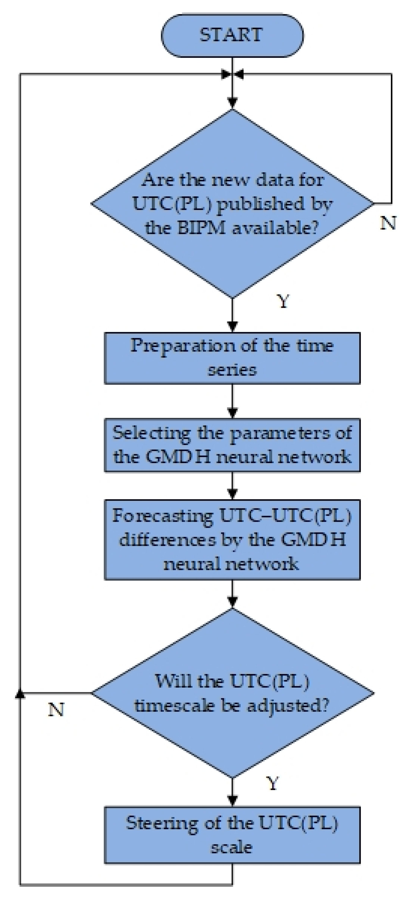
The research related to the weekly forecasting of the Polish Time Scale UTC(PL) using a GMDH-type neural network, based on actual measurement data, is carried out based on the developed forecasting procedure. A block diagram presenting the operation of the forecasting procedure is presented in Figure 1. The procedure begins with checking whether the BIPM has published new UTC–UTC(PL) or UTCr–UTC(PL) data on the FTP server. When new data is found, an appropriate time series is prepared, taking into account this data. The next step is to train the GMDH-type neural network based on the appropriately prepared input data. The selected parameters of the neural network play a key role in the training process. Empirical studies conducted by the author indicated that the greatest impact on the quality of training concerns the selection of the degree of the polynomial activation function of the neuron and the appropriate selection of the ratio of training to testing data. The validation criterion was the option of including the entire data set in the testing process of the GMDH neural network. After the appropriate selection of the parameters, guaranteeing that the smallest value of errors are encountered during the training process, the UTC–UTC(PL) difference values are forecast for the entire upcoming week, the forecast results are sent to the GUM, and the forecasts are included in the process of controlling the Polish Time Scale UTC(PL).

One of the most important aspects of dynamic time scale forecasting is the proper preparation of the input data for the GMDH-type neural network. This is the main element of the developed forecasting system, based on the forecasting procedure. The use of a method that allows for the proper preparation of these data, in the form of an appropriate time series, has a very strong impact on the quality of the obtained forecasts. For the purposes of conducting research related to the dynamic forecasting of the Polish Time Scale UTC(PL) based on real measurement data, two time series (TS1 and TS2) have been developed, containing data with a 1-day interval.

The TS1 time series preparation method assumes the use of three types of data: the phase time values xa(t) between the 1 pps (pulse per second) signals from the UTCPL(t) and the atomic clock implementing this scale (clock_PL), the xb(t) values, which represent the UTC–UTC(k) difference values, and the xbr(t) values, which represent the UTCr–UTC(k) difference values, determined according to the following relationships:

xa(t) = UTC_PL(t) − clock_PL(t),

(1)

xb(t) = UTC(t) − UTC_PL(t),

(2)

xbr(t) = UTCr(t) − UTC_PL(t).

(3)

The values of xb(t) described by the above relationship (2) are based on the differences published in the bulletin “Circular T” by the BIPM for the UTC(PL) for the MJD days ending with 4 and 9, i.e., with a 5-day interval. In order to determine the values of these differences for each day, the Hermite polynomial interpolation, available in all versions of MATLAB since 2017 (PCHIP function), is used. Thanks to this function, the number of training data is extended, which provided the required minimum number of input data for the GMDH-type neural network. A failure to provide the required minimum number of training data may adversely affect the process of training the GMDH-type neural network [15]. Determining the data with a 1-day interval also shortened the time period for the input data, which is also of great importance in regard to forecasting the UTC(k) in the case of a clock replacement. The values of the xbr(t) differences described by relationship (3) are the data determined by the BIPM based on the UTC Rapid scale and that are published every Wednesday at 7:00 p.m. on the FTP server.

In order to prepare the final training data for the GMDH-type neural network, the appropriately prepared time series that is used as the input into the GMDH-type neural network is composed of two data subsets. The first one, x₁(t), contains data groups (from 1 to i) from day t₀ to day t_n, which is determined according to the relationship:

x₁(t) = xa(t) + xb(t) = UTC(t) − clock_PL(t).

(4)

Day t_n is the day for which the last value of this time series is known before the date of each publication of the “Circular T” bulletin (t_pub).

In turn, the second subset, x₂(t), is the supplementation of the TS1 time series with the group of data between days t_n and t_nr, which is determined according to the relationship:

x₂(t) = xa(t) + xbr(t) = UTCr(t) − clock_PL(t).

(5)

The differences in regard to xbr(i) are published every Wednesday on day t_pubr. This is also the first possible day of the forecast (t_forecast). Every week, after the publication of new values of the xbr(t), the time series TS1 data are supplemented with new data calculated based on (5). At the time of publication of a new bulletin “Circular T”, the new data i + 1 are determined based on relationship (4), which for the appropriate days replace the previous data determined based on relationship (5).

The method of preparing the TS2 time series is very similar to the preparation of the TS1 series. The only difference is that the first group of data consists only of the values of the xb(t) differences supplemented with the missing values determined by the PCHIP function. The second group of data consists of the xbr(t) difference values only.

The general method of preparing the TS1 and TS2 time series is presented in Figure 2. A detailed description of the preparation of the TS1 and TS2 time series is presented in [19,22].

The dynamic forecasting of the Polish Time Scale UTC(PL), using actual measurement data, for the Time and Length Department of the GUM, by the IMEI UZ, is conducted every Wednesday, after the publication of the xbr(t) data by the BIPM, with a 1-day interval for the entire upcoming week (from Wednesday to the following Wednesday). For this purpose, a GMDH-type neural network is used, alongside the GMDH Shell tool, using a previously developed procedure. The first forecast is performed on Wednesday, with a forecast horizon of 3 days. Forecasting is performed for 8 days from the current Wednesday to the following Wednesday. The adoption of such research methodology is based on the fact that the publication of the xbr(t) data takes place on Wednesday at 19:00. Such a forecasting method has been adopted so that the employees of the Time and Length Department in the Central Office of Measurements can introduce a correction to the UTC(PL) time scale control system on Wednesdays, before the publication of the xbr(t) data.

The process of conducting research related to forecasting the values of differences in the xb(t) for the UTC(PL), based on the forecasting procedure, has been described at the beginning of the chapter. In regard to the process of training a GMDH-type neural network, the key factor influencing the quality of the training process is the appropriate selection of the parameters: the ratio of training to testing data, the neuron transition function, and the validation function. The ratio of training to testing data is assumed to be in the range of 70/30 to 80/20, which guarantee the smallest values of training errors to be achieved. In the case of a GMDH-type neural network, the neuron transition function takes the form of a polynomial, the degree of which can be changed. It has been empirically verified that changing the degree of the polynomial from a linear function, through the use of a polynomial, to a quadratic polynomial enables the smallest values of training errors to be achieved. Furthermore, it has been assumed as a validation function that the entire set of input data will be used to test the current topology of the GMDH-type neural network. The process of training the GMDH-type neural network is repeated every week after the publication of new xbr(t) data by the BIPM for the combination of the three discussed parameters for the two prepared time series. Depending on the selection of the neuron’s transition function, the network structure consists of one hidden layer and several neurons in this layer (for the neuron’s transition function in the form of a linear function), several hidden layers, and a total of several dozen neurons in these layers for the neuron’s transition function in the form of a quadratic polynomial. An additional procedure affecting the speed of training and in order to achieve relatively small topology sizes is data pre-processing, which consists of determining the differences between neighboring data, and operations using trigonometric functions applied to these data.

The input data prepared using an appropriate method (TS1 time series or TS2 time series) is entered into the GMDH-type neural network. Depending on the time series of the input of the GDMH-type neural network, the value of the difference in the xb(t) is forecasted. When the data prepared in the form of the TS1 time series is fed as input into the GMDH-type neural network, the forecast for this series is obtained at the output of the GMDH-type neural network (x_1p(t_forecast)). After taking into account the value of xa(t) measured on the day of the forecast calculation, i.e., the phase time value of the clock implementing the UTC(PL) scale, the difference forecast xbf(t_forecast) is calculated according to the relationship:

xbf(t_forecast) = x₁(t_forecast) − xa(t_forecast).

(6)

In the case of input into the GMDH-type neural network prepared in the form of a TS2 time series, the obtained forecast value is simultaneously the forecasted value of the difference in regard to xbf(t_forecast). The obtained forecast values for xbf(t_forecast) can be the basis for the correction and dynamic control of the Polish Time Scale UTC(PL).

After the forecasting process is complete for the entire upcoming week (from Wednesday to the following Wednesday), the forecast results are sent by e-mail to the management and employees of the Time and Length Department at the GUM responsible for controlling the UTC(PL) time scale. Based on the received forecasts, the employee of the Time and Length Department at the GUM decides whether the time scale requires a correction in regard to the femtostepper. An example e-mail message in Polish, with forecasts determined using a GMDH-type neural network for input data prepared on the basis of the TS1 and TS2 time series for the UTC(PL) for the period from 18 September 2024 to 25 September 2024, sent to the GUM on September 18 at 7:40 p.m., is presented in Figure 3.

The time of sending the message to the GUM is representative of the very efficient process carried out in terms of the author’s work on the dynamic forecasting of the Polish Time Scale UTC(PL), using real measurement data. Performing the activities related to the appropriate preparation of the input data for the GMDH-type neural network in the form of the TS1 and TS2 time series, conducting the process of training the GMDH-type neural network, and determining the forecasts for the UTC(PL) for the entire upcoming week takes less than an hour.

3. Results

The presented research focuses on the dynamic forecasting of the Polish Time Scale UTC(PL). A GMDH-type neural network is used to implement the forecasts, and the analysis covers measurement data obtained in the period from 1 January to 31 December 2024 (MJD 60310–MJD 60675). The assessment of the quality of the UTC(PL) forecasting is carried out by analyzing the discrepancies between the forecasted values of the xbf(t) and the reference values of the differences in relation to the xb(t), published by the BIPM for the same forecast day (t_forecast). For this purpose, the residuum (r) values are determined, calculated according to the relationship:

r(t_forecast) = xb(t_forecast) − xbf(t_forecast).

(7)

In addition, the analysis of the xb(t) difference values for the UTC(PL) also allows its quality to be assessed. The closer the xb(t) values published in the “Circular T” bulletin by the BIPM are to zero, the better the accuracy and stability of a given time scale. The BIPM classifies UTC(k) time scales into the best group if the xb(t) values determined in the “Circular T” bulletin do not exceed ±10 ns. The next two groups of scales are defined by values not exceeding ±20 ns and ±50 ns.

Figure 4 illustrates the forecasting results for the TS1 and TS2 time series in the period from MJD 60310 to MJD 60675. It is important that for each day of the MJD (and specifically for each Wednesday) two forecasts are included. This is due to the specificity of the UTC(PL) forecasting process, in which weekly forecasts sent to the GUM include both the current and following Wednesday. In turn, Figure 5 presents the residual values for the MJD days ending with digits 4 and 9, for the same period. This specific selection of days is aimed at providing a direct comparison of the obtained forecast values with the values of the xb(t) differences, which are published by the BIPM in the “Circular T” bulletin precisely for the MJD days ending with 4 and 9.

The analysis of the xb(t) values for the UTC(PL) in the presented period (Figure 4) clearly indicates the very high quality of the Polish UTC(PL) Time Scale. The values of the xb(t) differences, determined by the BIPM for the UTC(PL) on the MJD days ending with digits 4 and 9, do not exceed the limit of ±4.4 ns. This proves the excellent quality of the UTC(PL) control, comparable to the leading UTC(k) time scales, such as the English UTC(NPL), the French UTC(OP), or the German UTC(PTB). It is worth emphasizing that the mentioned scales use primary frequency standards in the form of a caesium fountain to control clocks implementing a given UTC(k), which additionally highlights the achievements of the UTC(PL).

Based on the calculated residual values (r), selected forecast quality measures [23] are determined, which are presented in

Table 1. The results of the obtained forecast quality measurements.

Quality Forecast Measure	UTC(PL) TS1	UTC(PL)′ TS1	UTC(PL) TS2	UTC(PL)′ TS2
Max [ns]	1.75	1.75	1.07	1.07
Min [ns]	−3.74	−3.74	−4.14	−4.4
ME [ns]	−0.28	−0.23	−0.77	−0.77
MPE [%]	86.8	90.9	91.4	109
MAE [ns]	1.03	1.04	0.96	0.97
MAP [%]	125.1	130.3	131.1	147.3
MSE [ns2]	1.72	1.72	1.85	2.03
MSE1 [ns2]	0.078	0.051	0.6	0.59
MSE2 [ns2]	0.006	0.014	0.01	0.005
MSE3 [ns2]	1.64	1.66	1.24	1.44
RMS [ns]	1.31	1.31	1.36	1.42

. They included the mean error (ME) with its percentage value (MPE), the absolute mean error (MAE) with its percentage value (MAPE), the mean square error (MSE) with its components (MSE₁, MSE₂, MSE₃), and the root mean square error (RMSE). The assessment of forecast quality xbf(t_forecast) is performed based on these residuals and selected forecast quality measures [23].

Based on the results presented in Figure 3 and Figure 4 and in Table 1, the following conclusions were drawn:

• The best forecasting quality is obtained for the UTC(PL) TS1 case, which is the result from the comparison of all the forecast quality measures and residual values.
• In all the analyzed cases of UTC(PL) time scale forecasting, the residual values are within ±4.4 ns. This indicates a very high forecasting quality.
• A comparison of the ME (and MPE), MAE (and MAPE), and MSE₁ showed that the forecasts are unbiased in all cases of UTC(PL) scale forecasting. It is observed that the residual values are multidirectional, with noticeable differences between the ME and MAE, as well as low MSE₁ error values.
• For both the TS1 and TS2 time series, the MSE₂ components are characterized by very small values. This means that the prediction of the variability of the forecasted values is very precise in relation to the variability of the observed values.
• In all cases of forecasting the UTC(PL) time scale, regardless of the time series used (TS1 or TS2), the MSE₃ error component constitutes the largest share in regard to the overall MSE error. Despite this, the values of the MSE₃ components are very small, which indicates high consistency in the direction of the changes in the forecast with the direction of the changes in the forecasted value. This is a consequence of the very high stability of the UTC(PL) time scale.

To sum up, the obtained forecast values, calculated residuals (r), and selected measures of forecast quality clearly indicate a very high quality of the forecasting of the Polish Time Scale UTC(PL). The forecasting procedure, based on a GMDH-type neural network and real measurement data, has proven its effectiveness. For both the TS1 and TS2 time series, the observed differences between the forecasts and the reference values, xb(t) and xbr(t) (published by the BIPM), are insignificant. Additionally, a very high agreement between the forecasts for the same day of the MJD (i.e., for the last day of forecasting in a given week and the first day of the new week) is noted. This strongly confirms the excellent forecasting properties of the developed procedure, which uses a GMDH-type neural network and real measurement data.

4. Discussion

The weekly forecasting results for the UTC(PL) time scale show very good convergence with the UTC time scale. During the presented period (the whole year of 2024), the difference between the UTC(PL) and UTC did not exceed ±4.4 ns. Moreover, for an interval exceeding two years, the analogous difference is within ±5 ns. Additionally, the forecasts for the last day of forecasting (Wednesday) in a given week are very consistent with the forecast results for the first day of the new forecasting week (Wednesday). This proves the high quality of the forecasting and the universality of the procedure developed by the author, using a GMDH-type neural network.

Currently, the author, together with the research team from the Institute of Metrology, Electronics and Informatics at the University of Zielona Góra, together with the Department of Time and Length in the Central Office of Measures in Warsaw, is conducting research on the application of the hydrogen maser frequency drift to forecast the Polish Time Scale UTC(PL), using a non-linear regression method. The research is at an early stage, but the initial results, presented in [24], are promising. Nevertheless, the author does not intend to stop usingthe dynamic forecasting of the Polish Time Scale UTC(PL), using real measurement data. The introduction of a new forecasting method will allow for even greater possibilities of acquiring knowledge from the obtained forecast results in order to control the UTC(PL) more precisely.

5. Conclusions

The presented research results can be used as convincing arguments for National Metrological Institutes (NMIs) to opt for a cheaper and effective alternative to caesium fountains to control local time scales. The research presented in this article could be a breakthrough for NMIs, especially those that do not have expensive caesium fountains. The UTC(PL) control method proposed in this publication, using the GMDH neural network and the developed algorithm, is based on real measurement data and offers a much more advantageous alternative. The main advantage of this innovative method is its radically lower costs. The purchase of the GMDH Shell tool, together with the implementation of the entire solution, is priced at around USD 500. This is a symbolic amount compared to the purchase of a caesium fountain, the cost of which oscillates around USD 1,500,000. Moreover, the research conducted by the author confirms that the method is not only economical, but also characterized by low complexity and low computational costs. Both the method and the GMDH Shell tool are extremely accessible in terms of hardware requirements, a standard PC is enough to run them.

It is worth emphasizing that the capabilities of GMDH neural networks go far beyond metrology. The discussed GMDH neural networks have a very wide range of applications. The author successfully applied his forecasting algorithm based on a GMDH neural network to estimate the power generated by photovoltaic panels. This is a key element in the algorithm for flexible renewable energy management in households, which is described in publication [25]. In addition, the author’s previous studies have shown that GMDH neural networks can be successfully used to model the power generated by wind turbines [26]. These examples clearly demonstrate the great potential and wide possibilities of using GMDH neural networks in many different fields of engineering.