MM-VSM: Multi-Modal Vehicle Semantic Mesh and Trajectory Reconstruction for Image-Based Cooperative Perception

Abstract

Recent advancements in cooperative 3D object detection have demonstrated significant potential for enhancing autonomous driving by integrating roadside infrastructure data. However, deploying comprehensive LiDAR-based cooperative perception systems remains prohibitively expensive and requires precisely annotated 3D data to function robustly. This paper proposes an improved multi-modal method integrating LiDAR-based shape references into a previously mono-camera-based semantic vertex reconstruction framework to enable robust and cost-effective monocular and cooperative pose estimation after the reconstruction. A novel camera–LiDAR loss function that combines re-projection loss from a multi-view camera system alongside LiDAR shape constraints is proposed. Experimental evaluations conducted on the Argoverse dataset and real-world experiments demonstrate significantly improved shape reconstruction robustness and accuracy, thereby improving pose estimation performance. The effectiveness of the algorithm is proven through a real-world smart valet parking application, which is evaluated in our university parking area with real vehicles. Our approach allows accurate 6DOF pose estimation using an inexpensive IP camera without requiring context-specific training, thereby advancing the state of the art in monocular and cooperative image-based vehicle localization.

1. Introduction

In order to develop SAE level 3 and level 4 autonomous driving functions, vehicles need to be equipped with the ability to robustly and accurately sense their environment. This involves their precise self-localization with respect to centimeter-level HD maps, which are typically based on GNSS, LiDAR point clouds, or visual landmarks [1] and the real-time detection and localization of dynamic objects around them. Traditionally, researchers fitted sensors such as LiDAR, camera, and radar to the self-driving vehicle itself to achieve this [2]. This can significantly increase the vehicle’s overall production cost while struggling with occlusion problems caused by obstacles, a limited sensor field of view restricting situational awareness, and an insufficient sensing range for high-speed driving scenarios.

Recently, research on 3D object detection for autonomous driving applications has focused increasingly on vehicle-to-vehicle (V2V) and vehicle-to-infrastructure (V2I) cooperative perception [3,4,5]. Outstanding research has shown in the last few years that Cellular Vehicle-to-Everything (C-V2X) communication technologies supporting cooperative perception enable vehicles and infrastructure to share sensor data, thus overcoming single-vehicle perception limitations like occlusions and range constraints [6,7,8,9]. These studies focus mostly on the accurate and robust 3D information provided by LiDAR sensors or sensor fusion between camera and LiDAR.

Despite LiDAR’s accuracy, its high cost motivates the exploration of more scalable alternatives such as camera-based detectors. Therefore, researchers have designed highly accurate 3D object detectors based on images alone [10,11,12]. These methods mostly rely on supervised learning algorithms, thus require extensive manual 3D labeling effort, making the data annotation costly and time consuming as well as limiting their effectiveness when deployed in environments substantially different from the training dataset conditions. For example, a detector such as the one Lee et al. [13] trained on the Apollocar3D dataset [14] will not work very effectively on data recorded by a sensor of a different type, mounted on a gantry over the motorway, or in a university parking area without retraining.

As a possible solution to these problems, we previously presented an algorithm for semantic shape and trajectory reconstruction for monocular and cooperative 3D object detection [15]. We showed that using an image timeseries and detected 2D semantic keypoints, the reconstruction of a Semantic Vertex Model is possible. This enables precise single- or multi-view 6DOF pose estimation of the target vehicle using images alone. This method, while yielding state-of-the-art depth and pose estimation accuracy on the Argoverse dataset [16], frequently encountered robustness issues: initial pose estimates were sometimes inaccurate, and 2D keypoint detections failed under adverse conditions, such as occlusions or challenging lighting. This usually led to distorted or scale-inaccurate reconstructions, limiting the performance of the subsequent pose estimation.

In this work, we explore novel methods to incorporate LiDAR measurements into the reconstruction phase. We extend the Semantic Vertex Model to a Semantic Mesh Model by introducing faces between vertices to enrich the geometric representation, providing stronger geometric constraints during optimization. This enables the use of a novel, multi-modal shape optimization process, which significantly increases the accuracy of the Semantic Mesh Model and, consequently, the image-based pose estimation. We also devise a directly measurable metric to detect failed keypoint detection and pose estimation cases.

Extensive experiments on the Argoverse dataset [16] featuring real-world demonstrations on the ZalaZONE proving ground and the parking area of the Budapest University of Technology and Economics show that our method improves the existing algorithm by a significant margin. We also show that by avoiding reliance on context-specific 3D annotated data, our method substantially broadens its applicability across varied environments. A smart parking garage scenario was selected as it realistically demonstrates cooperative perception capabilities and potential cost savings through reduced LiDAR sensor deployments.

A real-life demonstration of our pose estimation method can be viewed in the Supplementary Video. The Semantic Mesh Model of the vehicle was previously reconstructed during our experiments, as described in Section 6. The video presents synchronized frames from two cameras alongside a LiDAR point cloud of the scene. Semantic keypoints are detected in the camera frames, enabling accurate localization of the vehicle, even when the vehicle is identified in only one camera view. The LiDAR data serves solely as a reference, further highlighting the precision and robustness of our pose estimation approach.

Contributions

Our main contributions are outlined below:

• A novel multi-modal (LiDAR and camera) and multi-view (single- and multiple-camera setups) Semantic Mesh Model reconstruction algorithm, which outperforms the original monocular version by a significant margin.
• A novel cooperative perception architecture specifically suitable for smart parking garages due to low-cost sensor integration and ease of deployment without context-specific 3D data annotation.
• A novel metric effectively identifying faulty pose estimates significantly improving reliability and safety in autonomous driving scenarios.

The remainder of the paper is organized as follows: Section 2 presents the current state of the art in object detection for autonomous driving. Section 3 details the algorithm in mathematical terms. The results are presented in Section 4, and finally, Section 7 and Section 8 outline the observations and conclusions we have drawn during this research. A visualization of the results of our algorithm can be seen in Figure 1.

2. Related Works

In this section, we introduce recent outstanding literature in this field. We also point out areas of potential improvement and show how our work aims to address these issues.

2.1. Cooperative 3D Object Detection

With the growing attention surrounding smart roads [17], cooperative object detection has gained significant interest. Novel datasets and benchmarks such as DAIR-V2X [18], TUMTraf-V2X [3] and V2V4Real [19] have been created to investigate ideas regarding cooperative perception. These datasets contain time-sequences of data gathered by calibrated and synchronized sensors such as LiDAR, camera, RADAR and even event cameras in the case of TUMTraf. The vehicles in the field of view of the recording equipment are carefully and manually labeled with 3D bounding boxes to provide training data and an evaluation platform for deep learning models. While DAIR and TUMTraf focus on vehicle-to-everything cooperative perception, containing annotated LiDAR point clouds from both vehicle and infrastructure mounted sensors, V2V4real focuses on vehicle-to-vehicle cooperative perception only.

On these datasets, researchers tested raw-data sharing techniques, object level sensor and feature level fusion methods. By far the most well-performing methods on these benchmarks are the various feature-level learning models that authors have proposed in the last two years, because they balance the bandwidth required to transmit data and the sharing of crucial information for robust object detection. PillarGRID, for example, ref. [20] fuses 3D LiDAR data from infrastructure and vehicle-mounted sensors by the cooperative preprocessing of point clouds, pillar-wise voxelization and feature extraction, the grid-wise deep fusion of features, and CNN-based augmented 3D object detection. SiCP [6] introduces an effective lightweight feature fusion framework that facilitates efficient LiDAR feature fusion from multiple vehicles while preserving essential gradient information, ensuring robust detection even when cooperative data are unavailable. The most outstanding performance, however, may be reached through multi-modal setups. CoBEVFusion [21] is such a framework. By introducing a dual window-based cross-attention module to effectively fuse multi-modal, multi-station data using a bird’s eye view representation (BEV), it significantly advances the state of the art in cooperative perception. In case of highly asynchronous data, CoBEVFlow [22] demonstrates robustness through introducing a BEV flow mechanism to model motion in a scene, thus allowing temporal feature alignment.

While these datasets and algorithms collectively advance the field of cooperative 3D object detection, merely developing advanced deep learning models that perform with a high mean-average-precision (mAP) score on established datasets does not make the implementation of such systems easy in the real world. Empirical studies show that deep-learning-based cooperative (and single-view) perception algorithms suffer significantly degraded performance when applied to new domains [23]. Although methods such as the one Zhi et al. published in [24] exist to mitigate the issues of heterogeneous LiDAR point cloud data, and there are methods for automatic data annotation for teacher–student model configurations, e.g., [25], to the best of our knowledge, no current method exists that is capable of generalizing without retraining to specific contexts. This is especially true for image-based detectors, because they infer depth from context cues even though they do mitigate the need for expensive LiDAR sensors [26].

In a practical context, such as the implementation of cooperative perception for a smart parking garage, reliance on the methods mentioned above, while yielding robust and accurate results, would mean that for each sensor implemented in the system, on each floor of the building, a sensor-specific dataset has to be recorded and manually annotated in 3D, and the models would have to be retrained every time one sensor would need replacement or a new type of sensor is fitted.

2.2. Pose Estimation and Shape Reconstruction

Pose estimation of rigid objects such as vehicles using camera sensors and 3D models can address the aforementioned problems by reducing reliance on LiDAR sensors and extensive 3D annotation processes. Leveraging a known 3D model or point cloud of an object allows accurate estimation of its pose provided corresponding 2D-3D landmarks can be precisely identified and located in images. In multiple view geometry in computer vision [27], this problem is referred to as the Perspective N Point (PNP) problem. The landmarks, historically, are keypoints detected by feature detectors such as SIFT [28] and ORB [29] to which a 3D point corresponds. The associated 3D point cloud is usually reconstructed by leveraging the geometry of a camera motion or calibrated multi-view computer vision. Provided four or more non-coplanar keypoints can be re-identified, the pose of the camera with respect to the keypoints can be unambiguously solved [30]. This principle is frequently used in Structure from Motion [27], V-SLAM (Visual Simultaneous Localization and Mapping) [31] and industrial pose estimation applications [32]. Traditional, feature-based keypoints, however, cannot easily be re-identified later in different lighting conditions or from significantly different viewpoints. Semantic keypoints, detected via neural networks [33,34], provide a robust alternative. These category-specific keypoints carry human-understandable semantic information, which makes them invariant to changes in viewpoint and lighting. The neural network-based detection of these, although far more robust and meaningful, is significantly noisier, making classical triangulation-based reconstruction and pose estimation impractical. The earliest method of using these keypoints to estimate the pose of rigid bodies has been explored in recent years, and it was initially suggested by Pavlakos et al. [35]. Their approach employs a deformable CAD model for each object category and solves the pose estimation problem while also allowing regularized deformation of the model, thereby reducing failure rates stemming from model and semantic keypoint detection inaccuracies. This enables improved performance compared to exact solvers such as Epnp [30], which fail in cases of significant model error, occlusion or 2D keypoint noise [14]. Although this reduces the failure rate, it also introduces an ambiguity between the object’s pose and its model’s deformation. Barowski et al. [36] implemented a related idea using a lookup table of 3D CAD models. This works very well for their application in simulated datasets provided the CAD model is available but lacks a real-world method to reconstruct the appropriate model for the lookup table.

The current state of the art in vehicle shape and pose estimation from images uses deep learning. In the seminal work Apollo3D [14], the authors use human-annotated 2D semantic keypoints in images and corresponding highly accurate human-made CAD models for creating a semi-automatic annotation process for vehicle poses in images. Building on this dataset and benchmark, several other models were proposed, such as Gsnet [37], Mono3D++ [38], Autoshape [39] and BAAM [13], which have progressively increased the accuracy and reliability [14]. Nonetheless, despite the impressive performance, these methods suffer from limited generalization outside their training conditions, as highlighted by our previous work [15]. Even though approaches like Autoshape provide automated annotation capabilities by combining LiDAR and camera inputs, they remain dependent on LiDAR, restricting practicality in scenarios where only camera setups are available.

2.3. Semantic Vertex Model Reconstruction

Our earlier paper presented a method which performs monocular reconstruction on image timeseries [15]. We showed that by using only a monocular image timeseries and trajectory information, the Semantic Vertex Model can be reconstructed and used for single image-based pose estimation. We also showed in simulation that provided accurate initial ground truth poses, the accuracy of the Semantic Vertex Model and consequently the pose estimation increases significantly.

In real-world conditions, however, the method was not always able to reconstruct an accurate Semantic Vertex Model. This is highlighted by the high failure rate in our experiments [15] on the Argoverse [16] dataset and subsequently on our self-recorded real-world data. In this paper, we present a novel multi-modal pipeline to achieve the precise reconstruction of the Semantic Vertex Model in almost all cases. We introduce a novel Semantic Mesh Model, which enables the use of LiDAR point clouds via point-to-plane and point-to-edge losses in the shape optimization in addition to the image-based re-projection loss. We also provide a way to filter false keypoint detections out from the reconstruction and later identify faulty pose estimates.

Through extensive experiments on both the Argoverse dataset [16] and our own real-world experiments, we prove that the reconstruction is significantly improved through this new method. The proposed algorithm enables the implementation of a distributed cooperative perception system, such as the one required for an autonomous valet parking application [40]. As a vehicle enters the garage through a ticketing solution, the proposed method reconstructs its Semantic Mesh Model. This model is then paired with the vehicle’s type and/or license plate, which enables re-identification. From this point, camera sensors are sufficient to accurately localize the vehicle. This solution makes it feasible to only install LiDAR sensors in the reconstruction area at the point of entry to the complex.

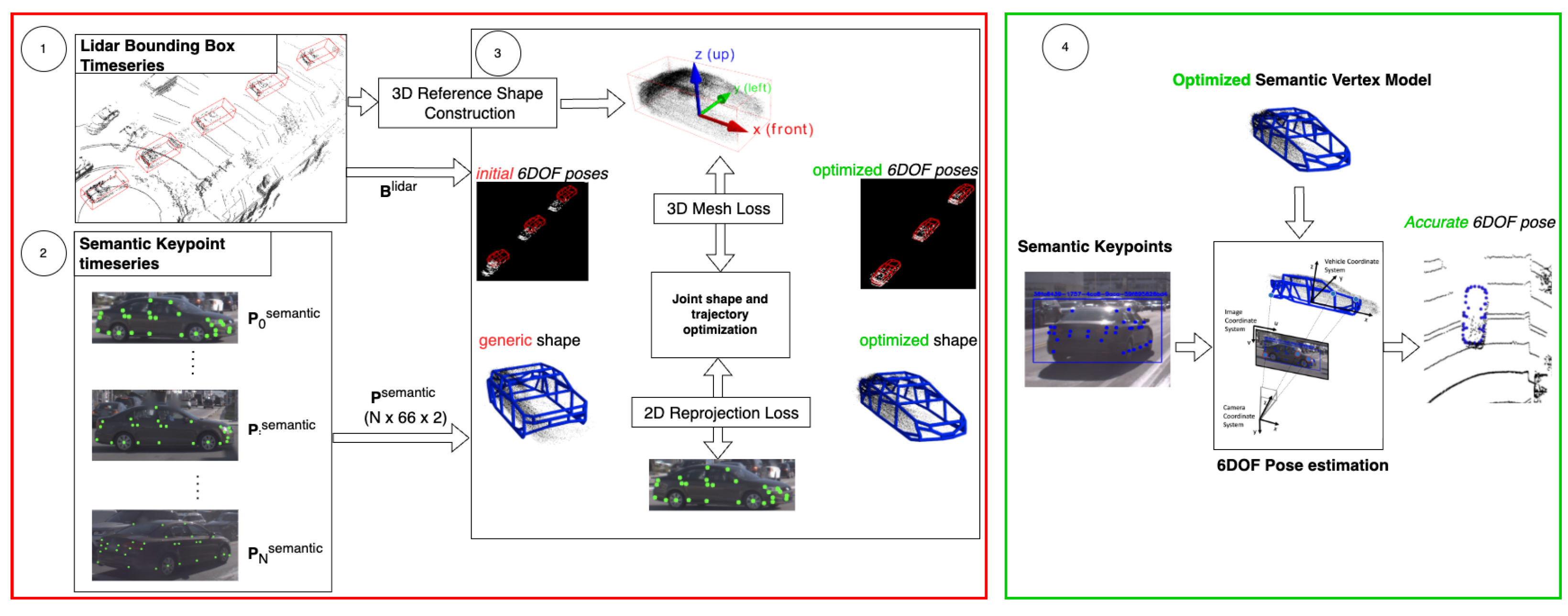
3. Materials and Methods

The goal of the algorithm is to reconstruct the semantic shape of a vehicle to enable subsequent camera-only localization. In this section, we describe our method in mathematical terms. The algorithm’s overview can be seen in Figure 2. The algorithm performs the following essential steps:

• The object reference shape is constructed using the LiDAR bounding box timeseries.
• The semantic keypoints are extracted, tracked and matched to the LiDAR bounding boxes throughout the trajectory.
• The shape and trajectory of the Semantic Mesh Model are optimized, minimizing 2D re-projection loss between the keypoints and vertices as well as 3D shape loss between the Semantic Mesh Model and the reference shape.
• The reconstructed Semantic Mesh Model can be used for single, or multi-image-based pose estimation.

Figure 2. This figure demonstrates the full process. The initial Reconstruction Phase is followed by an image-based 6DOF pose estimation. First, the target vehicle is tracked both in the LiDAR point-cloud timeseries and the image for semantic keypoint extraction. Next, the LiDAR reference shape is constructed, and the keypoint timeseries is filtered for faulty detections. Finally, the Semantic Mesh Model shape is optimized from the undeformed Semantic Mesh Model by minimizing 3D loss and the re-projection loss. This model is reusable for highly accurate single- and multi-view pose estimation.

Figure 2. This figure demonstrates the full process. The initial Reconstruction Phase is followed by an image-based 6DOF pose estimation. First, the target vehicle is tracked both in the LiDAR point-cloud timeseries and the image for semantic keypoint extraction. Next, the LiDAR reference shape is constructed, and the keypoint timeseries is filtered for faulty detections. Finally, the Semantic Mesh Model shape is optimized from the undeformed Semantic Mesh Model by minimizing 3D loss and the re-projection loss. This model is reusable for highly accurate single- and multi-view pose estimation.

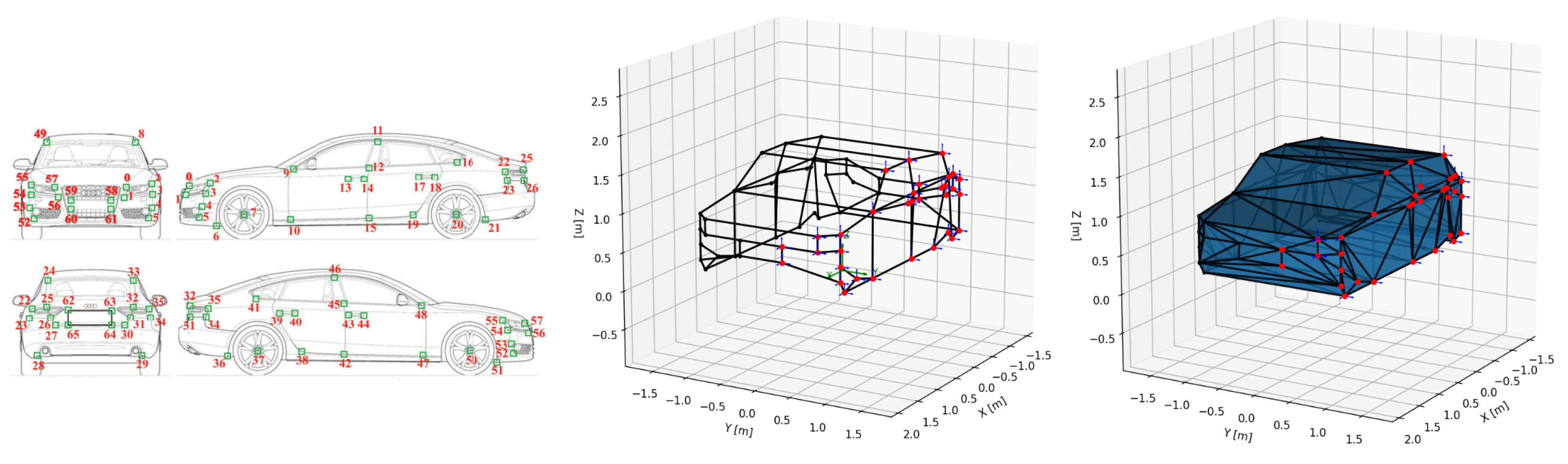
3.1. Problem Statement

Firstly, we define the world coordinate system as a single coordinate system to which all of the sensors are calibrated. In the tests on the Argoverse dataset, this is the dataset’s own world coordinate system; in our own experiments, this is the UTM coordinate system. We also define for each camera the camera coordinate system, which follows the OpenCV [41] convention. Next, the Semantic Mesh Model is defined as follows: we define the vehicle coordinate system following ISO 8855. The origin is at the center of the bottom face of the 3D bounding box of the vehicle. The X axis points forward along the vehicle’s longitudinal axis, the Y axis points left, laterally to the vehicle, and the Z axis points vertically up.

The deformable and symmetric Semantic Vertex Model, ${\mathbf{M}}^{semantic}$ is defined in our first work [15] as a structured set of 66 vertices representing semantically meaningful keypoints, which are associated with a distinct semantic label as defined in the ApolloCar3D dataset [14]. We add a brief introduction here for clarity. Formally,

$${\mathbf{M}}^{semantic}=[{\mathbf{m}}_1,{\mathbf{m}}_2,\dots ,{\mathbf{m}}_{66}],{\mathbf{m}}_j=[x,y,z]$$

(1)

where ${\mathbf{m}}_j$ are the 3D semantic vertices and ${\mathbf{M}}_{semantic}\in {\mathbb{R}}^{66\times 3}$. The vertices are arranged in such a way that for $j=1,2,\dots ,33$$m_j$ constitutes the left side of the vehicle. These vertices will be deformed during the optimization as follows:

$${\mathbf{m}}_j^{def}={\mathbf{m}}_j+{\mathbf{d}}_j,$$

(2)

where $d_j$ is the deformation vector for the j-th index, and $\mathbf{D}\in {\mathbb{R}}^{33\times 3}$ is the set of deformation vectors used. For $j=34,35,\dots ,66$$m_j$ is the right side, which due to the assumption of symmetry can be parametrized as follows:

$${\mathbf{m}}_j={\mathbf{T}}_{xz}{\mathbf{m}}_{(j-33)},$$

(3)

where

$${\mathbf{T}}_{XZ}=\left[\begin{array}{ccc}1& 0& 0\\ 0& -1& 0\\ 0& 0& 1\end{array}\right].$$

(4)

From here on, we refer to this deformation process as the deformation function

$${\mathbf{M}}^{deformed}=f^{deformation}({\mathbf{M}}^{semantic},D).$$

(5)

In this work, we extend this vertex model to a mesh model by defining faces between the vertices that create a watertight mesh from the semantic keypoints.

$${\mathcal{S}}^{\mathrm{semantic}}=({\mathbf{M}}^{\mathrm{semantic}},\mathcal{F}),$$

(6)

where the following apply:

• ${\mathbf{M}}^{\mathrm{semantic}}$ is the aforementioned vertex set.
• $\mathcal{F}={\left\{{\mathbf{f}}_k\right\}}_{k=1}^{N_f}$ is the set of triangular faces defined by vertex indices, creating a watertight manifold mesh representing the vehicle’s surface:

  $${\mathbf{f}}_k=[i,j,l],\mathrm{with}i,j,l\in \{1,\dots ,66\},k\in \{1,\dots ,N_f\}.$$

  (7)

The triangular faces were selected in such a way that they form a watertight mesh. The connectivity of the keypoints was defined manually so that the individual faces belong to semantically meaningful parts of the vehicle. For example, the headlight has four corners in the Semantic Vertex Model, so in order to define triangular faces, the plane of the headlight was divided into two faces (see Figure 3). All in all, we define 128 mesh faces, for exact face definitions refer to Appendix A.

The deformation of the mesh by deformation parameters $\mathbf{D}$ is defined by its vertex deformations, which are mathematically shown below:

$${\mathbf{S}}^{deformed}=(f^{deformation}({\mathbf{M}}^{semantic},\mathbf{D}),\mathcal{F})$$

(8)

The visualization of the undeformed Semantic Mesh Model can be observed in Figure 3.

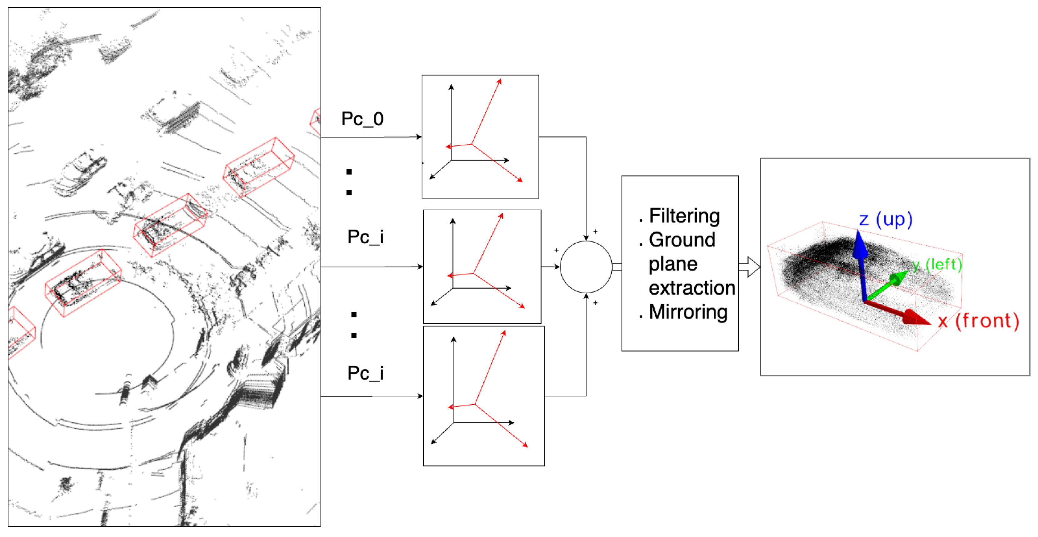
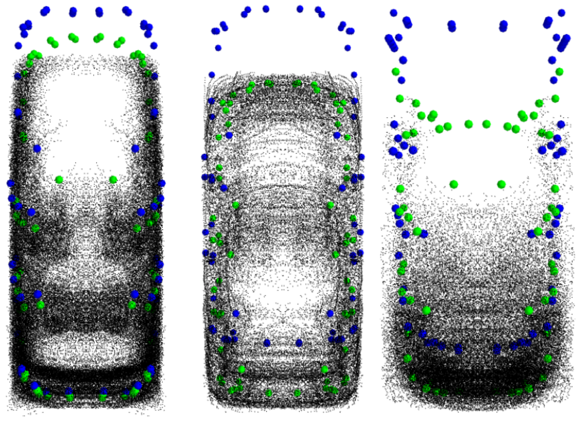
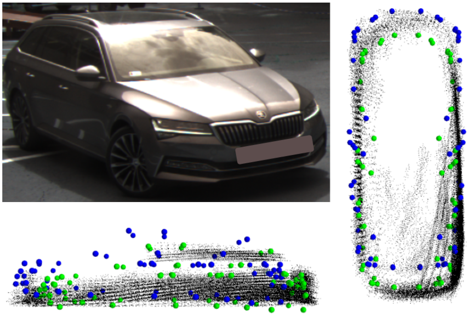
3.2. LiDAR-Based Reference Shape Reconstruction

In order to incorporate LiDAR data into the optimization, we construct a LiDAR Reference Point Cloud from a timeseries of LiDAR detections. Let a timeseries of LiDAR-based object detections be mathematically defined as a sequence of bounding boxes defined in the world coordinate system:

$$B_t=\{p_t,{\mathbf{R}}_t,S_t\},$$

(9)

where $p_t=(x_t,y_t,z_t)$ is the bottom center point position, ${\mathbf{R}}_t\in SO\left(3\right)$ is the orientation, and $S_t=(w_t,l_t,h_t)$ represents the dimensions (width, length, height) of the detected object at time t, this was transformed to the ego camera’s coordinate system as defined in the pinhole camera model [27].

We segment the complete point cloud in timeframe t${\mathcal{P}}_t$, keeping only points within the bounding box $B_t$. These points are named $p_{b,t}\in {\mathcal{P}}_t^B$, and are stored as. The segmented points are then translated and rotated into the target vehicle’s local coordinate system for each point at each time step:

$${\widehat{p}}_{b,t}^B={\mathbf{R}}_t^{\top }{\left(p_{b,t}-p_t\right)}^T$$

(10)

We concatenate these points into one set and name it the LiDAR Reference Point-cloud, mathematically, $P_B^{ref}$. This results in LiDAR measurements corresponding to an object, which was viewed as if the target was stationary, and the LiDAR was moved around it for the purpose of reconstructing its surface. However, in the setting of an AD dataset like Argoverse, this is often incomplete and noisy, containing points from various objects and the ground in addition to the target. We therefore use Ransac [42] to estimate the ground plane in the bottom 10% of points in the bounding box. We use outlier rejection and mirror the points onto the XZ plane of the bounding box, leveraging the fact that most road cars are symmetrical. This yields the final LiDAR Reference Point Cloud we can use to enforce the scale and shape the Semantic Mesh Model. The final output can be seen in Figure 4.

3.3. Keypoint Extraction and Fault Detection

Provided that there are cameras (one or more) that are calibrated and synchronized to the LiDAR point cloud, we record images $I_t$ corresponding to the point clouds at each timeframe t. We run a semantic keypoint detector, such as OpenPifPaf [33] or Yolov8-Pose [34], which were trained on the Apollocar3D dataset [14]. For each image, this yields a set of ${\mathbf{P}}_{t,c}^{semantic}\in {\mathbb{R}}^{66\times 3}$ keypoint detections for each c-th of the F cars in the image at time step t. There are 66 semantic keypoints within a detection, each defined as pixel coordinates, and an associated confidence value as $s_j={[u,v,confidence]}_j$. On the corresponding LiDAR frame, we detect l cars using a 3D object detector.

In order to find which car’s keypoint detection corresponds to the LiDAR detection, we use the camera’s calibration information and the pose of the vehicles as detected by the LiDAR. We take the deformable Semantic Mesh Model and move it to the target’s pose as detected by the LiDAR sensor. This is achieved as follows. For every vertex ${\mathbf{m}}_{\mathbf{i}}$ of the Semantic Mesh Model $\mathbf{M}{,}^{\int \rceil \Updownarrow ⊣\backslash \bigsqcup ⟩\rfloor }$, we apply the transform

$${\mathbf{m}}_{\mathbf{i}}^{\mathbf{\prime }}={\mathbf{m}}_{\mathbf{i}}{\mathbf{R}}_{\mathbf{t}}^{\mathbf{T}}+p_t,$$

(11)

yielding the transformed model ${\mathbf{M}}_{\mathbf{l}}^{\mathbf{\prime }\int \rceil \Updownarrow ⊣\backslash \bigsqcup ⟩\rfloor }$ for the l-th car. Then, we project the vertices into the image:

$${\mathbf{m}}_{\mathbf{i}}^{\mathbf{″}}=\mathbf{K}{\mathbf{m}}_{\mathbf{i}}^{\prime \mathbf{T}},$$

(12)

yielding the projected model ${\mathbf{M}}_{\mathbf{l}}^{\mathbf{″}\int \rceil \Updownarrow ⊣\backslash \bigsqcup ⟩\rfloor }$.

We select the keypoint detection for the given 3D bounding box by defining an error metric $Q_e$ between the projected Semantic Vertex Model and the detected semantic keypoints. $Q_e$ is defined as follows: First, the keypoints are normalized to the object detection size:

$${\mathbf{k}}_{\mathrm{norm}}^{\det }={\displaystyle \frac{{\mathbf{k}}_c^{\det }-\mathrm{mean}\left({\mathbf{k}}_c^{\det }\right)}{\mathrm{diag}\left({\mathbf{k}}_l^{\mathrm{proj}}\right)}},{\mathbf{k}}_{\mathrm{norm}}^{\mathrm{proj}}={\displaystyle \frac{{\mathbf{k}}_l^{\mathrm{proj}}-\mathrm{mean}\left({\mathbf{k}}_l^{\mathrm{proj}}\right)}{\mathrm{diag}\left({\mathbf{k}}_l^{\mathrm{proj}}\right)}}$$

(13)

Then, the keypoint error is determined:

$$e_{\mathrm{kp}}(c,l,t)={\displaystyle \frac{1}{N}}\sum _{j=1}^N{\parallel {\mathbf{k}}_{\mathrm{norm},j}^{\det }-{\mathbf{k}}_{\mathrm{norm},j}^{\mathrm{proj}}\parallel }_2$$

(14)

We also use an instance segmentation model Yolov8-mask [34] to detect the semantic mask of the targets. We compute the convex hull of the projected Semantic Vertex Model and find their IoU:

$$e_{\mathrm{hull}}(c,l,t)=max(0,{\tau }_{\mathrm{hull}}-\mathrm{IoU}(\mathrm{Hull}\left({\mathbf{k}}_l^{\mathrm{proj}}\right),{\mathcal{C}}_{t,c}))\times f_{\mathrm{penalty}}$$

(15)

Finally, the complete metric is found:

$$Q_e=e_{\mathrm{kp}}(c,l,t)+e_{\mathrm{hull}}(c,l,t)$$

(16)

and from the set of ${\mathbf{P}}_{t,i}^{semantic}$ detections, we calculate the following metric for each ${\mathbf{P}}_{t,i}^{semantic}$ in the set. We keep only the timeframes $t_{confirmed}$ where the semantic keypoints are available and correct.

3.4. Semantic Mesh Shape Optimization

Our objective is to recover both the deformation parameters $\mathbf{D}$ of the semantic mesh and the time-varying 6DOF pose $(\mathbf{Q},\mathbf{T}$ that jointly minimize (i) the 2D re-projection error of keypoints in every calibrated camera and (ii) the discrepancy between the deformed mesh and the LiDAR reference point cloud. The optimization parameters are defined as shown below:

$$\begin{array}{cc}\hfill & \mathbf{Q}=[{\mathbf{q}}_1,{\mathbf{q}}_2,\dots ,{\mathbf{q}}_N]\hfill \end{array}$$

(17)

$$\begin{array}{cc}\hfill & \mathbf{T}=[{\mathbf{t}}_1,{\mathbf{t}}_2,\dots ,{\mathbf{t}}_N]\hspace{1em}\hfill \end{array}$$

(18)

$$\begin{array}{cc}\hfill & \mathbf{D}=[{\mathbf{d}}_1,{\mathbf{d}}_2,\dots ,{\mathbf{d}}_{33}],\hfill \end{array}$$

(19)

where $\mathbf{Q}$ is a matrix of rotation quaternions, $\mathbf{T}$ is a matrix of translation vectors in the system’s coordinate frame, and $\mathbf{D}$ is the matrix of deformation parameters.

2D Keypoint Re-Projection Loss

Let ${\mathbf{K}}^{\left(c\right)}$ be the intrinsic matrix, ${\mathbf{R}}^{\left(c\right)}$ and ${\mathbf{t}}^{\left(c\right)}$ be the extrinsic parameters of camera c. For each frame t, camera c, and deformed 3D semantic vertex ${{\mathbf{m}}^{\prime }}_i$, the loss functions are formulated as follows:

$$L_{2\mathrm{D}}=\sum _{i=1}^N\sum _c\sum _{j\in J_i}{\parallel {\mathbf{s}}_{ijc}-{\mathbf{p}}_{ijc}\parallel }^2$$

(20)

subject to:

$${\mathbf{s}}_{ijc}={\mathbf{K}}^{\left(c\right)}\left[\begin{array}{c}{\mathbf{R}}^{\left(c\right)}\left[\begin{array}{c}{\mathbf{q}}_i{\mathbf{m}}_j^{def}{\mathbf{q}}_i^{-1}+{\mathbf{t}}_i\end{array}\right]{\mathbf{t}}^{\left(c\right)}\end{array}\right]$$

(21)

3D LiDAR Shape Loss

The Semantic Mesh Model is also aligned to the LiDAR reference shape, $P_B^{ref}=\{p_0,\dots p_n\}$ by also minimizing a 3D shape loss. This helps enforce the scale of the model and reduce unreasonable warping of the shape in cases of noisy 2D keypoint detections. The function combines point-to-plane, point-to-edge and Laplacian smoothing losses, all of which are readily implemented in the Pytorch3D library. Mathematically, the LiDAR shape loss is shown below:

$$L_{\mathrm{LiDAR}}={\lambda }_{\mathrm{f}}{L}_{\mathrm{face}}+{\lambda }_{\mathrm{e}}{L}_{\mathrm{edge}}+{\lambda }_{\mathrm{l}}{L}_{\mathrm{laplace}},$$

(22)

with $({\lambda }_{\mathrm{f}},{\lambda }_{\mathrm{e}},{\lambda }_{\mathrm{l}})=(10,1,1)$ in all experiments.

The point-to-plane loss measures how far reference LiDAR point ${\mathbf{p}}_n$ lies from the closest mesh face $f_k$ along the face normal, where $\mathcal{F}={\left\{f_k\right\}}_{k=1}^{N_f}$ are the faces of the Semantic Vertex Model. The pull of this loss is therefore in the normal direction of the mesh faces, helping the shape expand or contract to accurately capture the scale of the target. Additionally, since our Semantic Mesh Model has far fewer vertices compared to Autoshape [39], a point-to-point loss would pull the sparse vertices toward dense clusters in the inhomogeneous LiDAR reference shape. For face $f_k$ with unit normal ${\mathbf{n}}_k$ and a point on the face ${\mathbf{p}}_k^f$, the squared distance is

$$d^2\left({\mathbf{p}}_n,f_k\right)={\left({\mathbf{n}}_k^{\top }({\mathbf{p}}_n-{\mathbf{p}}_k^f)\right)}^2.$$

(23)

Averaging over all N points and choosing for each point the minimal squared distance to any of the $N_f$ faces yields the total face loss

$$L_{\mathrm{face}}={\displaystyle \frac{1}{N}}\sum _{n=1}^N\underset{k=1,\dots ,N_f}{min}{d}^2\left({\mathbf{p}}_n,f_k\right),$$

(24)

where each face $f_k$ has a unit normal ${\mathbf{n}}_k$ and centroid ${\mathbf{p}}_k^f$.

The point-to-edge loss acts in a similar fashion while also enforcing that the faces cannot expand perpendicularly to their normal direction. Thus, for the edges $\mathcal{E}={\left\{e_{\ell }\right\}}_{\ell =1}^{N_e}$, we calculate

$$L_{\mathrm{edge}}={\displaystyle \frac{1}{N}}\sum _{n=1}^N\underset{\ell =1,\dots ,N_e}{min}{∥{\mathbf{p}}_n-{\mathsf{\Pi }}_{e_{\ell }}\left({\mathbf{p}}_n\right)∥}_2^2.$$

(25)

where ${\mathsf{\Pi }}_{e_{\ell }}\left(\mathbf{p}\right)$ denotes the orthogonal projection of point ${\mathbf{p}}_n$ onto edge $e_{\ell }$.

In order to enforce smoothness of the resulting mesh, we calculate the Laplacian loss. Let $\mathbf{L}$ be the cotangent Laplacian of the undeformed mesh.

$$L_{\mathrm{lap}}={∥\mathbf{L}\left({\mathbf{M}}_0+\delta \right)∥}_F^2.$$

(26)

The Point to Plane, Point to Edge, and Laplacian loss functions are already part of the Pytorch3D library; please refer to its source code for more details at [43]. The novelty lies in the formulation of the Semantic Mesh Model and the Reference Lidar Shape between which the loss functions perform a comparison.

Thus, the total objective is the combination of the re-projection and LiDAR losses.

$$L(\Theta )=L_{2\mathrm{D}}+L_{\mathrm{LiDAR}}.$$

(27)

We minimize (27) using the PyTorch (version 2.0.1 with CUDA 11.7) implementation of the Adam optimizer. The above LiDAR loss functions are already part of the Pytorch3D library (corresponding to Pytorch and CUDA versions). The learning rate is controlled by a scheduler that reduces the learning rate by a factor of $0.5$ if the loss value does not decrease for 10 consecutive iterations. All deformation parameters $d_i$ are initialized to zero, while the camera poses $({\mathbf{R}}_t,{\mathbf{t}}_t)$ are seeded using the LiDAR-based estimates. The optimization runs for a maximum of 1000 iterations with early stopping triggered if the learning rate drops below $l_r={10}^{-6}$. The loss weights ${\lambda }_{\mathrm{f}},{\lambda }_{\mathrm{e}},{\lambda }_{\mathrm{l}}$ used in Equation (22) are fixed throughout the optimization for all scenarios.

3.5. N–View Pose Estimation

At runtime, leveraging the reconstructed Semantic Vertex Model, we estimate a rigid 6DOF pose for every tracked vehicle at each time step t, fusing information from all available synchronized cameras ${\left\{I_t^{\left(c\right)}\right\}}_{c=1}^C$. For every image $I_t^{\left(c\right)}$, detect the semantic keypoints with a pretrained detector [33]. We identify the target vehicle in order to pair the reconstructed model to the detection. This can be achieved by OCR-based license plate recognition or vehicle make and model recognition.

Given a reliable keypoint set for vehicle v, we solve a multi-view PnP problem in the least-squares sense:

$$\underset{{\mathbf{R}}_t,{\mathbf{t}}_t}{min}\sum _{c=1}^C\sum _{i=1}^{N_v}{w}_{t,i}^{\left(c\right)}{∥{\mathbf{k}}_{t,i}^{\left(c\right)}-{\mathbf{u}}_{t,i}^{\left(c\right)}({\mathbf{R}}_t,{\mathbf{t}}_t)∥}_2^2\mathrm{s}.\mathrm{t}.{\mathbf{R}}_t\in SO\left(3\right).$$

(28)

We initialize with the previous pose in the trajectory. Optionally, we employ the re-projection metric in Equation (16) to identify if the pose was incorrect.

4. Results

Our main contribution is the integration of the LiDAR measurements into the originally camera-only pipeline in [15]. In this section, we show that this enables a much higher level of fidelity of the Semantic Mesh Model, and once a vehicle is reconstructed, it can be localized more accurately from any viewpoint using only 2D keypoints compared to both the camera-only baseline [15] and the state-of-the-art BAAM [13].

We evaluate our method using the absolute pose error rather than traditional 3D object detection scores like 3D mean average precision (mAP). This measures the absolute 6DOF alignment error between the localized model and the ground truth providing a precise assessment in localization accuracy. 3D mAP, on the other hand, aggregates detection quality over all objects, obscuring the importance of fine-grained pose estimation in comparison to object presence detection.

Overall, our approach excels when the reconstruction of a vehicle can be guaranteed, and subsequently, its keypoints are detected accurately in the image. It focuses on minimizing the pose estimation error, whereas 3D object detection methods such as BAAM [13] focus on robustness to object presence detection. The question of which is more important is highly application-specific.

By reporting translational and rotational errors of the compared methods in meters and degrees, we demonstrate a targeted metric directly reflecting the improvements in 6DOF pose estimation achieved by our LiDAR-enhanced pipeline.

4.1. Evaluation Methodology

We evaluate our contributions through four main experiments. First, we assess the effectiveness of our reconstruction pipeline using a single-LiDAR, single-camera setup on the Argoverse dataset [16], comparing it directly against Semantic [15] and BAAM [13]. Second, we measure the classification accuracy of our proposed pose quality metric. Third, we analyze the robustness–accuracy tradeoff between our method (MM-VSM) and BAAM, which was selected due to its state-of-the-art neural-based 6DOF pose estimation. Finally, we conduct ablation studies to isolate and quantify the impact of LiDAR loss versus multi-view reconstruction.

For consistency with prior evaluations [15], we primarily utilize the Argoverse dataset, as it provides annotated images, LiDAR data, and tracking labels. We also conduct further ablations using data collected from the ZalaZONE proving ground to specifically evaluate the impact of LiDAR loss in the presence of multi-view data.

As our method is not a simple object detector—it can only estimate poses of vehicles it has reconstructed first—the evaluation metrics and methodology are non-trivial. We only wish to evaluate whether the accuracy of the pose estimation as object detection (meaning object presence detection) depends largely on our input 2D semantic keypoints and whetherr or not the model was reconstructed previously. In our experiments, therefore, we evaluate on the subset of the datasets that was detected by OpenPifPaf and BAAM, and we compare which estimates the detected object’s pose most accurately. BAAM was chosen as the primary baseline due to its superior performance compared to other classical geometry-based approaches (see [15]) or deep learning-based approaches [14,37,44]. These either rely on geometrical assumptions which are not always true or are outperformed by BAAM, or their source is not available.

In summary, direct comparisons with our previous method, Semantic [15], and BAAM [13] clearly illustrate our improvements and the advantages and disadvantages of our method.

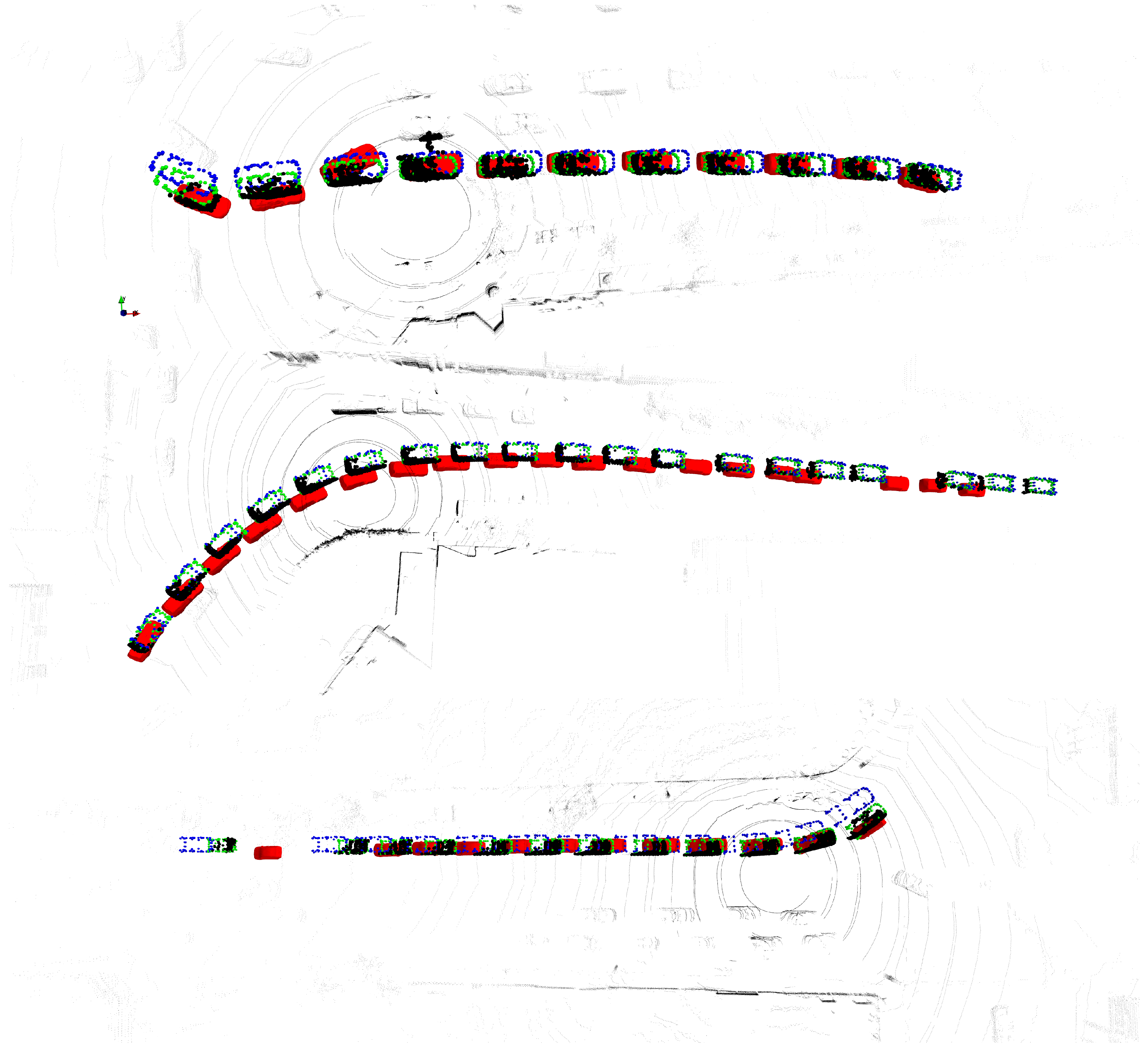
4.2. Improved Performance on the Argoverse Dataset

We qualitatively and quantitatively evaluate the effect of the integration of our LiDAR-enhanced semantic mesh reconstruction on the publicly available Argoverse dataset [16].

In our experiments, we use the absolute pose error (APE), which is the difference between the target 6DOF pose and the labeled GT 6DOF pose. We differentiate between translational APE or $e_t^{\mathrm{trans}}$ and rotational APE or $e_t^{\mathrm{rot}}$, which are mathematically defined as follows, starting with the ground truth ${\mathbf{T}}_t^{\mathrm{gt}}$ and estimated ${\mathbf{T}}_t^{\mathrm{est}}$ 6DOF poses:

$${\mathbf{T}}_t^{\mathrm{gt}}=\left(\begin{array}{cc}{\mathbf{R}}_t^{\mathrm{gt}}& {\mathbf{t}}_t^{\mathrm{gt}}\\ {\mathbf{0}}^{\top }& 1\end{array}\right)\in \mathrm{SE}\left(3\right),{\mathbf{T}}_t^{\mathrm{est}}=\left(\begin{array}{cc}{\mathbf{R}}_t^{\mathrm{est}}& {\mathbf{t}}_t^{\mathrm{est}}\\ {\mathbf{0}}^{\top }& 1\end{array}\right)$$

(29)

The difference (error) of the two, named $\Delta {\mathbf{T}}_t$, is shown below:

$$\Delta {\mathbf{T}}_t={\left({\mathbf{T}}_t^{\mathrm{gt}}\right)}^{-1}{\mathbf{T}}_t^{\mathrm{est}}=\left(\begin{array}{cc}{\mathbf{R}}_{\Delta ,t}& {\mathbf{t}}_{\Delta ,t}\\ {\mathbf{0}}^{\top }& 1\end{array}\right),$$

(30)

where

$${\mathbf{R}}_{\Delta ,t}={\left({\mathbf{R}}_t^{\mathrm{gt}}\right)}^{\top }{\mathbf{R}}_t^{\mathrm{est}},{\mathbf{t}}_{\Delta ,t}={\mathbf{t}}_t^{\mathrm{est}}-{\mathbf{t}}_t^{\mathrm{gt}}.$$

(31)

Thus, the rotational and translational APE is

$$e_t^{\mathrm{trans}}={\parallel {\mathbf{t}}_{\Delta ,t}\parallel }_2,e_t^{\mathrm{rot}}=arccos\left(\frac{\mathrm{trace}\left(R_{\Delta ,t}\right)-1}{2}\right)\in [0,\pi ].$$

(32)

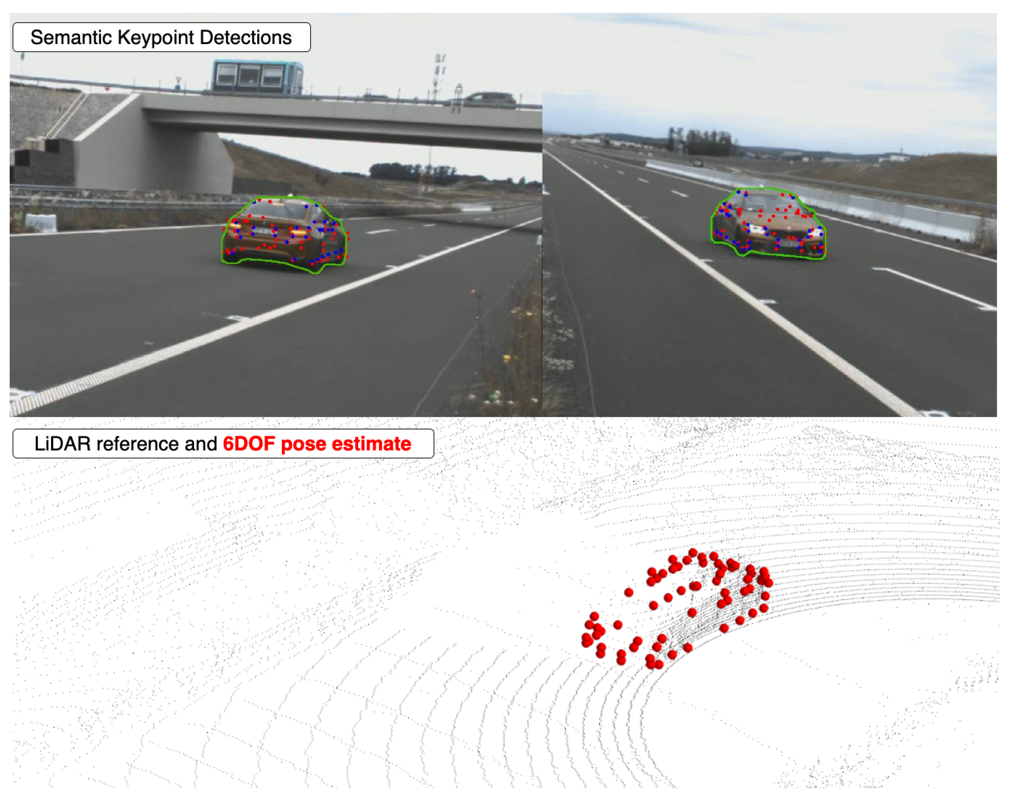
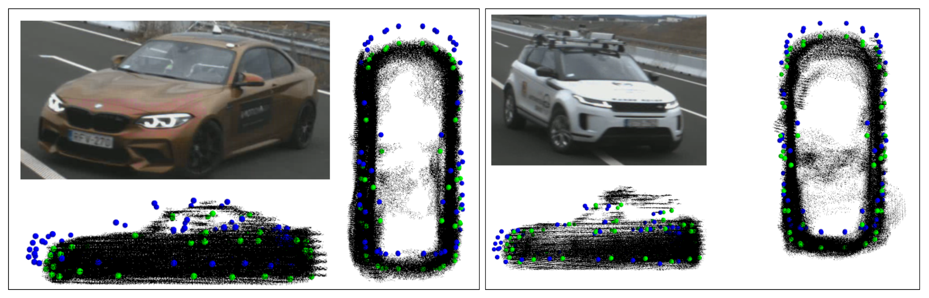
4.2.1. Qualitative Evaluation

To complement our quantitative gains (see below), we present specific, qualitative improvements. Firstly, the LiDAR-enhanced novel method produces a Semantic Mesh Model which fits the LiDAR point cloud more tightly. This means that the reconstructed shape more accurately captures the 3D locations of the semantic vertices on the target vehicle. This in turn will lead to a more accurate camera-based pose estimation. To show the qualitative improvements, we selected three test trajectories on the Argoverse dataset.

Figure 5 shows the shape reconstruction improvements. It can be observed that although the camera-based method captures the shape closely, there can be a slight scale error in the reconstruction, which is eliminated by the LiDAR-assisted pipeline. The corresponding improvement in the pose estimation can be observed in Figure 6. Note how the novel method improves the scale correctness significantly.

There are cases where the reconstruction fails completely in the camera-only reconstruction in [15]. This usually is the result of faulty initial pose estimates and erroneous keypoint detections misleading the optimization. Figure 7 shows a prime example of this. Through the use of the novel method, the error is corrected.

The more accurate scale leads to significantly improved single image-based pose estimation. This qualitatively is visible in Figure 6, which contains the result of the single-image-based pose estimates using the reconstructed models from Figure 5. Figure 6 contains reference LiDAR point clouds, the original camera-only method’s results and the outputs of BAAM [13] for visual comparison.

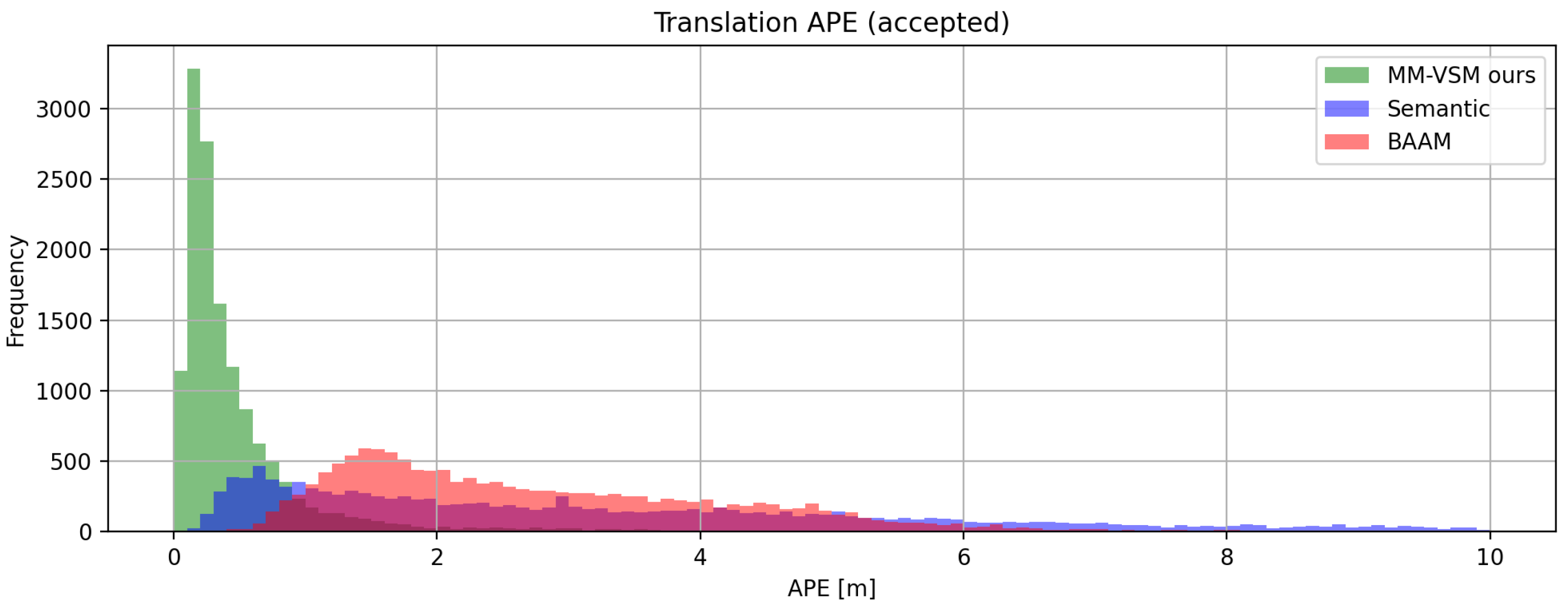
4.2.2. Quantitative Evaluation

Quantitatively, we show that our method shows significant improvements in APE over Semantic and BAAM on the successfully reconstructed trajectories. It is important to note that both Semantic and MM-VSM require a reconstruction step in order to be able to estimate poses. This means that we can only evaluate pose estimates on trajectories that are sufficiently long and detected by OpenPifPaf consistently enough to be reconstructed. However, as our goal is not to evaluate an object detector but to improve the accuracy of pose estimation of already detected objects, our statistical analysis stands. Please note that for general, in-vehicle autonomous driving, 3D object detection applications metrics that describe object presence detection accuracy (such as mAP) may be better. Please also note that BAAM or OpenPifPaf were not retrained to the Argoverse dataset in order to show general applicability of as-is pretrained models.

In the histogram, the following can be observed:

• MM-VSM produces the most accurate pose estimates.
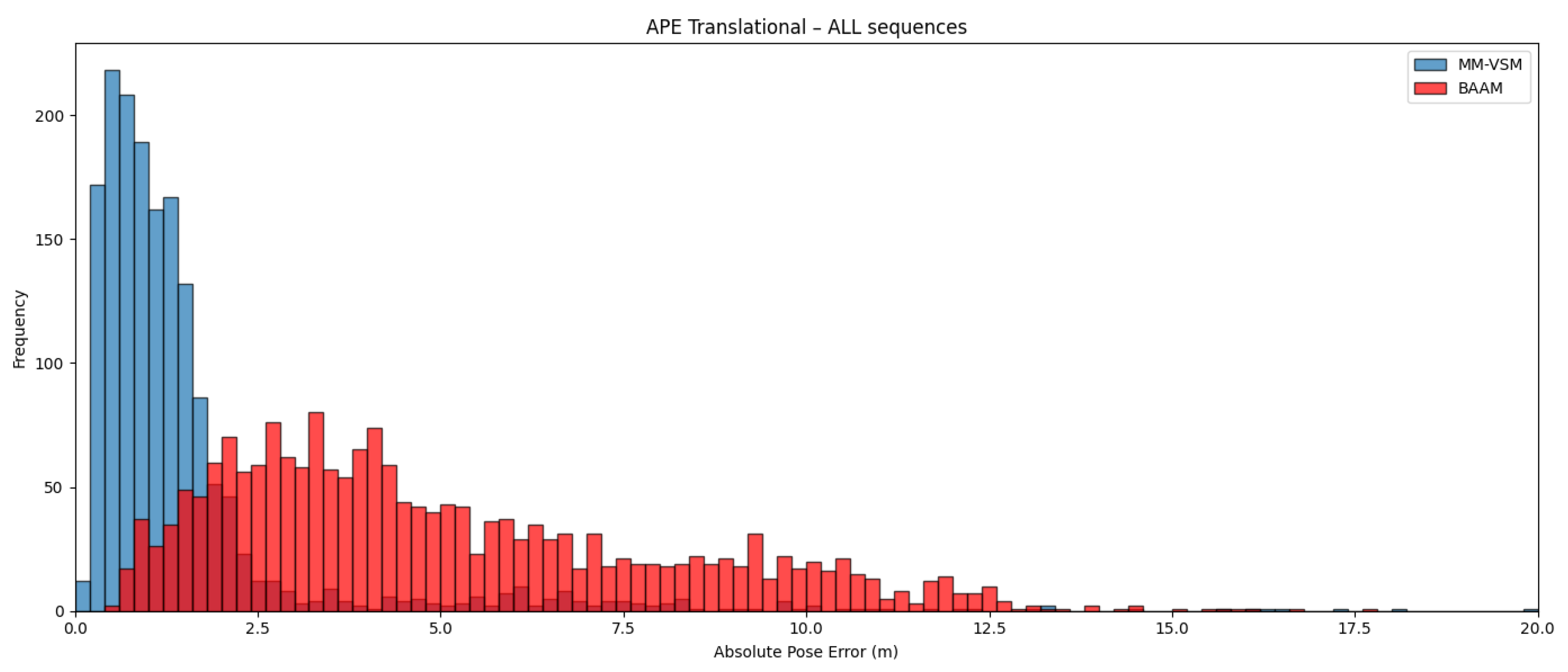
• Semantic produces the second-best peak accuracy with a large tail indicating many failed cases.
• BAAM produces larger but more consistent errors in APE than Semantic.

These findings support our assumptions that using LiDAR data to produce a geometrically correct Semantic Mesh Model reduces erroneous reconstructions, therefore significantly improving the pose estimation robustness of Semantic on the Argoverse dataset.

In addition to the histogram (Figure 8), we also present a numerical analysis. Because our pose estimation relies on a direct least squares problem, there are cases where the result diverges. This means that simply calculating averages is misleading, as a handful of extremely large errors can severely degrade the results. We therefore classify extremely large errors as failures and perform a failure analysis. We use two separate gates: a standard and a strict gate.

Table 1. Frames discarded by each acceptance gate ($N_{\mathrm{tot}}=15,407$). Bold numbers indicate the lowest failure rate per gate.

	Default Gate (10 m, 45°)		Strict Gate (5 m, 30°)
Method	Removed	Failure [%]	Removed	Failure [%]
MM-VSM (ours)	1319	8.56	1781	11.56
Semantic [15]	2436	15.81	5527	35.87
BAAM [13]	834	5.41	2 204	14.31

reports how many frames each method loses when the standard gate (10 m, 45°) is applied and when the gate is tightened to 5 m, 30°. MM-VSM (ours) ranks second-best for default robustness but becomes the most reliable once the stricter threshold is used. Semantic [15] is the most fragile under both settings.

On the frames that are not classified as failures, we perform a deeper statistical evaluation.

Table 2. Absolute pose error on accepted frames (mean $\mu$, standard deviation $\sigma$, median, 95-percentile $P_{95}$). Boldface marks the best (lowest mean).

	Translation [m]			Rotation [°]
Method	$\mathbf{\mu }\mathbf{\pm }\mathbf{\sigma }$	Median	${\mathbf{P}}_{\mathbf{95}}$	$\mathbf{\mu }\mathbf{\pm }\mathbf{\sigma }$	Median	${\mathbf{P}}_{\mathbf{95}}$
MM-VSM (ours)	0.56$\mathbf{\pm }$0.94	0.29	1.79	6.35$\mathbf{\pm }$6.49	4.47	20.61
Semantic [15]	3.18$\pm$2.39	2.59	8.16	7.82$\pm$7.20	5.47	23.48
BAAM [13]	2.79$\pm$1.50	2.44	5.51	10.99$\pm$4.09	9.95	18.30

and

Table 3. Local-frame roll, pitch, and yaw error on accepted frames (mean $\mu \pm \sigma$ in degrees). Lower is better; best mean per axis in bold.

Axis [°]	MM-VSM (Ours)	Semantic [15]	BAAM [13]
Roll	2.60$\pm$3.23	2.78$\pm$3.26	2.88$\pm$1.87
Pitch	3.28$\pm$4.86	3.62$\pm$3.67	9.71$\pm$3.41
Yaw	3.09$\pm$4.66	4.78$\pm$6.73	2.97$\pm$3.43

present the error statistics on the frames that survive the default gate. In addition to the mean ($\mu$) and standard deviation ($\sigma$), we list the median and the 95-percentile ($P_{95}$) to characterize distribution tails. The results clearly show that on the non-failed detections, our method produces superior pose estimation compared to the relevant methods. This is true only if the reconstructed models for the vehicles are available and the object is detected in the image by OpenPifPaf.

4.2.3. Findings

Based on both histogram-based and numerical analysis, we make the following findings:

• Translational accuracy. MM-VSM significantly improves the robustness and accuracy of Semantic, producing the best translational APE on the evaluated frames, and also failing fewer times than BAAM.
• Rotational accuracy. In total rotational APE, MM-VSM outperforms BAAM and significantly improves Semantic.
• Local-frame RPY alignment. Using roll/pitch/yaw defined in the target’s own axes, MM-VSM is best on roll (2.60°) and pitch (3.28°), whereas BAAM is best on yaw (2.97°). Semantic sits consistently in the middle. Thus, BAAM’s overall rotation error stems primarily from roll–pitch misalignment, which is indicative of the training bias, due to the shifted camera position and viewpoint.
• Accuracy vs. robustness. MM-VSM delivers the best accuracy and passes the strict gate most often (lowest failure $11.56\%$). BAAM is the most robust under the default gate ($5.41\%$ failures) but trades off accuracy; Semantic is weakest on both gates.
• Histograms. Looking at the head of the histograms, Semantic offers better peak accuracy compared to BAAM, and MM-VSM produces large improvements over both. This indicates that our LiDAR pipeline succesfully removes failures correcting Semantic’s errors.
• Axis-specific trends. MM-VSM excels at stabilizing vehicle roll and pitch; BAAM delivers the sharpest yaw on average, which benefits heading-aware downstream tasks.

In summary, MM-VSM occupies the sweet spot on the accuracy–robustness spectrum, while BAAM favours robustness at the expense of roll–pitch accuracy. Note that BAAM (and its OpenPifpaf feature extractor) were trained on ApolloCar3D, whose slightly different camera viewpoint induces a static bias on the Argoverse validation suite—visible in BAAM’s roll–pitch, and slight pose errors.

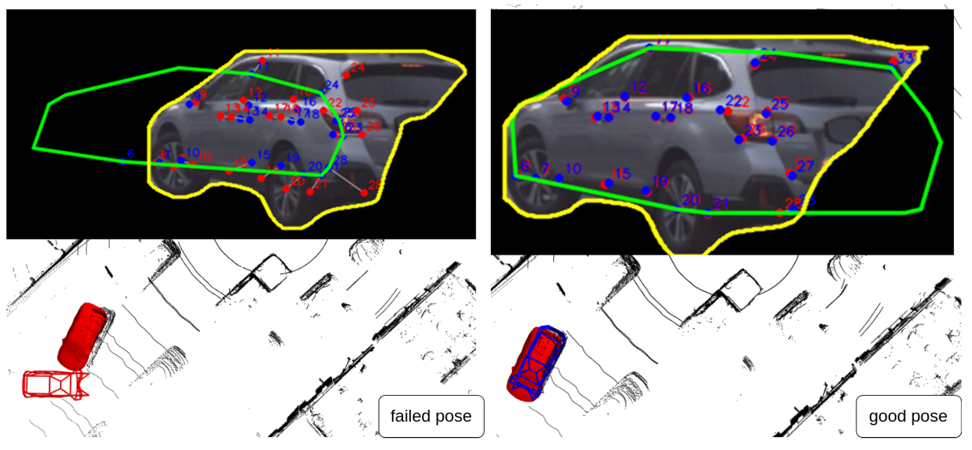
4.3. Failure Analysis and Failure Detecion

There are cases where our pose estimation fails regardless of how accurate the reconstructed model is. In this section, we firstly examine why this happens, and secondly, we evaluate our pose quality metric on the failure’s detection.

4.3.1. Failure Analysis-Occlusion

One of the method’s biggest weaknesses compared to a deep learning method like BAAM [13] is its occlusion resistance. Firstly, if the keypoints are not visible in the image timeseries, their corresponding Semantic Vertices cannot be reconstructed (unless their symmetrical pair is detected). Secondly, our pose estimation is the solution to a multi-view pose estimation problem from 2D–3D keypoint correspondences. This has well-studied properties [14,27,30], showing its performance is best when the most possible keypoints are visible and they do not lie on the same plane. In the single-view case, at least four non-coplanar points need to be detected, and in the multi-view case, at least three corresponding points (or their mirrored point in the Semantic Mesh Model) must be detected for the pose estimation to be theoretically solvable [27].

Qualitatively, we show a failed pose estimation under partial occlusion in Figure 9. This is a typical case where the detected Semantic Keypoints are almost coplanar, resulting in a strong local minimum that the algorithm becomes stuck in. On the right, as soon as point 33 is also detected, the points are no longer near coplanar; therefore, the algorithm finds the global optimum.

Unfortunately, the Argoverse 1 dataset does not currently contain actual “occlusion” data even though it’s present in the API, its set to 0 everywhere. Therefore, we cannot quantitatively verify this, although future work will include research on occlusion-resistant pose estimation.

Although the quantitative evaluation of occlusion resistance is not possible here, similar research in the literature [14] indicates that the likelihood of failure for occluded single-view cases is quite high for our algorithm. BAAM handles occlusion especially well; that is a large part of its contribution.

However, we would also like to point out that in a Smart Parking garage application, the reduction in implementation costs versus LiDAR-based alternatives or 3D annotation costs for each sensor may be so high that an arbitrary number of cameras may be installed. This enables the construction of such a system where occlusion is scarce.

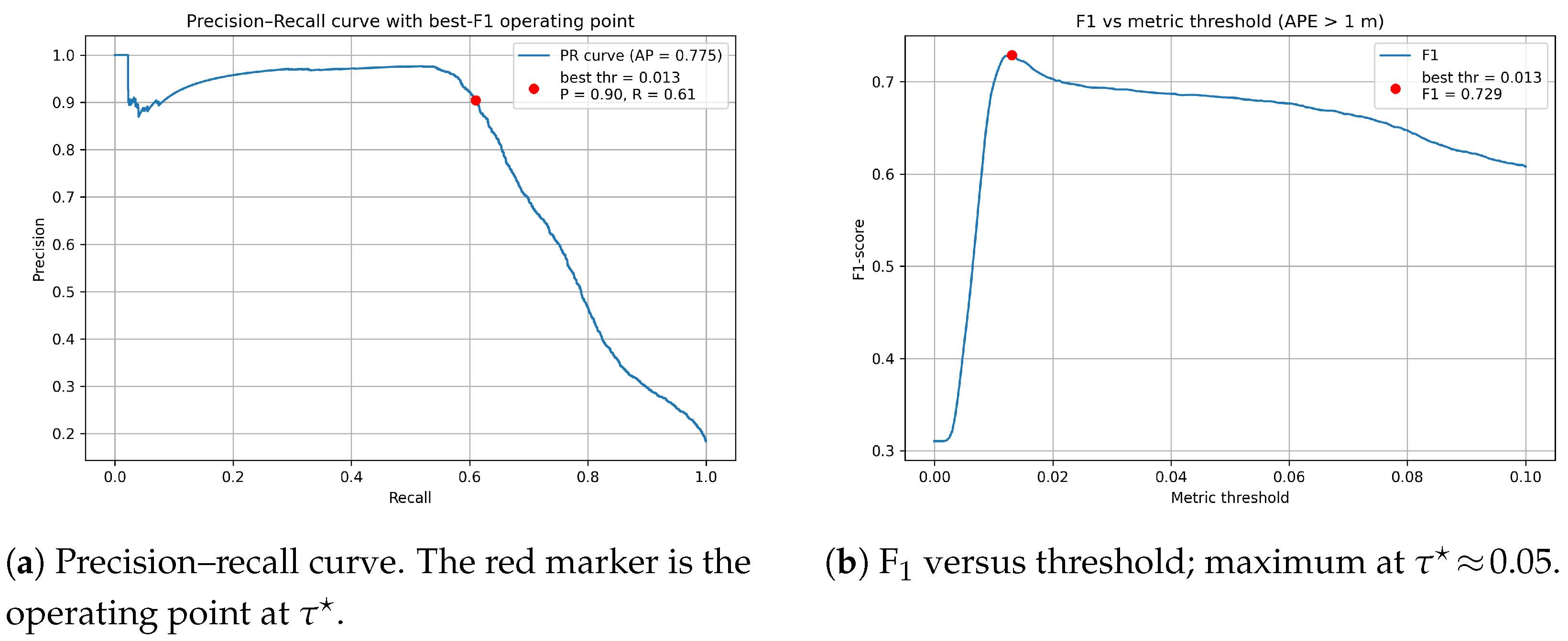
4.3.2. Pose Quality Metric

In failure cases, it may be useful to be able to recognize the fault. We previously defined a pose quality metric (apart from the obvious re-projection error). In order to use this, the object must be also semantically segmented in the image. We evaluate how accurate this metric is and what the ideal classification threshold is. This is accomplished using the following statistical method: let ${\mathbf{Q}}_{\mathbf{pose}}$ denote the pose quality metric. Higher values indicate poorer alignment. We classify a frame as a failure if its translation absolute pose error (APE) exceeds $1\mathrm{m}$:

$$y=\left\{\begin{array}{cc}1,\hfill & \mathrm{if}{\mathrm{APE}}_{\mathrm{trans}}>1\mathrm{m},\hfill \\ 0,\hfill & \mathrm{otherwise},\hfill \end{array}\right.\widehat{y}\left(\tau \right)=\left\{\begin{array}{cc}1,\hfill & \mathrm{if}{\mathbf{Q}}_{\mathrm{pose}}>\tau ,\hfill \\ 0,\hfill & \mathrm{otherwise}.\hfill \end{array}\right.$$

(33)

The overall discrimination performance is summarized by the precision–recall curve (Figure 10a). The average precision (AP), computed as

$$\mathrm{AP}={\int }_0^{1}P\left(R\right)dR=0.78,$$

(34)

indicates good performance. Sorting frames by decreasing ${\mathbf{Q}}_{\mathrm{pose}}$ correctly identifies failures nearly 80% of the time, making it an effective ranking metric.

To select a single practical threshold, we maximized the $F_1$ score over thresholds in the range where ${\mathbf{Q}}_{\mathrm{pose}}$ varies significantly (0 to 0.1):

$$F_1\left(\tau \right)={\displaystyle \frac{2P\left(\tau \right)R\left(\tau \right)}{P\left(\tau \right)+R\left(\tau \right)}}.$$

(35)

Figure 10b shows an optimal threshold around

$${\tau }^{★}\approx 0.05,P\left({\tau }^{★}\right)=0.64,R\left({\tau }^{★}\right)=0.23,F_1\left({\tau }^{★}\right)=0.32.$$

(36)

The practical implications of these results are that very low scores (${\mathbf{Q}}_{\mathrm{pose}}<0.01$) strongly indicate reliability. In a tracking application, ${\tau }^{★}=0.05$ is a reliable acceptance threshold. Overall, the metric provides a reliable high-precision safety filter. Low values strongly confirm accurate pose estimation, while values above the identified threshold reliably indicate the need for caution or a fallback strategy.

Figure 9 shows our quality metric in action. In rare cases, when the target vehicle is partially occluded, the pose estimation fails even though the keypoint detections are accurate. This, however, is detected by our pose quality metric. Note that it is specifically in these cases that BAAM [13] outperforms our method, which can also be observed in the Figure 10.

In conclusion of the experimental evaluation, it can be observed that the LiDAR-based pipeline significantly improves reconstruction accuracy and robustness, producing fewer errors and failures. This additionally means that the pose estimations are also more accurate. Our method, therefore, extends the state of the art in image-based vehicle pose estimation. We also show that our pose quality metric is capable of identifying faulty pose estimates, increasing the practical usability of the algorithm.

5. Ablation Study on ZalaZONE

In this section, we extend Semantic [15] to multi-view and multi-modal reconstruction from a monocular-only reconstruction. In this experiment, we evaluate the effect of multi-view alone versus multi-view and multi-modal reconstruction.

In this experiment, we use our 3D LiDAR-based detector presented first in [45]. We use our novel pipeline to reconstruct the vehicle’s Semantic Mesh Model. We compare camera-only multi-view and camera–LiDAR reconstruction methods for shape accuracy. Then, we conduct multi-view pose estimation on the image sequences and evaluate the performance of both LiDAR-camera and multi-view reconstructions.

Qualitatively, the improvements of the LiDAR integration mainly center around scale correctness. Although the camera-based reconstruction provides an accurate 3D shape, the LiDAR improves this further. Additionally, the deformations and the pose is ambiguous in the camera-only reconstruction; therefore, the semantic vertices are slightly incorrectly shifted in the vehicle’s local coordinate system. The LiDAR measurements enforce the correctness, as seen below, in Figure 11.

Quantitatively, we make modifications to the evaluation compared to [15]. We calculate the translational APE of the centroid of the LiDAR 3D bounding boxes compared to the centroid as opposed to the origin of the reconstructed Semantic Vertex Model. This is because our LiDAR detector also produces errors, and it is not fair to assume that its bottom center will match the local origin of the Semantic Vertex Model as a ground truth metric. Figure 12 shows the effect on pose estimation of using LiDAR over a synchronous multi-view reconstruction. The improvements are slight but consistent in our experiments.

6. Real-World Application

In this section, we present the first real-world application of our algorithm. Provided that a LiDAR-equipped reconstruction area is available, our method can be used for highly accurate 6DOF pose estimation based on a single calibrated CCTV camera. We demonstrate this in the form of a smart parking garage application, where it can be guaranteed that the vehicles are reconstructed when entering the complex, thus enabling single or multi-view pose estimation in the rest of the system. This would significantly reduce costs compared to LiDAR-based systems in such scenarios. The concept is explained in detail in Figure 13.

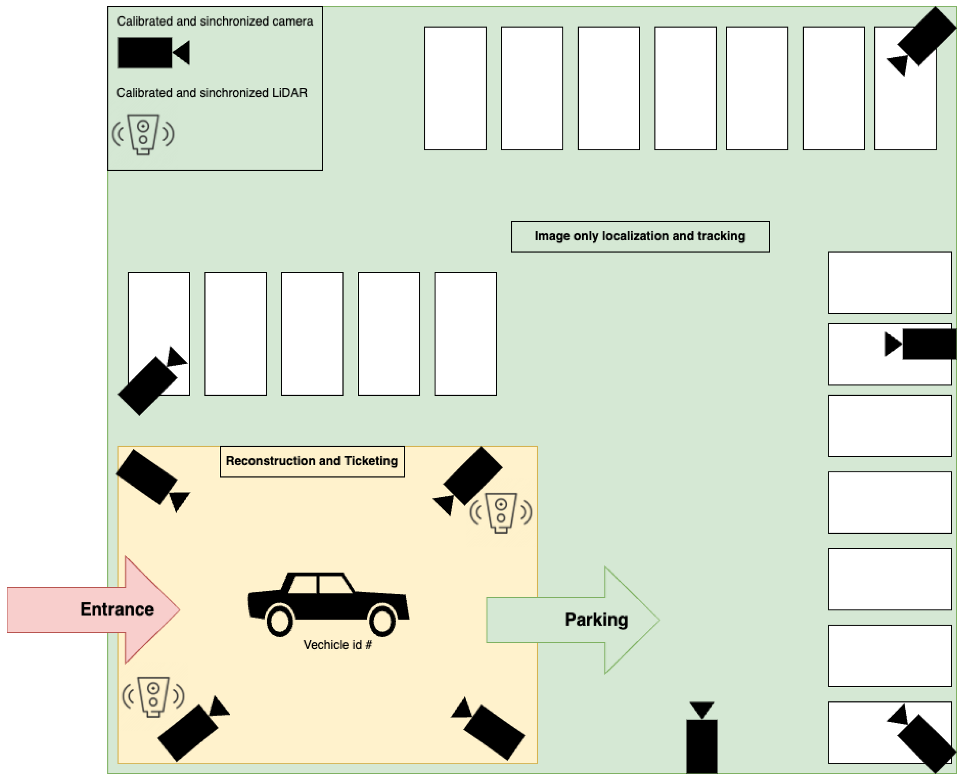
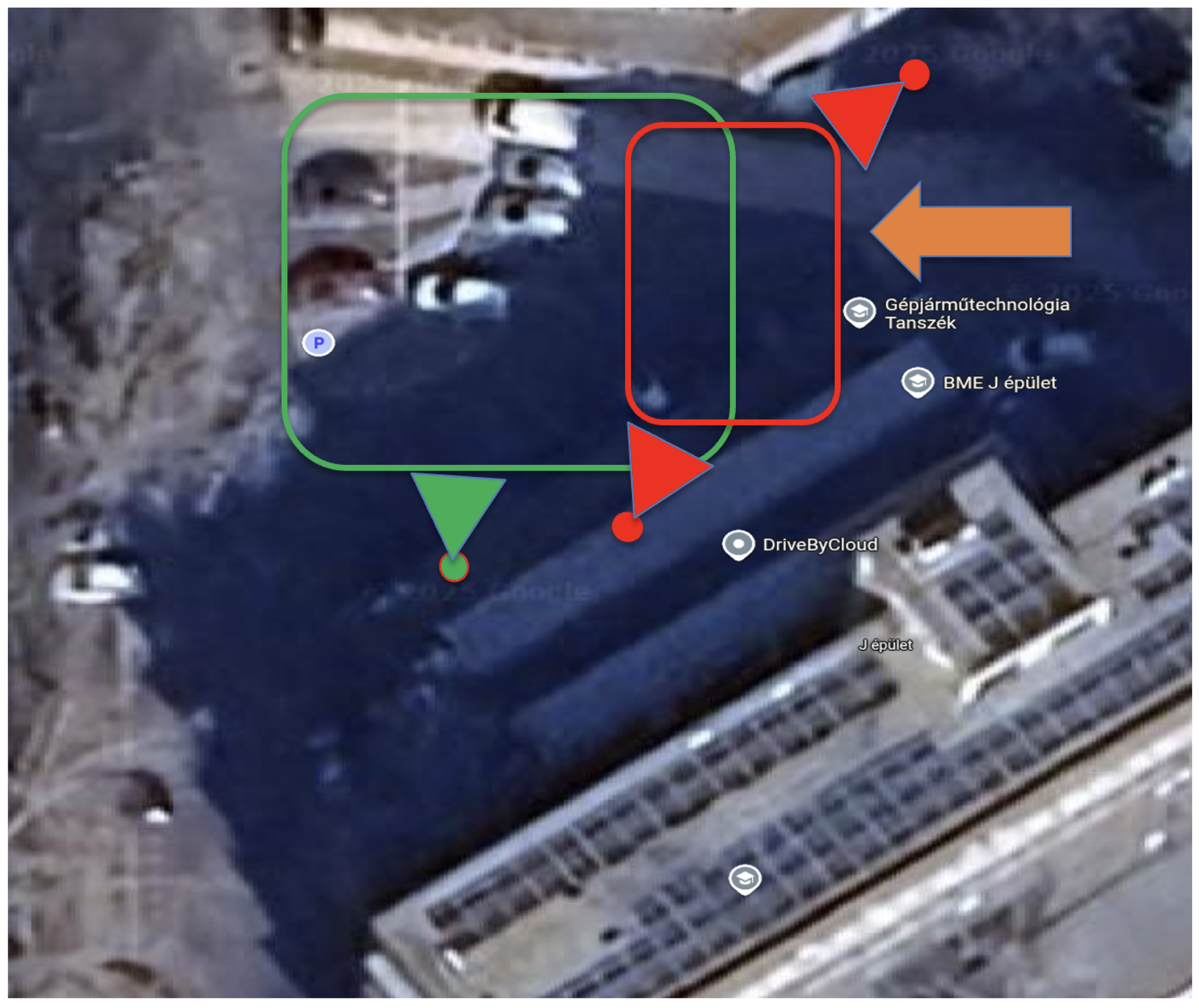
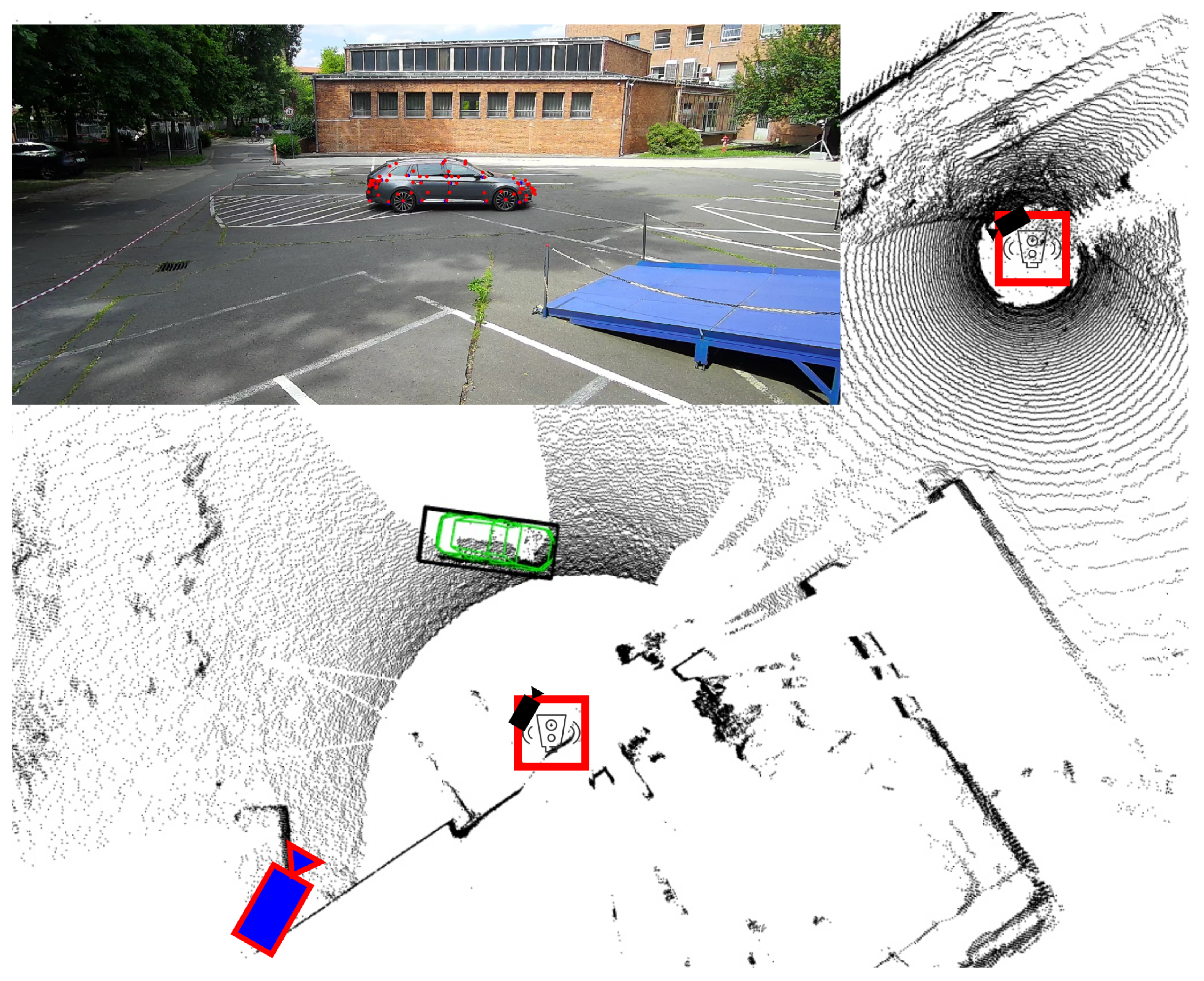
6.1. BME Parking Area

We demonstrate the above concept in a real-world experiment at a BME (Budapest University of Technology and Economics) parking area. We set up two LiDAR–camera sensor Ouster (San Francisco, CA, USA) and FLIR (Richmond, BC, Canada) stations and define a reconstruction area, which is shown in red in the satellite image (Figure 14). This is where the Semantic Mesh Model is created corresponding to a vehicle. We drive a variety of vehicles through this area. Then, we use a cheap Dahua IP camera (Hangzhou, China) to accurately localize the vehicle. Please note that this single-frame localization yields training-free 6DOF pose estimates; therefore, the planarity of the ground or other environmental constraints do not play a role. This cannot be reproduced by other algorithms to the best of our knowledge.

6.2. Experimental Setup

We use Flir Pointgrey measurement cameras (Richmond, BC, Canada) and Ouster LiDARs (San Francisco, CA, USA) for the reconstruction areas. We use a Dahua IP camera for the localization. The sensor resolutions are 1616 × 1240 × 3 RGB for the Flir cameras running at 10 fps and QHD for the IP camera. The LiDARs were also run at 10 fps.

We intrinsically calibrate the cameras using Zhang’s method as implemented in OpenCV. We calibrate every sensor extrinsically to the UTM coordinate system using a highly accurate GPS sensor. We measure the UTM coordinates of specific cracks and markings on the road, and we select corresponding pixels and points manually from the point cloud and the images. We use a simple PnP solver (OpenCV) to calibrate the cameras extrinsically and an RMSE minimization to calibrate the LiDARs initially; then, we refine this estimate using ICP. Both take place in CloudCompare.

The algorithm is run on a high-performance gaming PC with an Intel processor (14900K) and Nvidia GPU (RTX4090) (Santa Clara, CA, US). Ubuntu and RTMaps are used for sensor synchronization. As the vehicles are driving slowly, the fact that the RTSP stream from the IP camera has a slight delay and the Flir cameras are not hardware synchronized does not influence the results. For a LiDAR-based detector, we use the classical detector in [45].

Evaluation

We use five cars for the experiment. They each conduct an initial drive through the reconstruction area, where their Semantic Mesh Model is constructed with the LiDAR-assisted pipeline. The reconstruction process takes 10–30 s depending on the length of the trajectory. Thereafter, they conduct several parking maneuvers, during which the pose estimation is calculated solely based on the IP camera. We compare the detected poses from BAAM and MM-VSM to the LiDAR detector. The results of the experiment are consistent with earlier results (see Figure 15), showing scale and shift improvements over the camera-only method. Concerning the pose estimation, BAAM’s error increases significantly, as this is a very different camera and very different viewpoint from its training set. This underlines our method’s advantage and the fact that BAAM would need retraining before use on a setup like this.

Below, in Figure 16, we show an example image of the pose estimation. The green pose estimate is made using the IP camera only. It fits the reference point cloud perfectly.

Quantitatively, the errors are calculated similarly to the ZalaZONE measurements. On this dataset, our LiDAR detector [45] actually performs worse than the presented method, as there is no LiDAR coverage from every angle in the pose estimation area. In a reproduced experiment, we recommend to construct a path for reconstruction in which the LiDAR cloud covers every angle of the vehicles in order to use bounding box fitting detectors for the reference shape construction. Therefore, the following histogram is only a comparison of the LiDAR detector and the IP camera-based pose estimation as opposed to a ground-truth evaluation of our method. The result, however, is that the top of the histogram is around 0.5 m, which means that both detector’s errors could be similar. See Figure 17. Numerically, the results are found in

Table 4. Absolute pose translation error on accepted frames (mean $\mu$ ± $\sigma$, median, P95). Lower is better; best mean in bold.

Method	$\mathit{\mu }\pm \mathit{\sigma }$	Median	P95
MM-VSM (ours)	1.40$\pm$1.48	1.02	4.85
BAAM [13]	4.42$\pm$2.37	3.97	9.13

.

This section showed that the presented algorithm is usable in the real-world smart parking area application without the need for expensive retraining.

7. Discussion and Future Research

In this section, we discuss the results presented above.

7.1. Advantages and Runtime Performance

Firstly, it is shown that our method is less dependent on context and pretraining than BAAM. This means that for our method, no training data are needed: only successful reconstructions. Secondly, if the reconstruction can be guaranteed (such as in the parking garage application), our method offers very precise pose estimation in low occlusion cases.

At runtime, our method achieves far faster predictions compared to BAAM. The runtime performance did not change compared to Semantic [15]. OpenPifpaf can run on a RTX 4090 GPU with an Intel i9 core between 5 and 10 Hz on a size 2 batch of 808 × 680 images without exerting a load of over 20% on the GPU. BAAM, on the other hand, runs at less than 2 Hz. Our pose estimation pipeline uses Scipy, and its time for a single object is a few milliseconds, depending on the actual and previous poses. This makes our method real-time capable on two sensor stations and a powerful PC. If in the future a faster, more accurate keypoint detector is proposed, our method can integrate it much faster than BAAM.

7.2. Limitations

The most significant limitation of our algorithm is its reliance on the performance of the semantic keypoint detector. If no keypoints are detected, our method does not provide a pose estimate. This warrants further research on 2D semantic keypoint estimation techniques. Additionally, the re-identification of vehicles still poses a challenge, although make and model recognition could mitigate this. We plan on performing experiments to verify this; however, there are no currently available datasets containing sequence annotations, LiDAR point clouds and camera images, and most importantly vehicle-type annotations. This presents a research gap.

Our method struggles with cases of severe occlusion compared to deep learning methods such as BAAM [13]. In a parking garage environment, this can be mitigated by adequate camera coverage, meaning there will be no occlusion in the scene of a setup like the BME experiment. Nevertheless, this warrants further research, as no smart parking garage dataset has been proposed to date. Additionally, the implementation algorithms taking advantage of target motion and other contextual constraints such as road planarity (when available) presents a future research opportunity to handle these cases.

7.3. Future Research

With the expanding network of sensor-equipped smart roadside infrastructure, cooperative perception algorithms are evolving rapidly. However, on a highway section, which can consist of many hundreds of kilometers, the choice of sensors matters significantly. As the highway has controlled access routes, our algorithm enables the significant reduction of LiDAR sensors needed. In order to test this, we plan to evaluate the effectiveness of our method on the soon-to-be launched M1-M7 sensor system in Hungary, which is a smart-road section of the M1–M7 Motorway equipped with state-of-the-art sensors.

One of the most significant weaknesses of the proposed method is the reliance on the pretrained OpenPifPaf model, which was trained on the Apollocar3D dataset. This contains images only from a given perspective and context, meaning that the performance of the 2D detector is degraded slightly in different contexts and on vehicles not present in the training set. However, the accurate localization and re-projection of the Semantic Mesh Model vertices may enable the automatic 2D annotation of novel views. This concept will be explored in future research.

Currently, our method reconstructs the Semantic Mesh Model offline on a recorded sequence of data. Future research will include the possibility of online, on the fly reconstruction. Note that this does not inhibit its current applicability in the presented contexts.

8. Conclusions

This article presented a novel pipeline for enhancing Semantic Vertex Model reconstruction accuracy, building upon [15]. The algorithm improves the reconstruction of a vehicle’s model significantly by integrating LiDAR reference measurements into the shape optimization. The result is a Semantic Mesh Model consisting of faces, edges and semantically meaningful vertices, the latter of which can be detected in images by keypoint detectors such as OpenPifPaf. This 2D detection, combined with the known Semantic Mesh Model, may be used for accurate 6DOF pose estimation in various contexts without retraining.

The integration of the LiDAR pipeline into the reconstruction process clearly improves the accuracy of the resulting vehicle shapes and thereby the pose estimation as shown both quantitatively and qualitatively on the Argoverse dataset.

The presented method enables the implementation of a cooperative perception system for a smart parking garage while reducing dependency on LiDAR coverage significantly. We show in a real-world experiment that the reconstructed Semantic Mesh Model enables accurate 6DOF pose estimation using only a cheap IP camera, which is a feat that comparable methods simply cannot reproduce.

References

1. Ebrahimi Soorchaei, B.; Razzaghpour, M.; Valiente, R.; Raftari, A.; Fallah, Y.P. High-definition map representation techniques for automated vehicles. Electronics 2022, 11, 3374. [Google Scholar] [CrossRef]
2. Geiger, A.; Lenz, P.; Urtasun, R. Are we ready for autonomous driving? The kitti vision benchmark suite. In Proceedings of the 2012 IEEE Conference on Computer Vision and Pattern Recognition, Providence, RI, USA, 16–21 June 2012; pp. 3354–3361. [Google Scholar]
3. Zimmer, W.; Wardana, G.A.; Sritharan, S.; Zhou, X.; Song, R.; Knoll, A.C. Tumtraf v2x cooperative perception dataset. In Proceedings of the IEEE/CVF Conference on Computer Vision and Pattern Recognition, Seattle, WA, USA, 16–22 June 2024; pp. 22668–22677. [Google Scholar]
4. Xiang, H.; Zheng, Z.; Xia, X.; Xu, R.; Gao, L.; Zhou, Z.; Han, X.; Ji, X.; Li, M.; Meng, Z.; et al. V2x-real: A largs-scale dataset for vehicle-to-everything cooperative perception. In Proceedings of the European Conference on Computer Vision, Milan, Italy, 29 September–4 October 2024; Springer: Berlin/Heidelberg, Germany, 2024; pp. 455–470. [Google Scholar]
5. Yu, H.; Yang, W.; Ruan, H.; Yang, Z.; Tang, Y.; Gao, X.; Hao, X.; Shi, Y.; Pan, Y.; Sun, N.; et al. V2x-seq: A large-scale sequential dataset for vehicle-infrastructure cooperative perception and forecasting. In Proceedings of the IEEE/CVF Conference on Computer Vision and Pattern Recognition, Vancouver, BC, Canada, 17–24 June 2023; pp. 5486–5495. [Google Scholar]
6. Qu, D.; Chen, Q.; Bai, T.; Lu, H.; Fan, H.; Zhang, H.; Fu, S.; Yang, Q. SiCP: Simultaneous Individual and Cooperative Perception for 3D Object Detection in Connected and Automated Vehicles. In Proceedings of the 2024 IEEE/RSJ International Conference on Intelligent Robots and Systems (IROS), Abu Dhabi, United Arab Emirates, 14–18 October 2024; pp. 8905–8912. [Google Scholar]
7. Liu, J.; Wang, P.; Wu, X. A Vehicle–Infrastructure Cooperative Perception Network Based on Multi-Scale Dynamic Feature Fusion. Appl. Sci. 2025, 15, 3399. [Google Scholar] [CrossRef]
8. Nagy, R.; Török, Á.; Petho, Z. Evaluating V2X-Based Vehicle Control under Unreliable Network Conditions, Focusing on Safety Risk. Appl. Sci. 2024, 14, 5661. [Google Scholar] [CrossRef]
9. Chang, C.; Zhang, J.; Zhang, K.; Zhong, W.; Peng, X.; Li, S.; Li, L. BEV-V2X: Cooperative birds-eye-view fusion and grid occupancy prediction via V2X-based data sharing. IEEE Trans. Intell. Veh. 2023, 8, 4498–4514. [Google Scholar] [CrossRef]
10. Gao, Y.; Wang, P.; Li, X.; Sun, M.; Di, R.; Li, L.; Hong, W. MonoDFNet: Monocular 3D Object Detection with Depth Fusion and Adaptive Optimization. Sensors 2025, 25, 760. [Google Scholar] [CrossRef] [PubMed]
11. Yan, L.; Yan, P.; Xiong, S.; Xiang, X.; Tan, Y. Monocd: Monocular 3d object detection with complementary depths. In Proceedings of the IEEE/CVF Conference on Computer Vision and Pattern Recognition, Seattle, WA, USA, 16–22 June 2024; pp. 10248–10257. [Google Scholar]
12. Yang, L.; Zhang, X.; Yu, J.; Li, J.; Zhao, T.; Wang, L.; Huang, Y.; Zhang, C.; Wang, H.; Li, Y. MonoGAE: Roadside monocular 3D object detection with ground-aware embeddings. IEEE Trans. Intell. Transp. Syst. 2024, 25, 17587–17601. [Google Scholar] [CrossRef]
13. Lee, H.J.; Kim, H.; Choi, S.M.; Jeong, S.G.; Koh, Y.J. BAAM: Monocular 3D pose and shape reconstruction with bi-contextual attention module and attention-guided modeling. In Proceedings of the IEEE/CVF Conference on Computer Vision and Pattern Recognition, Vancouver, BC, Canada, 17-24 June 2023; pp. 9011–9020. [Google Scholar]
14. Song, X.; Wang, P.; Zhou, D.; Zhu, R.; Guan, C.; Dai, Y.; Su, H.; Li, H.; Yang, R. Apollocar3d: A large 3d car instance understanding benchmark for autonomous driving. In Proceedings of the IEEE/CVF Conference on Computer Vision and Pattern Recognition, Long Beach, CA, USA, 15–20 June 2019; pp. 5452–5462. [Google Scholar]
15. Cserni, M.; Rövid, A. Semantic Shape and Trajectory Reconstruction for Monocular Cooperative 3D Object Detection. IEEE Access 2024, 12, 167153–167167. [Google Scholar] [CrossRef]
16. Chang, M.F.; Lambert, J.; Sangkloy, P.; Singh, J.; Bak, S.; Hartnett, A.; Wang, D.; Carr, P.; Lucey, S.; Ramanan, D.; et al. Argoverse: 3d tracking and forecasting with rich maps. In Proceedings of the IEEE/CVF Conference on Computer Vision and Pattern Recognition, Long Beach, CA, USA, 15–20 June 2019; pp. 8748–8757. [Google Scholar]
17. Chen, R.; Gao, L.; Liu, Y.; Guan, Y.L.; Zhang, Y. Smart roads: Roadside perception, vehicle-road cooperation and business model. IEEE Network 2024, 39, 311–318. [Google Scholar] [CrossRef]
18. Yu, H.; Luo, Y.; Shu, M.; Huo, Y.; Yang, Z.; Shi, Y.; Guo, Z.; Li, H.; Hu, X.; Yuan, J.; et al. Dair-v2x: A large-scale dataset for vehicle-infrastructure cooperative 3d object detection. In Proceedings of the IEEE/CVF Conference on Computer Vision and Pattern Recognition, New Orleans, LA, USA, 18–24 June 2022; pp. 21361–21370. [Google Scholar]
19. Xu, R.; Xia, X.; Li, J.; Li, H.; Zhang, S.; Tu, Z.; Meng, Z.; Xiang, H.; Dong, X.; Song, R.; et al. V2v4real: A real-world large-scale dataset for vehicle-to-vehicle cooperative perception. In Proceedings of the IEEE/CVF Conference on Computer Vision and Pattern Recognition, Vancouver, BC, Canada, 17–24 June 2023; pp. 13712–13722. [Google Scholar]
20. Bai, Z.; Wu, G.; Barth, M.J.; Liu, Y.; Sisbot, E.A.; Oguchi, K. Pillargrid: Deep learning-based cooperative perception for 3d object detection from onboard-roadside lidar. In Proceedings of the 2022 IEEE 25th International Conference on Intelligent Transportation Systems (ITSC), Macau, China, 8–12 October 2022; pp. 1743–1749. [Google Scholar]
21. Qiao, D.; Zulkernine, F.; Anand, A. CoBEVFusion Cooperative Perception with LiDAR-Camera Bird’s Eye View Fusion. In Proceedings of the 2024 International Conference on Digital Image Computing: Techniques and Applications (DICTA), Perth, Australia, 27–29 November 2024; pp. 389–396. [Google Scholar]
22. Wei, S.; Wei, Y.; Hu, Y.; Lu, Y.; Zhong, Y.; Chen, S.; Zhang, Y. Asynchrony-robust collaborative perception via bird’s eye view flow. Adv. Neural Inf. Process. Syst. 2023, 36, 28462–28477. [Google Scholar]
23. Eskandar, G. An empirical study of the generalization ability of lidar 3d object detectors to unseen domains. In Proceedings of the IEEE/CVF Conference on Computer Vision and Pattern Recognition, Seattle, WA, USA, 16–22 June 2024; pp. 23815–23825. [Google Scholar]
24. Zhi, P.; Jiang, L.; Yang, X.; Wang, X.; Li, H.W.; Zhou, Q.; Li, K.C.; Ivanović, M. Cross-Domain Generalization for LiDAR-Based 3D Object Detection in Infrastructure and Vehicle Environments. Sensors 2025, 25, 767. [Google Scholar] [CrossRef]
25. Vincze, Z.; Rövid, A.; Tihanyi, V. Automatic label injection into local infrastructure LiDAR point cloud for training data set generation. IEEE Access 2022, 10, 91213–91226. [Google Scholar] [CrossRef]
26. Hu, Y.; Lu, Y.; Xu, R.; Xie, W.; Chen, S.; Wang, Y. Collaboration helps camera overtake lidar in 3d detection. In Proceedings of the IEEE/CVF Conference on Computer Vision and Pattern Recognition, Vancouver, BC, Canada, 17–24 June 2023; pp. 9243–9252. [Google Scholar]
27. Hartley, R.; Zisserman, A. Multiple View Geometry in Computer Vision; Cambridge University Press: Cambridge, UK, 2003. [Google Scholar]
28. Lowe, D.G. Distinctive Image Features from Scale-Invariant Keypoints. Int. J. Comput. Vis. 2004, 60, 91–110. [Google Scholar] [CrossRef]
29. Rublee, E.; Rabaud, V.; Konolige, K.; Bradski, G. ORB: An efficient alternative to SIFT or SURF. In Proceedings of the 2011 International Conference on Computer Vision, Barcelona, Spain, 6–13 November 2011; pp. 2564–2571. [Google Scholar]
30. Lepetit, V.; Moreno-Noguer, F.; Fua, P. EPnP: An accurate O(n) solution to the PnP problem. Int. J. Comput. Vis. 2009, 81, 155–166. [Google Scholar] [CrossRef]
31. Mur-Artal, R.; Montiel, J.M.M.; Tardos, J.D. ORB-SLAM: A versatile and accurate monocular SLAM system. IEEE Trans. Robot. 2015, 31, 1147–1163. [Google Scholar] [CrossRef]
32. Chen, C.; Jiang, X. Multi-View Metal Parts Pose Estimation Based on a Single Camera. Sensors 2024, 24, 3408. [Google Scholar] [CrossRef] [PubMed]
33. Kreiss, S.; Bertoni, L.; Alahi, A. Openpifpaf: Composite fields for semantic keypoint detection and spatio-temporal association. IEEE Trans. Intell. Transp. Syst. 2021, 23, 13498–13511. [Google Scholar] [CrossRef]
34. Jocher, G.; Chaurasia, A.; Qiu, J. Ultralytics YOLOv8 Software, Version 8.2.2; Ultralytics: London, UK, 2023. Available online: https://github.com/ultralytics/ultralytics (accessed on 14 June 2025).
35. Pavlakos, G.; Zhou, X.; Chan, A.; Derpanis, K.G.; Daniilidis, K. 6-dof object pose from semantic keypoints. In Proceedings of the 2017 IEEE International Conference on Robotics and Automation (ICRA), Singapore, 29 May–3 June 2017; pp. 2011–2018. [Google Scholar]
36. Barowski, T.; Szczot, M.; Houben, S. 6DoF vehicle pose estimation using segmentation-based part correspondences. In Proceedings of the 2019 IEEE Intelligent Transportation Systems Conference (ITSC), Auckland, New Zealand, 27–30 October 2019; pp. 573–580. [Google Scholar]
37. Ke, L.; Li, S.; Sun, Y.; Tai, Y.W.; Tang, C.K. Gsnet: Joint vehicle pose and shape reconstruction with geometrical and scene-aware supervision. In Proceedings of the Computer Vision–ECCV 2020: 16th European Conference, Glasgow, UK, 23–28 August 2020; Proceedings, Part XV 16. pp. 515–532. [Google Scholar]
38. He, T.; Soatto, S. Mono3d++: Monocular 3d vehicle detection with two-scale 3d hypotheses and task priors. In Proceedings of the AAAI Conference on Artificial Intelligence, Honolulu, HI, USA, 27 January–1 February 2019; Volume 33, pp. 8409–8416. [Google Scholar]
39. Liu, Z.; Zhou, D.; Lu, F.; Fang, J.; Zhang, L. Autoshape: Real-time shape-aware monocular 3d object detection. In Proceedings of the IEEE/CVF International Conference on Computer Vision, Montreal, QC, Canada, 10–17 October 2021; pp. 15641–15650. [Google Scholar]
40. Schörner, P.; Conzelmann, M.; Fleck, T.; Zofka, M.; Zöllner, J.M. Park my car! Automated valet parking with different vehicle automation levels by v2x connected smart infrastructure. In Proceedings of the 2021 IEEE International Intelligent Transportation Systems Conference (ITSC), Indianapolis, IN, USA, 19–22 September 2021; pp. 836–843. [Google Scholar]
41. Bradski, G.; Kaehler, A. OpenCV Library Software, Version 4.11; Intel Corporation: Santa Clara, CA, USA, 2000. Available online: https://opencv.org (accessed on 14 June 2025).
42. Fischler, M.A.; Bolles, R.C. Random sample consensus: A paradigm for model fitting with applications to image analysis and automated cartography. Commun. ACM 1981, 24, 381–395. [Google Scholar] [CrossRef]
43. PyTorch3D Developers. PyTorch3D: Loss Functions. 2025. Available online: https://pytorch3d.readthedocs.io/en/latest/modules/loss.html (accessed on 7 June 2025).
44. Chabot, F.; Chaouch, M.; Rabarisoa, J.; Teuliere, C.; Chateau, T. Deep manta: A coarse-to-fine many-task network for joint 2d and 3d vehicle analysis from monocular image. In Proceedings of the IEEE Conference on Computer Vision and Pattern Recognition, Honolulu, HI, USA, 21–26 July 2017; pp. 2040–2049. [Google Scholar]
45. Rovid, A.; Tihanyi, V.; Cserni, M.; Csontho, M.; Domina, A.; Remeli, V.; Vincze, Z.; Szanto, M.; Szalai, M.; Nagy, S.; et al. Digital twin and cloud based remote control of vehicles. In Proceedings of the 2024 IEEE International Conference on Mobility, Operations, Services and Technologies (MOST), Dallas, TX, USA, 1–3 May 2024; pp. 154–167. [Google Scholar]
Figure 1. This figure depicts a frame from our experiments on the ZalaZONE proving ground. The semantic keypoint estimates are visible (top) alongside the 6DOF pose estimate of the Semantic Mesh Model’s vertices as reconstructed by our novel approach and localized by the camera-only multi-view pose estimation.
Applsci 15 06930 g001
Figure 3. This figure depicts the semantic keypoint definitions from [14] (left), the original Semantic Vertex Model [15], and the new Semantic Mesh Model (right).
Applsci 15 06930 g003
Figure 4. The process of LiDAR reference shape extraction. A LiDAR detector tracks the object and segments its point cloud within the bounding box. These points are transformed to the target’s local coordinate system and merged. Next, filtering, ground removal and mirroring take place. On the right, the completed reference LiDAR model can be observed.
Applsci 15 06930 g004
Figure 5. This figure shows the improvements over [15] with regard to shape reconstruction. In blue, the semantic vertices reconstructed by [15], in green the current results, and in black the reference LiDAR shape.
Applsci 15 06930 g005
Figure 6. In this figure, the improvements of MM-VSM (green) over BAAM [13] (red) and Semantic [15] (blue) estimation can be observed on three demonstration trajectories from the Argoverse dataset. These are the qualitative pose estimates in the world coordinate system with the LiDAR points as backgrounds. Semantic and MM-VSM use their respective previously reconstructed Semantic Vertex Model and Semantic Mesh Model for single-image-based pose estimation.
Applsci 15 06930 g006
Figure 7. This is an example of a failed reconstruction produced by the image-only method [15] plotted in blue. The LiDAR-assisted correction is plotted in green.
Applsci 15 06930 g007
Figure 8. Translational APE histogram. In green the APE histogram of MM-VSM, in blue Semantic [15], and in red BAAM [13].
Applsci 15 06930 g008
Figure 9. This figure depicts the detection process of a pose failure. The top half illustrates our pose quality metric. The reprojected Semantic Mesh Model silhouette (yellow), keypoints (blue), and the detected instance segmentation mask by YOLO [34] (green) and semantic keypoints (red). The bottom half illustrates the associated pose estimates. On the left, the failed pose estimate (red wire-frame) as classified by our pose quality metric, and on the right, the (blue wire-frame), also correctly classified. The red mesh is the output of BAAM [13], which performs better under occlusion in this case.
Applsci 15 06930 g009
Figure 10. Behavior of the quality metric as an online detector of pose failures (APEtrans > 1m).
Applsci 15 06930 g010
Figure 11. This figure shows two examples of the slight scale and shift improvements of our method over the camera-only method. Blue and Green dots are the camera-only and camera-lidar reconstructions.
Applsci 15 06930 g011
Figure 12. This histogram shows the comparison of errors of the pose estimates made by our multi-view pose estimator. The green shows the error of using the LiDAR-assisted Semantic Mesh Models, and the blue shows the error of the camera-only multi-view reconstruction’s performance. The results show a slight but clear improvement.
Applsci 15 06930 g012
Figure 13. This diagram demonstrates the perception system that our algorithm enables. The strategically deployed reconstruction area is equipped by dense LiDAR and camera coverage. This is responsible for the creation of the Semantic Mesh Model which can be used throughout the rest of the building to localize the vehicle accurately using cameras alone.
Applsci 15 06930 g013
Figure 14. This figure shows our real-world test of the cooperative perception experiment in a satellite image of the BME grounds. The reconstruction area is shown in red. The Localization Area is shown in green.
Applsci 15 06930 g014
Figure 15. This figure shows one of the reconstructed vehicles. The LiDAR-assisted model fits the point cloud better.
Applsci 15 06930 g015
Figure 16. Example pose estimation made by the IP camera using the LiDAR-assisted Semantic Mesh Model. The black bounding box is generated by our LiDAR detector [45]. The Semantic Mesh Model fits the LiDAR points better in this frame. Outlined in red are the sensor stations. On the top left, the image from the IP camera is plotted alongside the re-projected semantic vertices in red.
Applsci 15 06930 g016
Figure 17. This histogram shows the comparison between the LiDAR detector [45] and the single-image-based 6DOF pose estimation using the proposed method with the IP camera’s input images.
Applsci 15 06930 g017