Article

Research on Dynamic Stability of Slopes Under the Influence of Heavy Rain Using an Improved NSGA-II Algorithm

1
School of Emergency Technology and Management, North China Institute of Science and Technology, Beijing 101601, China
2
Faculty of Urban Construction, Beijing University of Technology, Beijing 100124, China
3
School of Civil Engineering, Beijing Jiaotong University, Beijing 100044, China
4
Postdoctoral Research Workstation, China Railway 16th Bureau Group Co., Ltd., Beijing 100018, China
*
Authors to whom correspondence should be addressed.
Appl. Sci. 2025, 15(12), 6914; https://doi.org/10.3390/app15126914
Submission received: 19 March 2025 / Revised: 12 June 2025 / Accepted: 16 June 2025 / Published: 19 June 2025
(This article belongs to the Special Issue Transportation and Infrastructures Under Extreme Weather Conditions)

Abstract

:
As an important connecting channel between cities, roads are one of the main elements in urban development infrastructure. The stability evaluation of the roadbed slope runs through the entire life cycle, especially during the operation stage. However, under extreme weather conditions, especially heavy rainfall, the roadbed slope may become unstable, thus endangering operational safety. Therefore, it is necessary to conduct precise dynamic assessments of slope stability. However, due to site limitations, it is often not possible to obtain accurate mechanical parameters of a slope using traditional survey methods when deformation and failure have already occurred. In this study, building upon our existing parameter inversion model, the improved backpropagation genetic algorithm non-dominated sorting genetic algorithm II model (BPGA-NSGA-II), in-depth research was conducted on the selection of key parameters for the model. This study utilized monitoring data to perform an inversion analysis of the real-time mechanical parameters of the slope. Subsequently, the inverted parameters were applied to dynamically assess the stability of the slope. The calculation results demonstrate that the slope safety factor decreased from an initial value of 1.212 to 0.800, which aligns with actual monitoring data. This research provides a scientifically effective method for the dynamic stability assessment of slopes.

1. Introduction

It is crucial to conduct stability assessments of road and railway slopes throughout their entire lifecycle, including during the construction and operational phases. Factors such as human activity, rainfall, and seismic events disturb the stability of the slopes and can result in slope failure and landslides [1,2,3,4,5,6]. For example, in February 2022, a landslide occurred on a slope section of the Zhaoping-Pingle Expressway in Guangxi, China. The event disrupted traffic, buried a passenger vehicle, and resulted in one fatality (Figure 1). Separately, on 11 August 2021, a sudden landslide struck a highway in the Kinnaur mountainous area of Himachal Pradesh, Northern India. This incident buried multiple vehicles, causing at least 28 fatalities and 13 injuries (Figure 2). The frequent occurrences of roadside slope failures necessitate heightened demands for routine inspections, targeted monitoring of geological hazard-prone areas along roadways, and dynamic stability analysis of slopes.
At present, methods used to quantitatively analyze slope stability can be roughly divided into the limit equilibrium method and the strength reduction method [7,8]. In this respect, the traditional limit equilibrium method is simple with clear mechanical concepts, and it can be used to evaluate stability problems in geotechnical engineering [9,10,11]. However, this method requires advanced knowledge of the geometric characteristics of the slope and the properties of the sliding surface [4,12]. In-depth research on the application of the limit equilibrium method has been conducted, and classic methods, such as the Bishop, Janbu, and Spencer methods have been devised [13,14,15]. These methods essentially divide a landslide into a finite number of vertical divisions, thereby searching for a landslide safety factor over a large range. However, owing to the discontinuity of the function and the existence of local minima, it is difficult to determine the critical sliding surface that corresponds to the minimum safety factor [16]. Therefore, many studies have been conducted to devise a method that identifies the most dangerous sliding surface [17,18,19,20]. Although significant progress has been made in the application of the limit equilibrium method, its theoretical basis limits its use; for example, it cannot consider the stress and strain of geotechnical materials, the internal force distribution of a landslide must be appropriately simplified to simplify the control equations, and it cannot be used to study the dynamic processes of landslide failure [21,22,23].
The strength reduction method was proposed in 1975, and it provided a theoretical foundation for conducting numerical simulations and calculating the slope safety factor [24]. As such, it has been widely applied in slope stability analysis [21,22,25,26]. Sourav used the strength reduction method to conduct a detailed analysis of the stability of a two-layer soil slope with a soft lower layer and a hard upper layer [27], Feng used the double strength reduction method to study the safety factor of layered slopes [28], and Yu used two strength reduction methods to calculate the reduction coefficients of cohesion and internal friction angle and optimize the relationship between them [29]. Based on this, the stability of the mountain slopes was analyzed. Tayebeh used the strength reduction method combined with Flac3D to study the stability of three-dimensional single-layer and three-layer reinforced slopes [30], while Hua used a variational method based on strength reduction to define the failure criterion of non-uniform slopes and determine the safety factor of the slope [31]. However, the slope stability often changes dynamically with time, working conditions, and stage. In addition, numerical simulation technology based on the strength reduction method cannot reduce the slope strength parameters in real time, which represents a bottleneck in this technology [32,33].
Dynamic changes in slope stability are often caused by factors such as rainfall, earthquakes and water level changes; as such, researchers in related fields have conducted dynamic evaluations of slope stability. Song combined the probability density evolution method to establish an evaluation method for determining the dynamic stability of three-dimensional slopes under earthquake action [34]; Liu used monitoring data and a data model to make a dynamic prediction of slope displacement; and Xiao established a dynamic weight-changing model of slope stability for different rainfall conditions and analyzed the dynamic changes in slope index weights under different rainfall conditions [35,36]. In addition, Ai proposed a seismic slope stability calculation method combining vibration disturbance and progressive failure by introducing the filter softening model and vibration deterioration model to represent the attenuation law of rock strength parameters [37], and Wu employed a combination of numerical simulation and microseismic monitoring technology to conduct a dynamic analysis of the stability of the Xiluodu Hydropower Station [38]. Furthermore, Qu proposed a numerical manifold method based on the time domain coupled time integration algorithm to analyze the dynamic stability of rock slopes and improve the computational efficiency of the original algorithm [39].
In the field of transportation, some scholars have used intelligent algorithms to study dynamic traffic flow risks [40,41], but few scholars have used intelligent algorithms to study the dynamic stability of slopes. Moreover, with the current methods used to evaluate dynamic slope stability, few studies have introduced multi-objective optimization methods and monitoring data, and most have employed numerical calculations combined with forward models for evaluation. Slope monitoring data, and particularly data monitoring displacement, directly reflect the macroscopic mechanical properties of a slope. In this respect, inversion research can be used to obtain relatively accurate macroscopic mechanical parameters of a slope, thus providing a reliable basis for conducting a dynamic stability analysis.
This study is the first to conduct long-term monitoring of potentially dangerous slopes. After determining the inversion parameters, we used the BP neural network (improved by a genetic algorithm) to extract the nonlinear function between the inversion parameters and the monitored displacement, and ultimately establish the objective function. The multi-objective optimization algorithm (NSGA-II) was then improved to obtain the material properties of the rock and soil, and the dynamic mechanical parameters of the slope were obtained by inversion using the improved algorithm. Finally, the inversion parameters were applied to numerical simulation software (Flac 3D 6.0) to achieve a dynamic evaluation of slope stability, and its reliability was verified using actual monitoring curves.

2. Slope Survey and Monitoring

This study focuses on slopes located alongside a provincial road in a specific province in China. The provincial road, a secondary highway, starts from Miluo Town and connects to the S216 provincial road. It follows the Balang River, passes through Shao Mi Town, and ends at Yushe Town. The site is located between 1635.2 to 1773.7 m above sea level, with a relative height difference of 138.5 m. It features a tectonic-erosional low–medium mountain valley landform. The Malang River flows through the lower part of the slope (Figure 3).

2.1. Engineering Geological Conditions

To develop a detailed model of the slope, understand its stratigraphic conditions, and analyze its initial stability, drilling surveys were conducted on the sliding area of the slope. These surveys identified the distribution and characteristics of the rock and soil in the sliding area, which are summarized in Table 1.

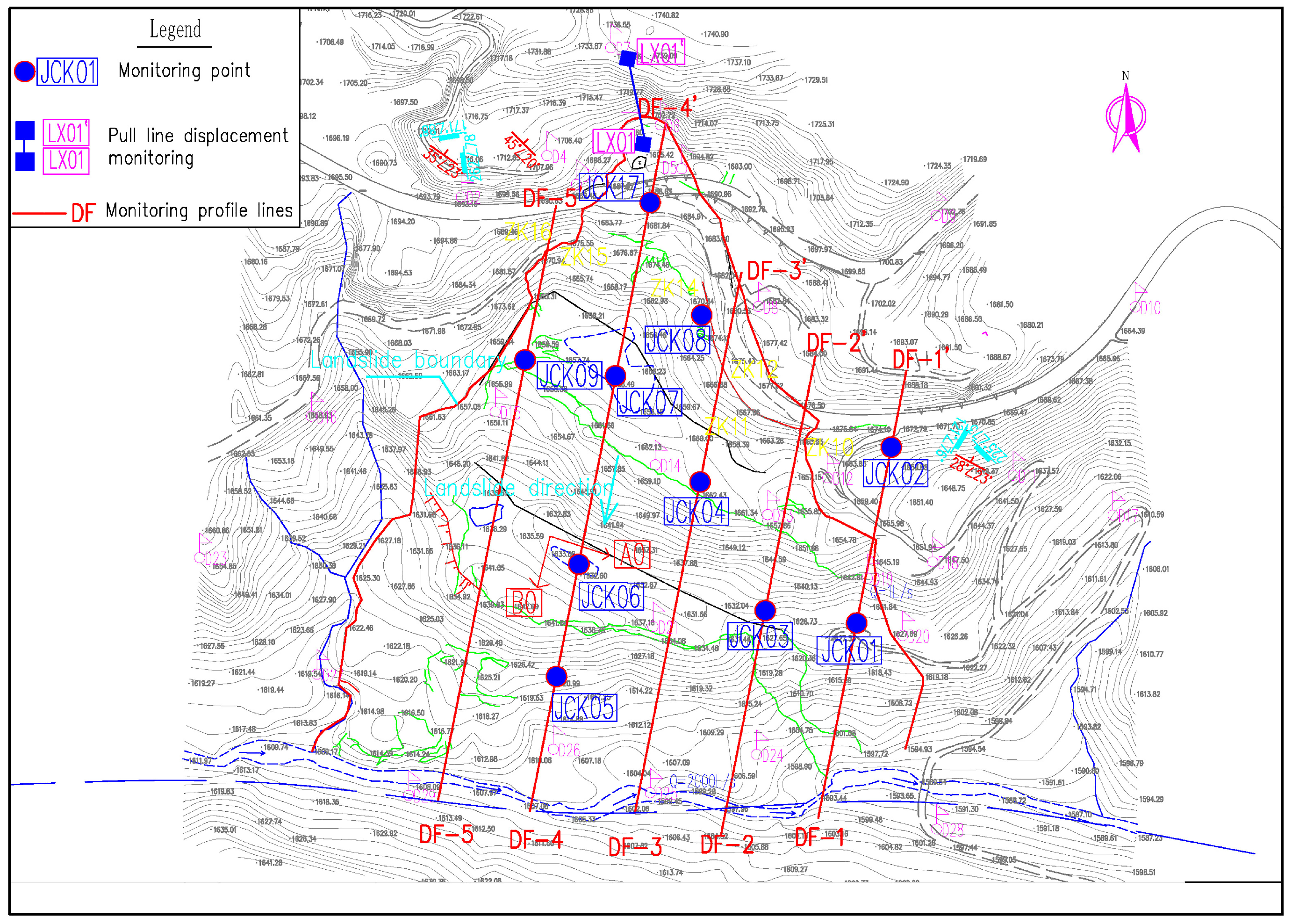
2.2. Slope Monitoring Arrangement

The slope has been experiencing prolonged sliding. In 2019, the local government designated this area as a geological hazard-prone area and installed warning signs to inform the public of the potential danger. Due to heavy rainfall, this slope began to slide again in September 2020. A certain section of the road subgrade was damaged by traction, resulting in large-scale cracking and collapse, which disrupted the road and seriously affected the transportation of villagers. This situation necessitates urgent engineering treatment. To dynamically analyze the deformation characteristics of this landslide, invert the geotechnical mechanical parameters of the landslide, and provide a parameter basis for subsequent emergency rescue work, surface displacement monitoring, deep displacement monitoring, and rainfall monitoring were conducted on this landslide. The detailed monitoring layout is shown in Table 2.
During the monitoring period, ground surface inspections were conducted once a month. In the rainy season, or when abnormalities occurred or deformation intensified, the monitoring frequency increased based on the actual situation. Manual monitoring was conducted 1–4 times per month, with increased frequency during the rainy season, or when abnormalities occurred or deformation intensified. Automatic monitoring was dynamically adjusted in real time based on construction and geological disaster site conditions. The schematic diagram of the monitoring plan is shown in Figure 4.

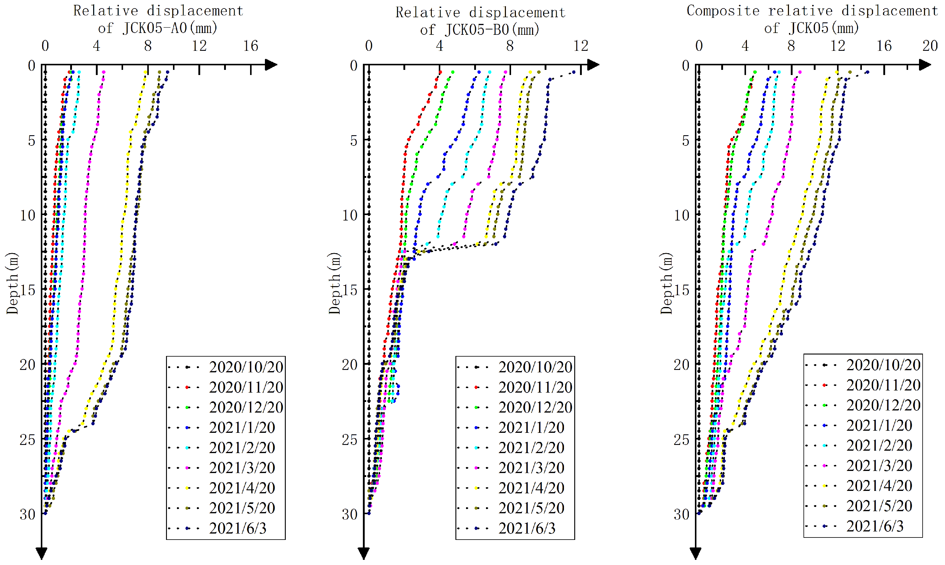
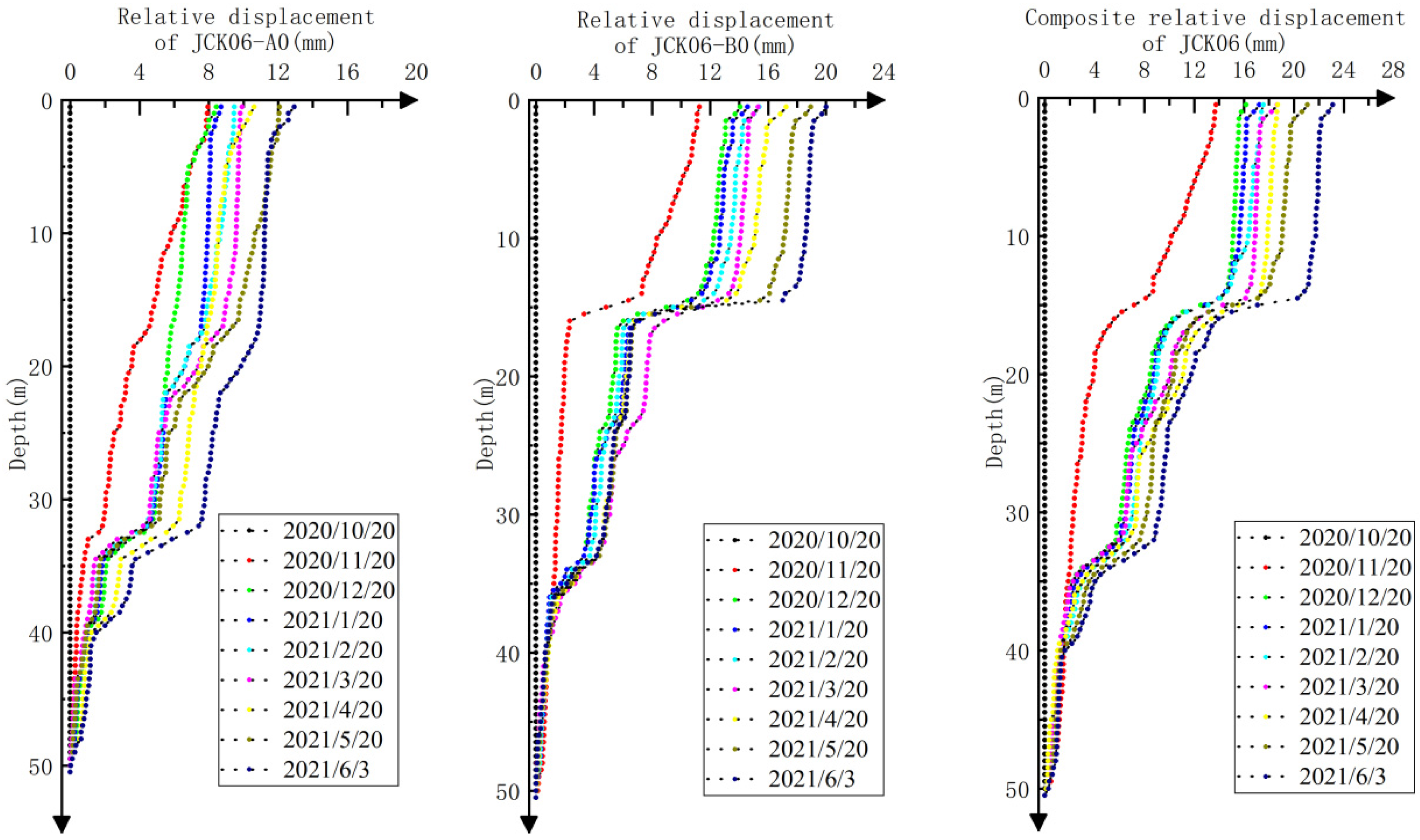
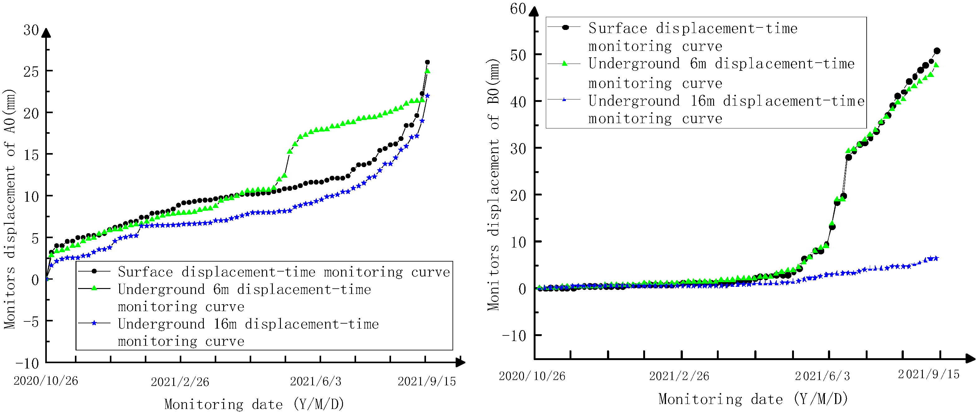
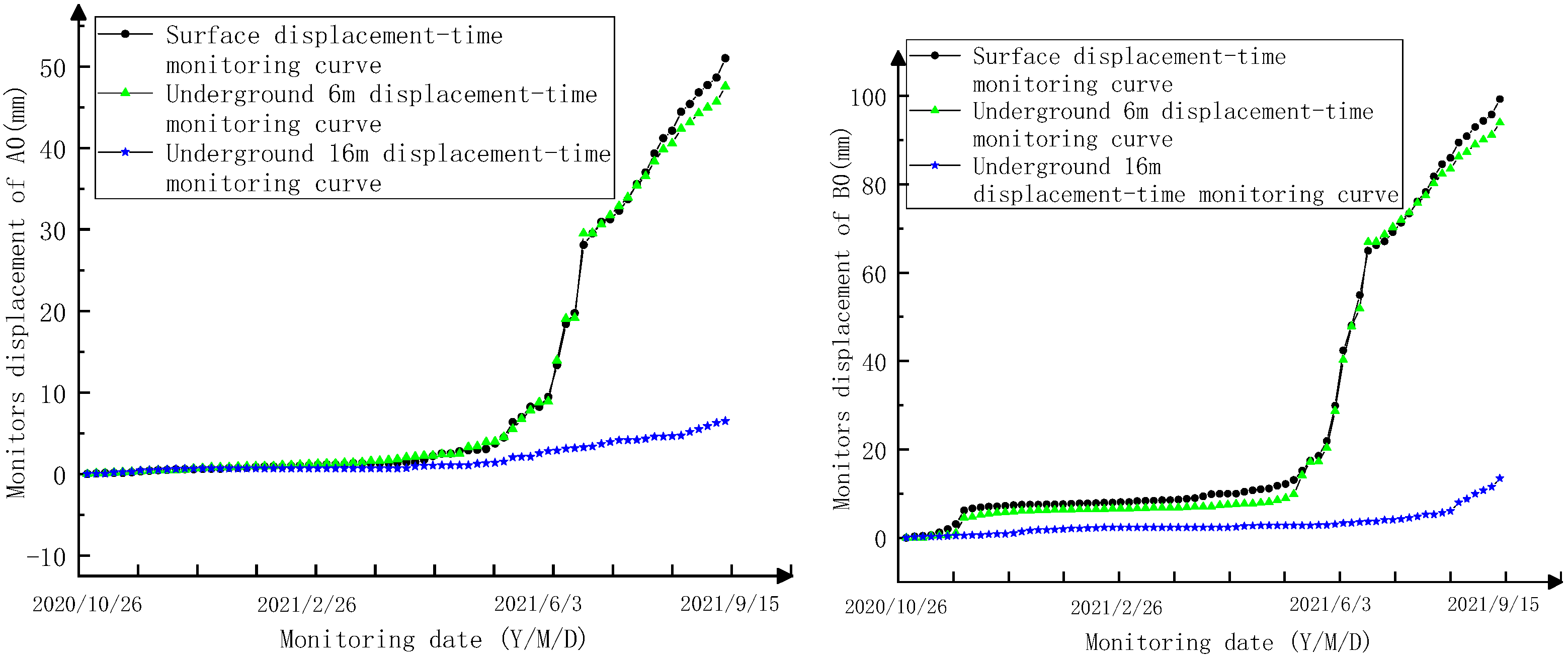
2.3. Analysis of Monitoring Data

This slope began to slide again in September 2020 due to rainfall. After installing and debugging the monitoring equipment, data collection commenced in October 2020. To avoid the impact of on-site construction on the monitoring data, this study used data collected from October 2020 to June 2021, before the start of construction, for analysis.
This slope has five survey lines, with DF4-DF4′ being the main sliding direction survey line. This survey line includes four monitoring boreholes: JCK05, JCK06, JCK07, and JCK17. Additionally, JCK08 is a monitoring borehole along the road. Based on the monitoring data, significant changes were observed at these five monitoring points. Therefore, the data from these five monitoring points were selected to plot the monitoring curves, facilitating the analysis of the slope deformation pattern. The monitoring directions are divided into B0 and A0, with B0 representing the main sliding direction and A0 representing the direction perpendicular to B0. As of 3 June 2021, the monitoring curves for each monitoring borehole are shown in Figure 5, Figure 6, Figure 7, Figure 8 and Figure 9.
Based on the analysis of the monitoring curves, significant inflection points are observed in the monitoring curves of the five monitoring points in the B0 direction (main sliding direction). The depths corresponding to JCK05, JCK06, JCK07, JCK08, and JCK17 are 13.0, 15.5, 16.5, 8.0, and 12.5 m, respectively. This indicates that the sliding surface primarily lies within the depth range of 13 m to 15 m below the ground surface.
From the monitoring curve for JCK08, significant inflection points are observed in the B0 direction, A0 direction, and the combined displacement direction. For JCK07 and JCK17, significant inflection points are observed in both the B0 direction and the combined displacement direction, while no apparent inflection point is observed in the A0 direction. JCK05 exhibits an inflection point only in the monitoring curve for the B0 direction, with no significant changes in the other two curves. For JCK06, the displacement inflection points occur at two depths, namely 15.5 and 34 m. However, the inflection point at 34 m is not prominent. Considering the monitoring curves of the other points, the 34 m depth may correspond to the location of a localized sliding surface.
A comprehensive analysis of the monitoring data reveals that from late October 2020 to early June 2021, the landslide experienced a slow deformation phase due to continuous heavy rainfall. However, from May 2021 to June 2021, there was an increase in the displacement rate, indicating an acceleration in the deformation of the landslide. This suggests a possibility that the landslide may subsequently enter an accelerated deformation phase.

3. Back Analysis of Slope Mechanical Parameters

Based on the monitoring results from Section 2, it is evident that the slope is on the verge of entering an accelerated deformation phase. To ensure safety, conduct a quantitative analysis of slope stability, and provide parameter-based support for landslide remediation measures, it is crucial to accurately determine the geomechanical parameters of the slope. However, due to the specific conditions of the slope during the accelerated deformation phase, it may not be feasible to determine the geomechanical parameters through conventional methods such as surveying, sampling, and testing. The establishment of the parameter inversion analysis model was elaborated in our previous study [42]. Here, we further investigate the key parameters of the inversion model to enhance its accuracy.

3.1. Parameter Research of Inversion Model

Based on previous research findings, the establishment of the parameter inversion analysis model comprises two parts: the objective function acquisition model and the improved NSGA-II algorithm model. The improved BPGA-NSGA-II model, built upon these two components, enables the acquisition of slope mechanical parameter combinations with relatively small relative errors. However, several key issues still require further research regarding the application of the model. Two key aspects that require further investigation are the topology structure of the BP neural network model and the selection of population size and iteration count for the NSGA-II algorithm. These parameters are closely related to the inversion error and directly affect the accuracy of quantitative analysis of slope dynamic stability. Many scholars have done relevant research on how to determine the topological structure of the BP neural network model [43], which will not be introduced in detail in this article. This paper only studies in detail how to determine the key parameters of the NSGA-II algorithm model.
The size of the initial population in the NSGA-II algorithm reflects the diversity of initial solutions. A large initial population can lead to an increase in redundant data and slow down computational speed, while a small initial population may result in a decrease in the accuracy of the Pareto front. Similarly, the number of iterations determines the generations of evolution. If the number of iterations is too high, it can lead to excessively long computation times. Conversely, if the number of iterations is too low, it may not be sufficient to evolve the optimal solution that meets the desired accuracy requirements. Thus, configuring the population size and number of iterations is crucial for the algorithm.
This study employs the controlled variable method to investigate the individual effects of population size and number of iterations on the Pareto solutions. Given that conducting several trial calculations is necessary, the number of monitoring points does not significantly affect the variation pattern of Pareto solutions. However, it can significantly decrease computational speed. Therefore, in this study, only the error functions of three selected monitoring points were used as objective functions [42]. First, the initial population size was set to 100 and the number of iterations to 50. After each iteration, the mean value of the objective function corresponding to the Pareto frontier was recorded and plotted, as shown in Figure 10.
As shown in Figure 10, when the number of iterations is less than 15, both objective functions tend to converge rapidly. When the number of iterations is between 15 and 32, the changes in the values of objective functions F1 and F2 tend to be stable. The rate of change for F1 is lower, showing a slight overall increasing trend. On the other hand, F2 exhibits a decreasing trend initially, followed by an increasing trend. When the number of iterations reaches 33, both F1 and F2 experience a minor mutation. However, as the number of iterations increases, F1 stabilizes, with its value remaining between 1.2 and 1.4. Objective function F2 exhibits slight fluctuations, with values fluctuating between 0.038 and 0.048, but the magnitude of these fluctuations is small. Considering all factors, the number of iterations was set to 45.
On the basis of determining the number of iterations, further research is required on the initial population size. With 45 iterations, the solving process must be repeated 45 times. A large initial population size ensures the diversity of initial solutions but results in longer computation times. Figure 10 shows that there is a brief plateau period when the number of iterations is between 24 and 27. Therefore, we set the number of iterations to 25 to study the variation patterns of the Pareto front under different initial population sizes. We set the initial population size to 10, increasing it by increments of 5 until reaching a population size of 120. The results are shown in Figure 11.
Figure 11 shows that when the population size is less than 70, the fluctuation range of both objective functions, F1 and F2, is significantly large. This is mainly because the initial population is randomly generated and the sample size is small, leading to high randomness in the results. When the population size is between 70 and 100, the fluctuations in the objective function values decrease and tend to stabilize overall. However, there is still a large mutation when the population size is between 90 and 95. When the population size exceeds 100, the fluctuations in the objective function values become minimal. Specifically, F1 stabilizes around 2.3, and F2 stabilizes around 0.4. Therefore, we set the population size to 120 to ensure both calculation speed and the diversity of initial solutions.

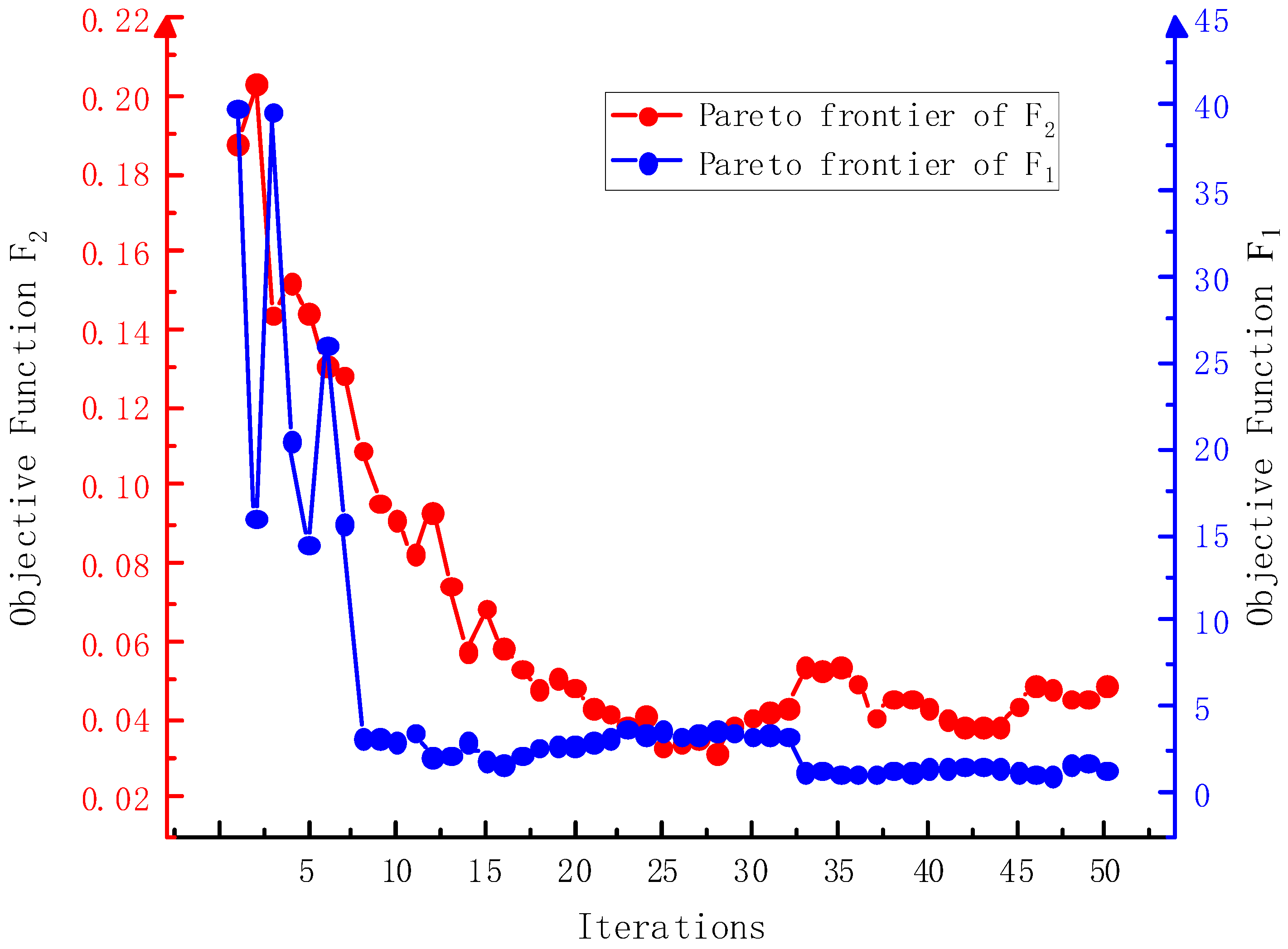
3.2. Inversion of Slope Mechanical Parameters

Compared to our previous model [42], this study adjusted the initial population size. The improved calculation results are compared with the original results, as shown in Figure 12.
It is evident from Figure 12 that after the initial population size is modified, the middle solution of the Pareto front moves forward, resulting in a better solution than before parameter optimization. To facilitate the quantitative analysis of slope dynamic stability, 67 groups of solutions from the Pareto front after parameter improvements were extracted. After performing the denormalization operation and calculating the mean, the parameter combination shown in Table 3 was obtained.

4. Slope Dynamic Stability Analysis

Continuous changes in the external environment inevitably led to dynamic variations in slope stability. Since monitoring data is time-sensitive, the geotechnical parameters obtained through inversion of this data also exhibit time-dependent effects. In this section, we analyze the stability of the slope over different periods using the inverted parameters. The analysis results were validated against actual monitoring data curves, enabling a dynamic assessment of slope stability.

4.1. Slope Stability Calculation

4.1.1. Calculation of Initial Slope Stability

According to the original survey results, the slope strata can be divided into quaternary deposits, weathered layer, moderately weathered sandstone with mudstone and moderately weathered basalt. The calculation parameters for the initial stability of the slope were set according to laboratory test results, as presented in Table 4.
After achieving initial equilibrium, the minimum safety factor of the slope in its natural state was determined to be 1.212, indicating that the slope is in a stable condition. To provide a more visual representation of the safety factor of the three-dimensional slope, the safety factor was extracted using the Fish function and displayed as a cloud map, as shown in Figure 13. The figure shows that the slope exhibits a minimum safety factor of 1.212 and a maximum safety factor of 1.737.
Following a heavy rainfall event in September 2020, the slope showed signs of sliding. Therefore, calculations were conducted to assess the stability of the slope after the rainfall event. The simulated rainfall scenario involved two components of fluid–soil coupling. The first component pertains to the region below the groundwater level, which is already in a saturated state. The second component relates to the region above the groundwater level, where fluid–soil coupling occurs due to rainfall infiltration. For the region below the groundwater level, the fluid–soil coupling was achieved by altering the pore water pressure based on the given groundwater table position. For the region above the groundwater level, which predominantly consists of fourth-grade coarse-grained soil, the infiltration process occurs rapidly. Therefore, a strength reduction method was employed to couple this region. The calculated safety factor cloud map is shown below (Figure 14).
From Figure 14, it is evident that the minimum safety factor of the slope after the rainfall is only 0.954, indicating an unstable condition. The high-risk zone is concentrated in the lower-left area of the landslide region, where all safety factors are less than 1. The boundary of the landslide observed during the survey is consistent with the area depicted in the figure where the safety factor is less than 1.15. This indicates that the landslide was a tensile landslide caused by the instability of the lower area.

4.1.2. Real-Time Slope Stability Analysis

The inversion parameters in Table 3 are the results obtained using the monitoring data of June 2021. The stability of the slope in June 2021 was calculated by substituting the data in Table 2 into the three-dimensional model. After extracting the safety factors of each point, the safety factor cloud map is obtained (Figure 15).

4.2. Slope Dynamic Monitoring

Based on the analysis results in Section 4.1.1, it can be observed that the safety factor of the slope was already around 0.8 in early June 2021, indicating an unstable state. To protect the road, slope remediation was conducted in the upper region of the slope, implementing measures such as the installation of retaining piles. No specific measures were taken for the lower region of the slope. To validate the accuracy of the dynamic slope stability analysis and the reliability of the inverted parameters, further monitoring was conducted in the lower region of the slope at monitoring points JCK06 and JCK07. Monitoring data were collected until 15 September 2021, after which the monitoring hole was sheared off. The monitoring curves are shown in Figure 16 and Figure 17.
From the actual monitoring curves, it is evident that the displacement rates with respect to time significantly increased for JCK06 in the B0 direction and for JCK07 in the A0 and B0 directions after 3 June 2021. For JCK06, the initial stage of displacement increase in the A0 direction was lower compared to the other three directions, but the displacement rate gradually increased in later stages, exhibiting a typical exponential growth trend. These observations are consistent with the results obtained from the slope stability analysis using the inverted parameters. It indicates that the method used for dynamic slope stability analysis is effective.

5. Conclusions

This study focuses on the dynamic stability analysis of highway slopes that have already experienced damage during the operational phase. First, based on the improved BPGA-NSGA-II model, its parameter settings were further studied. Second, the real-time mechanical parameters of the slope were obtained by inversion using the optimized model. Third, slope stability was dynamically analyzed using the inversion results. Finally, the reliability of the calculation results was verified using subsequent field monitoring data. The main conclusions are as follows:

5.1. Research Results

(1) For the objective function of slope establishment, when the population size of the improved NSGA-II algorithm was 120 and the number of iterations was 45, a relatively high inversion accuracy was obtained while ensuring the calculation speed.
(2) The initial stability of the slope and the stability in early June 2021 were calculated, respectively. In the initial state, the slope stability coefficient was calculated at 1.212, indicating a stable state. After being affected by rainfall, the stability coefficient dropped to 0.954, indicating a critical unstable state. In June 2021, the slope stability coefficient was 0.8, confirming an unstable state. Based on this, the dynamic stability analysis of the slope was realized.
(3) The actual displacement monitoring curves of the monitoring points JCK06 and JCK07 revealed that the slope entered an accelerated sliding phase after June 2021. The results are consistent with those of the slope dynamic stability calculations using inversion parameters, validating the reliability of this method in slope dynamic stability analysis.

5.2. Limitations and Future Work Plan

This study focused on refining the parameter setting of the improved BPGA-NSGA-II model and used the improved model to conduct a dynamic analysis of the stability of the case slope. The analysis results were verified using actual monitoring data, confirming the reliability of the model. However, there are notable shortcomings:
(1) This study included a limited number of research cases, warranting further verification to assess the applicability of the method to different slope types;
(2) Research on improving the key parameters of the NSGA-II algorithm is limited by calculation speed. This study was confined to population sizes in the order of 102 and the number of iterations in the order of 101. To establish parameter rules with different numbers of objective functions and different magnitudes, further investigation is required.

Author Contributions

Conceptualization, B.H. and X.D.; methodology, B.H.; software, B.H.; validation, J.Y. and D.M.; formal analysis, X.D.; investigation, M.B.; resources, M.B.; data curation, B.H.; writing—original draft preparation, B.H.; writing—review and editing, B.H.; visualization, B.H.; supervision, X.D.; project administration, J.Y. and D.M.; funding acquisition, M.B. All authors have read and agreed to the published version of the manuscript.

Funding

This research was funded by The National Key Research and Development Project of China, the Ministry of Science and Technology of China (Grant 2018YFC1505504).

Institutional Review Board Statement

Not applicable.

Informed Consent Statement

Not applicable.

Data Availability Statement

The data presented in this study are available on request from the corresponding author. The data are not publicly available due to privacy.

Conflicts of Interest

Authors Jinwen Yang and Dong Ma was employed by the company China Railway 16th Bureau Group Co., Ltd. The remaining authors declare that the research was conducted in the absence of any commercial or financial relationships that could be construed as a potential conflict of interest.

References

  1. Wu, L.L.; He, K.Q.; Guo, L.; Zhang, J.; Sun, L.; Jia, Y. Research on the excavation stability evaluation method of Chaqishan ancient landslide in China. Eng. Fail. Anal. 2022, 141, 106664. [Google Scholar] [CrossRef]
  2. Lin, F.; Wu, L.Z.; Huang, R.Q.; Zhang, H. Formation and Characteristics of the Xiaoba Landslide in Fuquan, Guizhou, China. Landslides 2017, 15, 669–681. [Google Scholar] [CrossRef]
  3. Domínguez-Cuesta, M.J.; Quintana, L.; Valenzuela, P.; Cuervas-Mons, J.; Alonso, J.L.; Cortés, S.G. Evolution of a Human-induced Mass Movement Under the Influence of Rainfall and Soil Moisture. Landslides 2021, 18, 3685–3693. [Google Scholar] [CrossRef]
  4. Nguyen, L.C.; Tien, P.V.; Do, T.N. Deep-seated rainfall-induced landslides on a new expressway: A case study in Vietnam. Landslides 2020, 17, 395–407. [Google Scholar] [CrossRef]
  5. Martino, S.; Bozzano, F.; Caporossi, P.; D’Angiò, D.; Della Seta, M.; Esposito, C.; Fantini, A.; Fiorucci, M.; Giannini, L.M.; Iannucci, R.; et al. Impact of landslides on transportation routes during the 2016–2017 Central Italy seismic sequence. Landslides 2019, 16, 1221–1241. [Google Scholar] [CrossRef]
  6. Deng, E.; Xiang, Q.; Johnny, C.L.C.; Dong, Y.; Tu, S.; Chan, P.-W.; Ni, Y.-Q. Increasing temporal stability of global tropical cyclone precipitation. NPJ Clim. Atmos. Sci. 2025, 8, 11. [Google Scholar] [CrossRef]
  7. Zheng, Y.R. Development and application of numerical limit analysis for geological materials. Chin. J. Rock Mech. Eng. 2012, 31, 1297–1316. [Google Scholar]
  8. Wang, S.Y.; Tong, X.D. Stability analysis of slopes based on dynamic strength reductionimproved vector sum method. Chin. J. Geotech. Eng. 2023, 45, 1384–1392. [Google Scholar]
  9. Zhang, R.H.; Ye, S.H.; Tan, H. Stability analysis of multistage homogeneous loess slopes by improved limit equilibrium method. Rock Soil Mech. 2021, 42, 813–825. [Google Scholar]
  10. Lu, K.L.; Zhu, D.Y.; Gan, W.N. 3D limit equilibrium method for slope stability analysis and its application. Chin. J. Geotech. Eng. 2013, 35, 2276–2282. [Google Scholar]
  11. Liu, Z.P.; Yang, B.; Liu, J.; Ai, F. Three-dimensional limit equilibrium method based on GRASS GIS and TIN sliding surface. Rock Soil Mech. 2017, 38, 221–227. [Google Scholar]
  12. Nandi, S.; Santhoshkumar, G.; Ghosh, P. Development of limiting soil slope profile under seismic condition using slip line theory. Acta Geotech. 2021, 16, 3517–3531. [Google Scholar] [CrossRef]
  13. Bishop, A.W. The use of the slip circle in the stability analysis of slopes. Geotechnique 1955, 5, 7–17. [Google Scholar] [CrossRef]
  14. Flaate, K.; Janbu, N. Soil exploration in a 500 m deep fjord, Western Norway. Mar. Geotechnol. 1975, 1, 117–139. [Google Scholar] [CrossRef]
  15. Spencer, E. A method of analysis of the stability of embankments assuming parallel inter-slice forces. Geotechnique 1967, 17, 11–26. [Google Scholar] [CrossRef]
  16. Singh, J.; Verma, A.K.; Banka, H. Application of Biogeography based optimization to locate critical slip surface in slope stability evaluation. In Proceedings of the 4th International Conference on Recent Advances in Information Technology, Dhanbad, India, 15–17 March 2018; pp. 1–5. [Google Scholar]
  17. Meng, J.; Huang, J.; Sloan, S.W.; Sheng, D. Discrete modelling jointed rock slopes using mathematical programming methods. Comput. Geotech. 2018, 96, 189–202. [Google Scholar] [CrossRef]
  18. Chen, J.G.; Li, H.; He, Z.Y. Homogeneous soil slope stability analysis based on variational method. Rock Soil Mech. 2019, 40, 2931–2937. [Google Scholar]
  19. Zhou, X.P.; Huang, X.C.; Zhao, X.F. Optimization of the Critical Slip Surface of Three-Dimensional Slope by Using an Improved Genetic Algorithm. Int. J. Geomech 2020, 20, 04020120. [Google Scholar] [CrossRef]
  20. Zhou, F.X.; Zhu, S.W.; Liang, Y.W.; Zhao, W. Exact analysis of soil slope stability by using variational limit equilibrium method. Chin. J. Geotech. Eng. 2023, 45, 1341–1346. [Google Scholar]
  21. Lu, R.L.; Wei, W.; Shang, K.W.; Jing, X. Stability Analysis of Jointed Rock Slope by Strength Reduction Technique considering Ubiquitous Joint Model. Adv. Civ. Eng. 2020, 2020, 8862243. [Google Scholar] [CrossRef]
  22. Renani, H.R.; Martin, C.D. Factor of safety of strain-softening slopes. J. Rock Mech. Geotech. Eng. 2020, 12, 473–483. [Google Scholar] [CrossRef]
  23. Sengani, F.; Allopi, D. Accuracy of Two-Dimensional Limit Equilibrium Methods in Predicting Stability of Homogenous Road-Cut Slopes. Sustainability 2022, 14, 3872. [Google Scholar] [CrossRef]
  24. Zienkiewicz, O.C.; Humpheson, C.; Lewis, R.W. Associated and non-associated visco-plasticity and plasticity in soil mechanics. Geotechnique 1975, 25, 671–689. [Google Scholar] [CrossRef]
  25. Renani, H.R.; Martin, C.D.; Varona, P.; Lorig, L. Stability analysis of slopes with spatially variable strength properties. Rock Mech. Rock Eng. 2019, 52, 3791–3808. [Google Scholar] [CrossRef]
  26. Zhou, Y.; Cheng, X.H. High fill slope collapse: Stability evaluation based on finite element limit analyses. Transp. Geotech. 2024, 44, 101156. [Google Scholar]
  27. Sourav, S.; Manash, C. Stability analysis for two-layered slopes by using the strength reduction method. Int. J. Geo-Eng. 2021, 12, 24. [Google Scholar]
  28. Feng, S.; Zhao, Y.; Li, B.Y.; Wu, K. A Calculation Method of Double Strength Reduction for Layered Slope Based on the Reduction of Water Content Intensity. Comput. Model. Eng. Sci. 2024, 138, 221–243. [Google Scholar]
  29. Yu, M.D. Analysis on stability of mountain mass and numerical calculation of landslide resistance based on strength reduction method. Arab. J. Geosci. 2020, 13, 617. [Google Scholar] [CrossRef]
  30. Tayebeh, K.; Mohammad, R.A. Three-dimensional stability of locally loaded geocell-reinforced slopes by strength reduction method. Geomech. Geoengin.-Int. J. 2019, 14, 1581275. [Google Scholar]
  31. Hua, C.Y.; Yao, L.H.; Song, C.G.; Ni, Q.; Chen, D. A New Criterion for Defining Inhomogeneous Slope Failure Using the Strength Reduction Method. Comput. Model. Eng. Sci. 2022, 132, 413–434. [Google Scholar] [CrossRef]
  32. Du, Y.; Xie, M.W.; Lv, F.X.; Wang, Z.; Wang, G.; Liu, Q. New method for dynamic analysis of rock slope stability based on modal parameters. Chin. J. Geotech. Eng. 2015, 37, 1334–1339. [Google Scholar]
  33. Wang, C.; Zhang, R.R.; Zhang, F.H.; Du, C. A dynamic simulation analysis method of high-steep slopes based on real-time numerical model and its applications. Chin. J. Geotech. Eng. 2016, 37, 2383–2390. [Google Scholar]
  34. Song, L.F.; Xu, B.; Kong, X.J.; Zou, D.; Pang, R.; Yu, X.; Zhang, Z. Three-dimensional slope dynamic stability reliability assessment based on the probability density evolution method. Soil Dyn. Earthq. Eng. 2019, 120, 360–368. [Google Scholar] [CrossRef]
  35. Liu, H.Y.; Bai, M.Z.; Li, Y.J.; Yang, L.; Shi, H.; Gao, X.; Qi, Y. Landslide displacement prediction model based on multisource monitoring data fusion. Measurement 2024, 236, 115055. [Google Scholar] [CrossRef]
  36. Xiao, H.P.; Guo, G.L.; Chen, L.L. Research on Dynamic Evaluation Model of Slope Risk Based on Improved VW-UM. Math. Probl. Eng. 2019, 2019, 5813217. [Google Scholar] [CrossRef]
  37. Ai, Z.B.; Zhang, H.L.; Wu, S.C.; Jiang, C.; Yan, Q.; Ren, Z. Study on the slope dynamic stability considering the progressive failure of the slip surface under earthquake. Front. Earth Sci. 2022, 10, 981503. [Google Scholar] [CrossRef]
  38. Wu, J.; Guo, D.Y.; Zhang, L.W.; Wang, L. Stability analysis of arch dam and slope of the Xiluodu hydropower station on the Jinsha river. Chin. J. Rock Mech. Eng. 2023, 42, 2478–2494. [Google Scholar]
  39. Qu, X.L.; Chen, J.; Tang, H.; Dong, R.; Qi, C. Rock slope dynamic stability analysis based on coupling temporal domain numerical manifold method. Chin. J. Rock Mech. Eng. 2022, 41, 82–91. [Google Scholar]
  40. Wang, W.; Yang, Y.; Yang, X.; Gayah, V.V.; Wang, Y.; Tang, J.; Yuan, Z. A Negative Binomial Lindley Approach Considering Spatiotemporal Effects for Modeling Traffic Crash Frequency with Excess Zeros. Accid. Anal. Prev. 2024, 207, 107741. [Google Scholar] [CrossRef]
  41. Yang, Y.; Yin, Y.X.; Wang, Y.P.; Meng, R.; Yuan, Z. Modeling of Freeway Real-Time Traffic Crash Risk Based on Dynamic Traffic Flow Considering Temporal Effect Difference. J. Transp. Eng. Part A Syst. 2023, 149, 04023063. [Google Scholar] [CrossRef]
  42. He, B.H.; Du, X.L.; Bai, M.Z.; Yang, J.-W.; Ma, D. Inverse analysis of geotechnical parameters using an improved version of non-dominated sorting genetic algorithm II. Comput. Geotech. 2024, 171, 106416. [Google Scholar] [CrossRef]
  43. Baum, E.B.; Haussler, D. What size net gives valid generalization? Neural Comput. 1989, 1, 151–160. [Google Scholar] [CrossRef]
Figure 1. Landslide along the Zhaoping-Pingle.
Applsci 15 06914 g001
Figure 2. Kinnaur high-velocity landslide, Himachal Pradesh.
Applsci 15 06914 g002
Figure 3. Landslide map.
Applsci 15 06914 g003
Figure 4. Schematic monitoring floor plan of the Yama Line, China, landslide [42].
Applsci 15 06914 g004
Figure 5. Monitoring curve results for JCK05 monitoring hole.
Applsci 15 06914 g005
Figure 6. Monitoring curve results for JCK06 monitoring hole.
Applsci 15 06914 g006
Figure 7. Monitoring curve results for JCK07 monitoring hole.
Applsci 15 06914 g007
Figure 8. Monitoring curve results for JCK08 monitoring hole.
Applsci 15 06914 g008
Figure 9. Monitoring curve results for JCK17 monitoring hole.
Applsci 15 06914 g009
Figure 10. Trend graph of the objective function changing with the number of iterations.
Applsci 15 06914 g010
Figure 11. Trend diagram of objective function variation with population size.
Applsci 15 06914 g011
Figure 12. Pareto frontier comparison chart before and after model improvement.
Applsci 15 06914 g012
Figure 13. Cloud map of initial slope safety factor.
Applsci 15 06914 g013
Figure 14. Safety factor cloud map after rainfall.
Applsci 15 06914 g014
Figure 15. Real-time cloud map of safety factor for slope.
Applsci 15 06914 g015
Figure 16. Displacement monitoring data for JCK06.
Applsci 15 06914 g016
Figure 17. Displacement monitoring data for JCK07.
Applsci 15 06914 g017
Table 1. Test table of rock and soil mechanical parameters.
Serial NumberStratumRock TypeThickness (m)
1 Q 4 m Quaternary artificial fill2~6.5
2 Q 4 c Quaternary collapse accumulation layer block stone soil3.1~23
3 Q 4 e l + d l Quaternary residual slope deposit silty clay1.7~9.3
4 P 3 l Sandstone with mudstone3.3~10.5
5 P 3 β Basalt9.2~20
Table 2. Summary of planned monitoring workload.
Monitoring ProjectPoint NumberHole Depth (m)Total (m)
Deep displacement monitoringJCK0128312.5
JCK0216
JCK0333
JCK0433
JCK0529.5
JCK0650
JCK0735
JCK0829.5
JCK0930
JCK1728.5
Surface displacement monitoring1 set of surface pull-wire intelligent displacement meter
Rainfall monitoring1
Surface patrolOnce a month, with more frequent patrols during the rainy season
Table 3. Inversion results of mechanical parameters of each model.
LayerQuaternary DepositsWeathered LayerInterbedded Sandstone and Shale LayerModerately Weathered Basalt Layer
ParameterY1C1 φ 1 Y2C2 φ 2 Y3C3 φ 3 Y4C4 φ 4
UnitMPakPa°MPakPa°GPakPa°GPakPa°
Original value32.819.730.319.323.123.430.653.929.964.276.242.6
Improved value31.916.929.518.433.417.442.355.235.370.775.432.1
Table 4. Model calculation parameter table.
LayerDensity (kg/m3)Young’s Modulus (kPa)Poisson’s RatioCohesion (kPa)Internal Friction Angle (°)
Quaternary deposits1850.002.00 × 1040.3023.0024.00
Weathered layer2200.001.00 × 1060.2840.0015.00
Moderately weathered sandstone with mudstone2300.003.00 × 1070.2570.0035.00
Moderately weathered basalt2900.004.00 × 1070.2075.0055.00
Disclaimer/Publisher’s Note: The statements, opinions and data contained in all publications are solely those of the individual author(s) and contributor(s) and not of MDPI and/or the editor(s). MDPI and/or the editor(s) disclaim responsibility for any injury to people or property resulting from any ideas, methods, instructions or products referred to in the content.

