Article

HRR-Based Calibration of an FDS Model for Office Fire Simulations Using Full-Scale Wood Crib Experiments

1
CAMBI Research Center and Doctoral School, Faculty of Building Services Engineering, Technical University of Civil Engineering of Bucharest, 020396 Bucharest, Romania
2
Fire Officers Faculty, Police Academy, 022451 Bucharest, Romania
*
Author to whom correspondence should be addressed.
Appl. Sci. 2025, 15(12), 6909; https://doi.org/10.3390/app15126909
Submission received: 26 May 2025 / Revised: 11 June 2025 / Accepted: 17 June 2025 / Published: 19 June 2025
(This article belongs to the Special Issue Recent Advances and Emerging Trends in Computational Fluid Dynamics)

Abstract

This study deals with the simulation of office fires by combining large-scale experiments with nine wooden cribs and a carefully calibrated computer model. It shows how real fire conditions, reaching up to 800–1000 °C, could be reproduced experimentally. The numerical model was validated by comparing HRR and temperature data with real measurements. Accuracy was assessed using error metrics to ensure that the simulation closely approximates real fire behavior. The method of determining HRR through mass loss has been used in prior studies, but those typically involved small-scale setups and limited fire loads. Unlike most approaches in the field, this research is based on a full-scale experiment involving nine wooden cribs, offering superior realism and thermal intensity. The experimental data—temperature evolution, HRR, and observed destructive effects—were used to calibrate the FDS model. The strength of the study lies in the repeatability and accuracy of the simulation, its practical relevance, and its potential to improve fire safety evaluations for office spaces.

1. Introduction

In the last two decades, the size of spaces has considerably decreased, leading to a reduced area allocated per user, with constructions not aimed at space optimization becoming increasingly rare. In office spaces, this area has shrunk significantly, reaching values of 19.5 m2 in the European Union and 16 m2 in the United States [1], and sometimes even lower. This trend has resulted in a continuous increase in demand for office spaces, a phenomenon that is evident in cities such as Bucharest, where the demand has grown by approximately 75% from 2012 to the present [2]. In this context, the outbreak of a fire in an office becomes not only a plausible scenario but a major concern for building safety and occupant protection.
Fires continue to represent the primary cause of emergency situations, with severe effects on both people and property. Although advances in fire safety have led to reduced risks across various types of buildings, new architectural configurations and modern interior design materials—especially plastics—have increased the danger by amplifying the emission of toxic gases (CO, CO2) and reducing visibility [3,4,5,6,7]. As a result, understanding fire dynamics remains a top priority for research.
Heat Release Rate (HRR) is a central parameter in fire behavior analysis, reflecting combustion intensity, temperature evolution, toxic gas generation, and flame propagation. HRR has a key role in assessing thermal conditions within a fire-affected compartment and in calibrating advanced numerical models (CFDs). Without an accurate characterization of HRR, estimates related to fire safety, ventilation, or evacuation can become unreliable in real-life scenarios [8]. Without an accurate characterization of HRR, estimates related to fire safety, ventilation, or evacuation can become unreliable in real-life scenarios.
In the specialized literature, the use of standardized temperature–time curves—such as ISO—developed under laboratory conditions, with simplified geometries and limited fuel quantities, is a common practice [9,10,11]. Although useful for material testing, these models fail to capture the complex behavior of real fires, particularly in office buildings that typically feature open layouts, modern furnishings, and a high load of synthetic combustibles [12,13,14]. Recent studies have experimented with determining the heat release rate (HRR) through mass loss methods, as referenced in [15,16,17,18,19,20,21,22], typically focusing on simplified scenarios with small-scale fire sources and reduced thermal loads. Full-scale experimental studies, especially for office-type fires, are extremely rare or lacking entirely, creating a significant knowledge gap in terms of how real fires behave in such environments and how accurately simulation models can capture this behavior.
This paper aims to close that gap by conducting a full-scale fire experiment in an office setting, generating rare and high-fidelity data used to calibrate and validate a Fire Dynamics Simulator (FDS) model. The originality of the research lies in combining robust experimental results with detailed numerical modeling to closely replicate temperature distributions and HRR evolution under real conditions. By doing so, the study not only advances the field with a rare and reproducible validation dataset but also proposes an integrated, interdisciplinary framework that overcomes the limitations of current standard-based approaches and enhances the practical reliability of fire simulations in modern administrative buildings.
In this context, the current study aims to address an office fire through an experimental study to determine the real fire curve, using wood cribs as a fuel source, in a full-scale experimental stand. The results obtained will be useful not only for understanding the thermal behavior of fires but also for validating numerical simulations and underlining more efficient fire protection technical solutions tailored to modern construction requirements, ultimately providing, alongside the characteristics of the fire source (HRR evolution), the refinement of the simulation domain cell (mesh).
The current research framework offers promising applications for analyzing structures exposed to fire, particularly in the context of multi-story buildings. The adaptation of our numerical model can be extended to assess structural fire resistance, as demonstrated in [23], providing valuable insights into the resilience of building materials under high-temperature conditions. Moreover, as study [24] suggests, scaling our model to larger buildings tackles fire safety challenges in structures with many more occupants. Next, we present the experimental set-up, results, numerical model development, numerical results, and calibration phase, demonstrating the model’s potential for safer, more resilient environments.

2. Experimental Set-Up

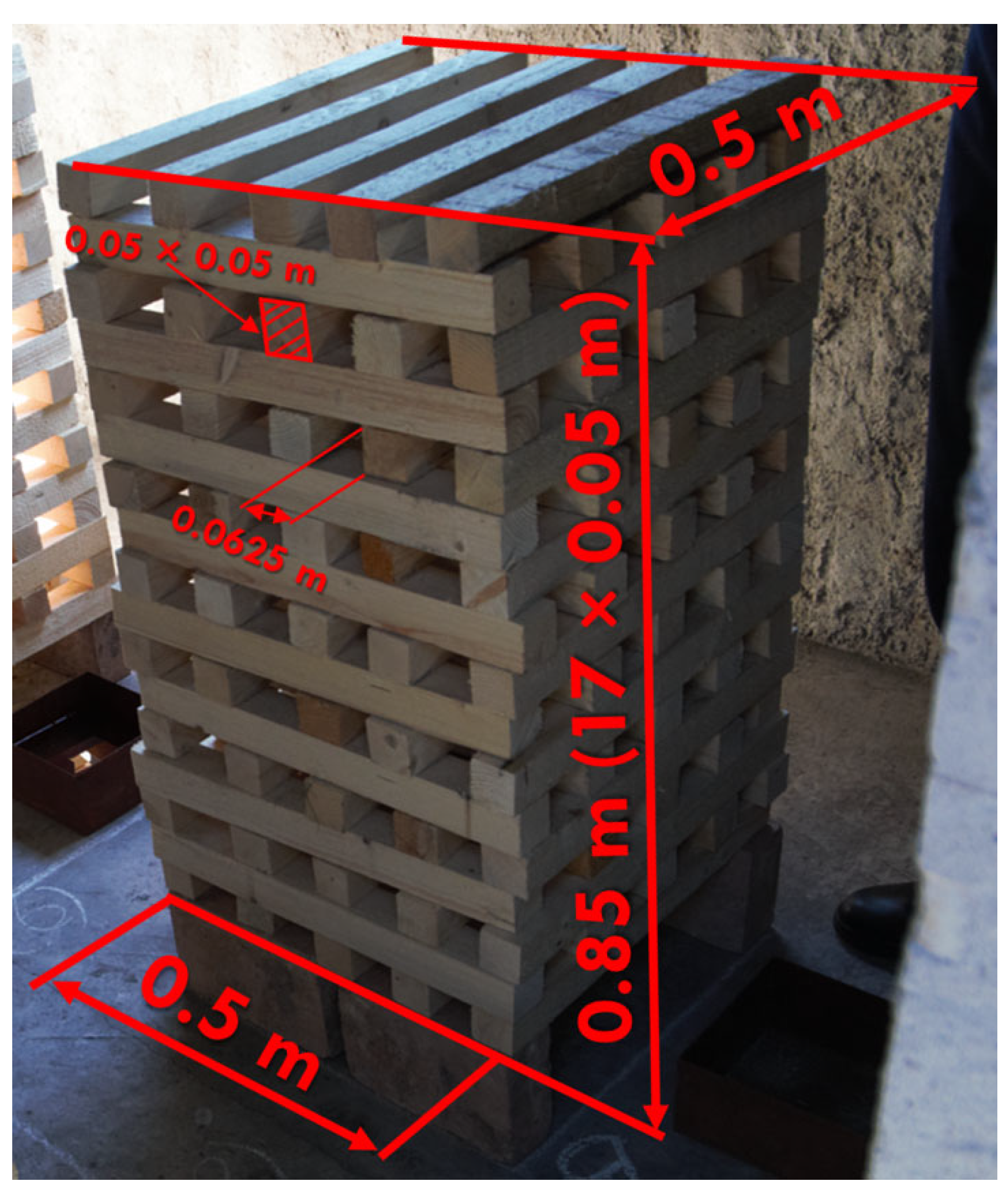
2.1. Scaling Strategy and Crib Configuration

Wood cribs are utilized to replicate the fire source in experiments. One of the advantages of wood cribs is their ability to release thermal energy in an inconsistent yet prolonged manner throughout the experiment, keeping the fire in an active burning phase. This behavior accurately reflects the real evolution of a fire in terms of HRR and temperature over time [25,26]. Unlike a fluid-aggregate fuel source, wood cribs exhibit more pronounced development due to their significantly larger combustion surface area relative to the same thermal load. Therefore, to achieve feasible results, a clear definition of the wood crib configuration [27] is necessary through full-scale testing in room-sized stands, conforming to specific guidelines [28].
The objective of this work is to experimentally replicate the destructive effects of an office fire and measure the interior temperatures to which the occupants might be exposed. According to the referenced standard [29], the density of the thermal load is 420 MJ/m2. A full-scale experimental stand with a usable area of 16 m2 was utilized, built as part of a research program. Using a specialized program [27], designed in compliance with standard [28], a theoretical HRR generated by burning a crib of a specific configuration was determined. The configuration of the wood crib has a significant influence on the final HRR value. According to the reference [27], this configuration involves defining several input parameters, as shown in Figure 1:
-
cross-section of the wood stick (D2);
-
spacing between sticks (S);
-
crib height (hC);
-
number of sticks per row (n);
-
ventilated area (Av);
-
height of the ventilated area (hv);
-
initial mass of the crib (m0);
-
heat of combustion (HU).
The HRR value is directly proportional to the calorific power of the combustible material and the mass loss rate. In our experiment, this calculation included both the ethanol and stack components, with adjustments made to account for ethanol’s minor caloric impact. By integrating HRR over time, we obtained the total thermal energy released during combustion, expressed in kJ, and ensured accuracy despite challenges such as data discontinuities caused by partial or total stack collapse. These corrections allowed for a precise experimental determination of the cumulative heat release rate.
To determine the HRR evolution for an office fire with a source constituted by nine cribs, as depicted in Figure 1, a preliminary controlled full-scale experiment with a single crib was necessary. This experiment allowed for the monitoring of the fuel’s mass loss, and hence the HRR, as well as the temperature inside the stand (as shown in Figure 2a,b). This was made possible by significantly lower temperatures, which permitted the use of a thermally insulated scale capable of withstanding the conditions during combustion. Referring to similar studies in the field [27,30], the single-crib experiment [31] determined an experimental HRR value of a 745 MJ fire.
Considering that the specific heat of combustion of the fuel material remains constant, and the temperature evolution does not follow a direct proportionality with the HRR but rather a dependence characterized by HRR^(2/3), as described in reference [32], measuring the temperature in the experiment involving nine cribs provides a valid benchmark for estimating the HRR value. Since the total mass of fuel can be proportionally scaled with the number of cribs, it was possible to extrapolate the HRR evolution for this extended configuration (Figure 2c), thereby creating the conditions for conducting an experiment with a wood quantity nine times greater to correspond to an office fire with a thermal load of 6720 MJ, in compliance with current standards [11].
The number of cribs was determined by dividing the thermal load by the heat of combustion of the wood, 17.5 MJ/kg [11], resulting in 384 kg of pine wood with minimal moisture. Initially, the wood moisture content was 35%, but it was reduced to 12% using a controlled drying process, where the wooden bars were placed in a hot air chamber for seven days, and measured with a moisture meter. From a total of 1000 wooden bars, 768 were selected to meet strict criteria for weight, volume, and moisture content. Each bar was individually weighed to approximately 0.5 kg, with a maximum error margin of 25 g, ensuring uniformity in wood composition and promoting homogenous combustion characteristics. Understanding the critical effects of wood’s consistency and moisture on pyrolysis and combustion dynamics, this meticulous selection process was essentially to minimize variability and ensure reliable experimental conditions.
In addition to data obtained from direct measurements, this study will also employ the program described in reference [27], which allows for the comparison of experimentally determined values with theoretical ones. This dual approach provides an additional level of validation for the results, reinforcing the feasibility of the proposed methodology. The experiment thus becomes more relevant not only for understanding the phenomenon under study but also as a useful reference for future research or engineering applications in the field of fire safety.

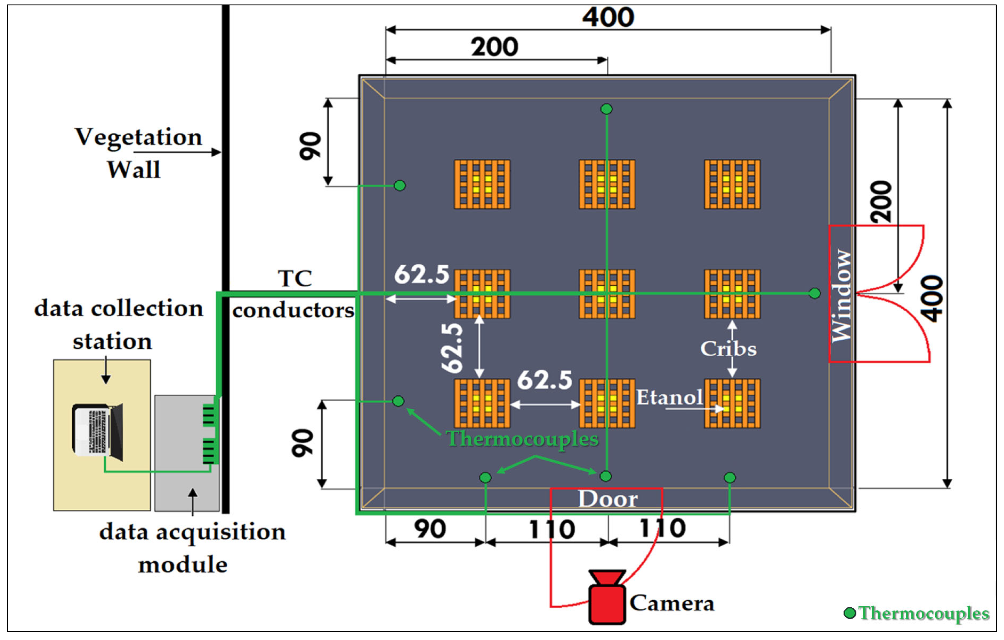
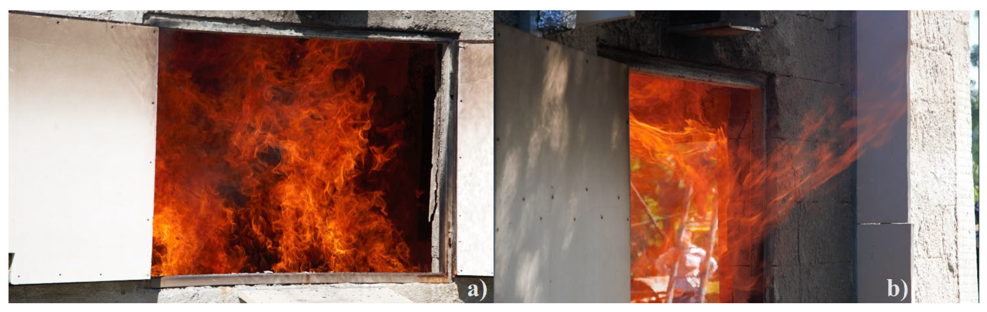
2.2. Experimental Stand

The office fire reproduction experiment was conducted within a full-scale stand with a usable area of 16 m2 (Figure 2), constructed as part of the research program by doctoral student Mihai Dima. The experimental stand features a 2 m2 door and two steel-framed windows, each with an area of 1.4 m2, thermally protected with internal coverings of non-combustible insulation materials, namely basalt wool and calcium silicate. The chosen ventilation scenario involved keeping just the window opposite the door closed. On the exterior, the glass of the windows was replaced with 5 mm steel sheets welded to the movable parts of the windows, providing enhanced thermal resistance.
Within the experimental stand, nine wood cribs were centrally placed (Figure 2c). Each crib was elevated 10 cm from the ground, resting on four bricks, with a tray of ethanol positioned between them to optimally initiate the combustion reaction. The experiment was ignited in a controlled manner, using torches and wicks of varying lengths to light the ethanol trays, ensuring simultaneous crib combustion for uniform fire development.

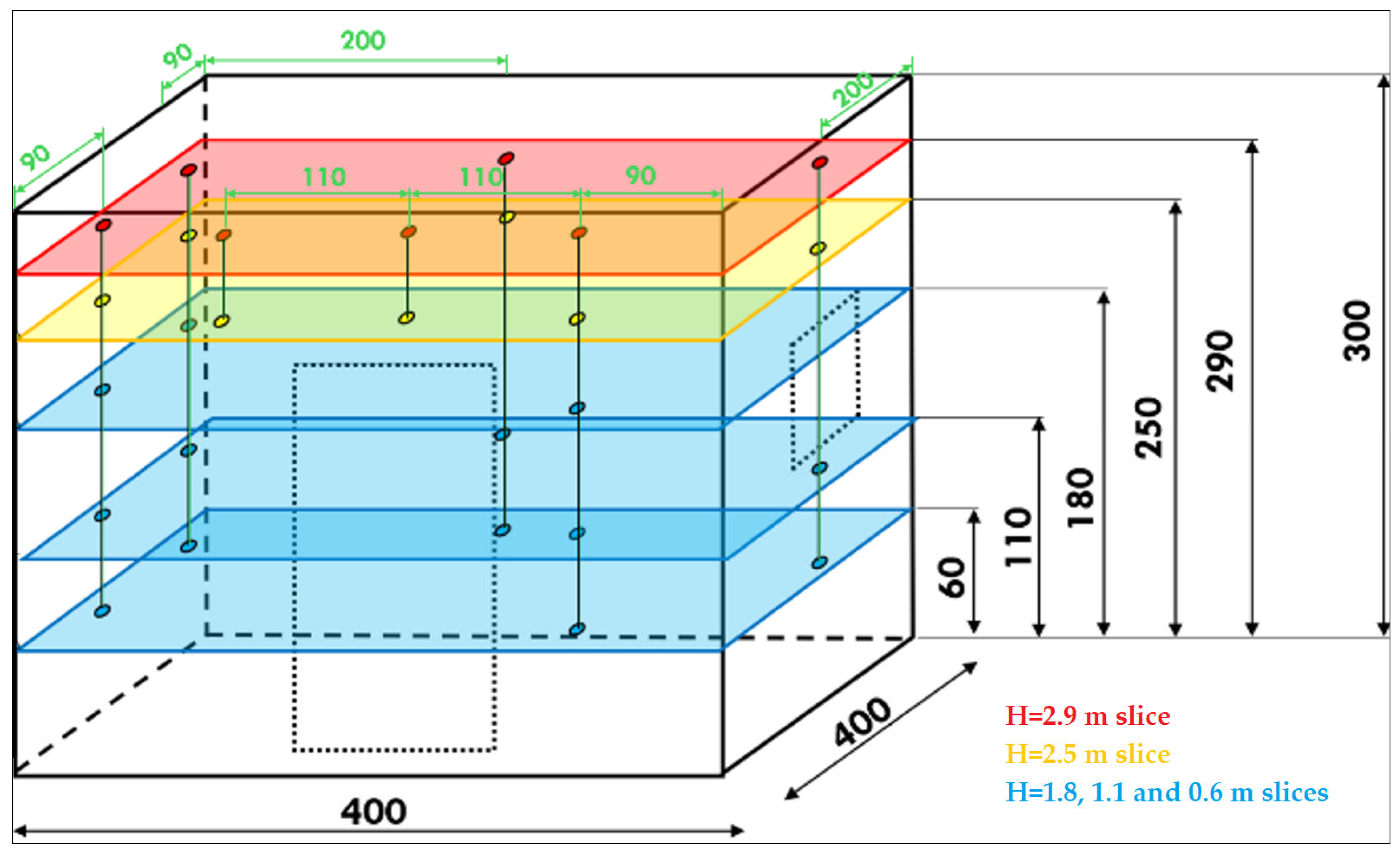
2.3. Experimental Equipment and Data Collection

The equipment used for temperature measurement consisted of 27 type K thermocouples embedded in the walls, featuring a refractory steel sheath with a diameter of 6 mm. These thermocouples are mass-isolated, flexible, equipped with G-type mounting nipples and a thread size of 3/8, “male-female” connectors, and cover a measurement range of 0 to 1200 °C, with a length of 400 mm. The thermocouples were grouped into 7 columns at 5 different heights, as shown in Figure 3, forming 5 temperature monitoring layers, each assigned one of three colors for easier result interpretation.
Additionally, 405 m of compensation cables were used for connecting the thermocouples, featuring silicone rubber insulation and sheath, with dimensions of 2 × 0.5 mm2, along with indicator controller devices that ensure temperature measurement and control, including selectable heating and cooling functions and adjustable temperature compensation, with an accuracy of ±0.25% full-scale or ±3 °C. The 5 planes were color-coded according to the height where they were mounted.
The values measured by the thermocouples were consolidated by the data acquisition module and subsequently processed for real-time access by the data collection station, both illustrated in Figure 4, which presents a detailed horizontal section of the experimental setup.

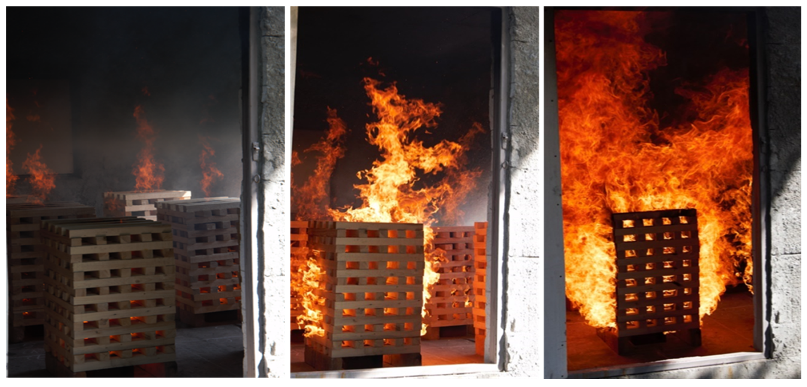
3. Experimental Results

The experiment took place at the Firefighters’ Faculty in May 2022 under normal atmospheric conditions, characterized by calm weather, no precipitation, and an ambient air temperature of 20 °C. The duration of the experiment was approximately 5 h, during which the maximum recorded temperature reached 836.4 °C, about 21 min after ignition. Figure 5 highlights the ignition stages of the wood cribs.
Figure 6 presents the temperatures measured by all thermocouples throughout the experiment. The monitored temperature evolution over time was segmented into four phases of the simulated fire development:
  • Slow burning phase (0–320 s);
  • Active burning phase (320–700 s);
  • Generalized burning phase (700–1280 s);
  • Regression phase (1280–1600 s).
The analysis of Figure 6 reveals significant variations in temperature values, with differences of up to 300 °C between levels, despite the reduced dimensions of the stand. While the upper levels showed minimal temperature fluctuations, the lower levels experienced pronounced variations during both the generalized burning phase and the regression phase.
Figure 7 highlights two critical moments in the experiment: the creation of conditions conducive to flashover occurrence and the extension of flames outside the stand.
Following the experiment, data collection, processing, and result interpretation, a numerical model was developed in PyroSim. This model aims to validate the numerical characteristics of the fire source, such as the value and temporal evolution of the HRR, the refinement of the computational domain (cell size), and the interior temperatures.

4. Development of the Numerical Model
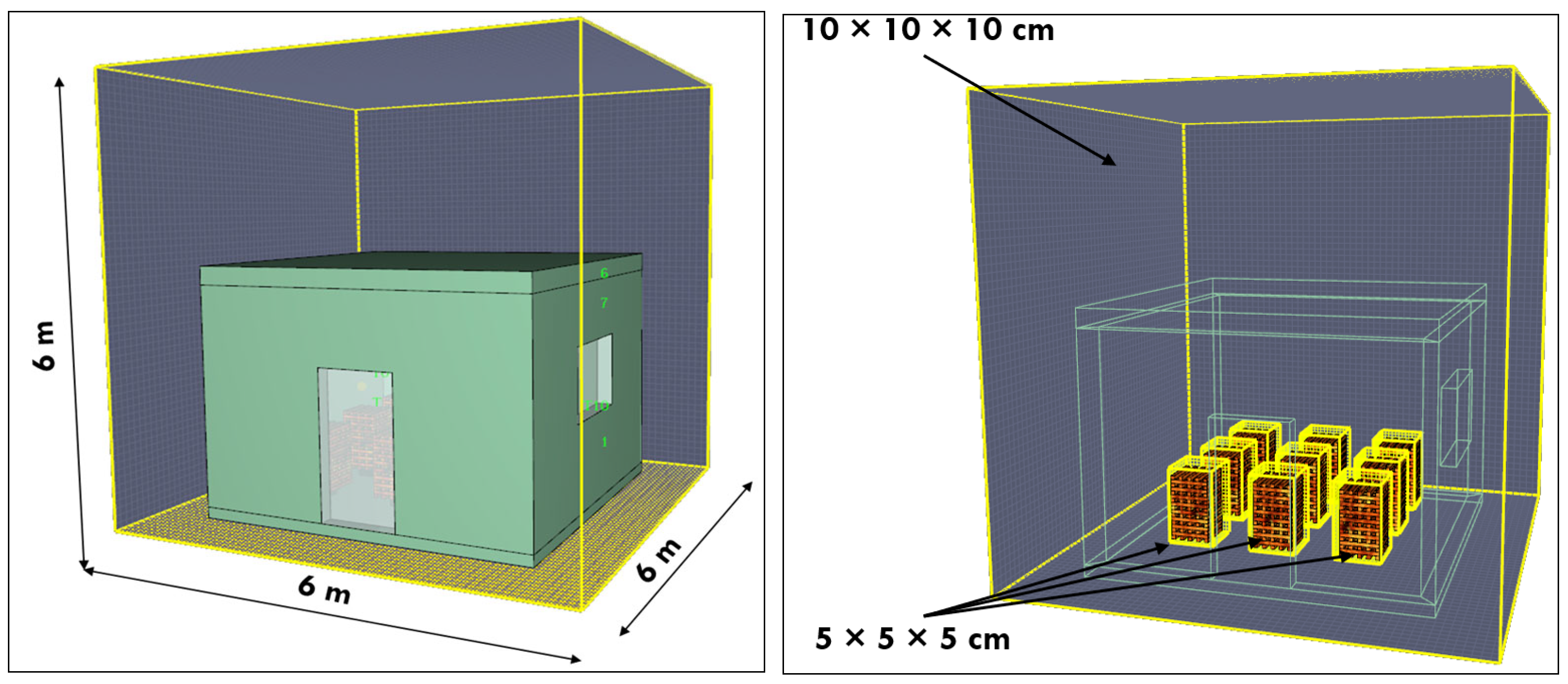
PyroSim, an inteface for FDS that employs CFD-based simulation methods, was selected as the simulation software due to its advanced capabilities in numerically modeling fire behavior and its recognized performance in experimental result calibration. The choice of this software is grounded in its ability to accurately simulate the complex phenomena of fires within a validated scientific framework, enabling precise correlation between experimental data and simulation outputs, thereby ensuring rigorous validation of the studied fire scenarios.

4.1. Model Geometry

The geometry of the experimental stand was constructed in accordance with the characteristics of the actual structure. Additionally, the geometry of the wood cribs was created in line with the previously described configuration. The model included two ventilation openings, specifically an open door and window, with further details illustrated in Figure 8.
Fire simulations were conducted using PyroSim 2023.3.1312, an interface that utilizes the FDS software version 6.7.9 [33,34,35]. The modeling of the phenomenon, carried out using this numerical simulation program, will be presented in the following section.

4.2. Domain and Mesh

For conducting simulations on the testing room, a simulation domain with dimensions exceeding those of the building was considered. This approach allows for the definition of varied climatic conditions and the observation of airflow phenomena both inside and outside the building. The domain was defined with dimensions of 6 × 6 × 6 m as shown in Figure 9.
The subdomains where the burner is located has dimensions of 0.6 × 0.6 × 1 m, situated at the lower part of the testing room on the ground floor, as shown in Figure 9.
In the calibration of the FDS model, extensive testing was conducted on various cell sizes—0.025 m, 0.05 m, 0.1 m, and 0.25 m—to determine the most effective mesh resolution and ensure a detailed reproduction of phenomena, similar to other studies [15,36,37]. This investigation revealed key insights, as the 0.25 m cell size was insufficiently refined to initiate a combustion reaction, yielding HRR values lower than those achieved with smaller cell sizes. Conversely, the 0.1 m cell size offered improved fidelity in heat transfer and smoke flow in regions adjacent to the fire source, yet it still fell short of matching experimental HRR values. The 0.5 m cell size demonstrated adequate precision for both adjacent domains and reaction initiation, though it required an eightfold increase in processing time and resources compared to the 0.1 m cell.
The evaluation of the 0.025 m cell size, despite providing a high accuracy of 1–2% relative to experimental data, was deemed impractical due to significantly higher resource and time costs—eight times that of the 0.05 m cell size. Consequently, a dual-mesh strategy was selected: utilizing a coarse 0.1 m cell for peripheral zones and a refined 0.05 m cell for the combustion focal area. This approach was calibrated to deliver results from a single simulation with an average relative error below 10%, efficiently completed in under 100 h. This analysis required eight trial simulations with reduced runtimes between 100 and 300 s.
An optimal mesh resolution necessitated compliance with the appropriate D∗/dx criterion, as identified in the literature, to ensure feasible results. We adhered to this framework, acknowledging that values ranging from 16.7 to 33.4 offer adequate precision. A D∗/dx value of 16.7 corresponds to a coarse mesh (0.1 m), while 33.4 represents a fine mesh (0.05 m), as shown in Figure 9.
Sensitivity analyses were conducted to evaluate the impact of mesh size on the convergence of heat flux and species concentration fields. While finer meshes improved field stability, they also increased computational demands [38,39,40]. In contrast, overly coarse meshes, as noted in [41], risk omitting critical details necessary for accurately capturing transient fire dynamics. Our investigation of mesh resolutions, using D∗/dx ratios between 16.7 and 33.4 [41,42,43], highlighted the influence of cell size on simulation accuracy, especially given the geometric complexity of the domain and the physical scale of the wooden cribs.
Mesh selection thus required balancing computational efficiency and predictive accuracy. Analysis of the Mean Relative Error (MRE), detailed in the calibration chapter, showed diminishing returns in accuracy when refining the mesh beyond a certain threshold—consistent with previous findings [41]. By adhering to validated D∗/dx values and performing systematic sensitivity testing, the FDS model was robustly calibrated, successfully replicating experimental conditions and reliably predicting fire behavior in open-plan office environments.
In conclusion, the number of cells in the burner subdomains was 25,920, while the cumulative number of cells of the domain left was 212,760. In total, the number of cells in the entire simulation domain was 238,680.

4.3. Boundary Conditions and Burner Characteristics

Regarding the domain boundary conditions, the lateral and upper surfaces were defined as “Open boundaries” using the simulation software’s predefined function, as detailed in the user manual [44]. This approach allows for natural air circulation within the domain, preventing constraints imposed by physical boundaries and eliminating the need to expand the domain size. At the time of the experiment, wind speed was negligible; thus, it was set to 0 m/s in the simulation, representing calm atmospheric conditions. The open boundaries method is widely recognized and used in CFD research, effectively and accurately simulating the upper air volume. This approach aligns with methodologies employed in other studies [45,46] and was validated by matching the environmental parameters to those of the real experiment. The simulation results demonstrated insensitivity to minor variations in these conditions, confirming the realism and robustness of the chosen settings.
In the entire simulation domain, the following environmental parameters were defined as follows:
-
Initial oxygen concentration was set to 20.8%;
-
Indoor temperature in the building was set to 20 °C;
-
Initial carbon dioxide concentration was set to 0.04%;
-
Initial visibility, at all points, was set to 30 m;
-
Atmospheric pressure was set to 101,325 Pa.
Inside the experimental stand, thermocouples were added at the same coordinates as shown in Figure 3 and Figure 4. In addition to temperature, the HRR value of the entire fire source was monitored. Numerical values of temperatures and HRR will be compared with experimentally obtained data for the purpose of calibrating the numerical model.
The composition of the fire source, the maximum HRR value per unit area, and the simplified HRR evolution curve were derived using the same two methods specified in the references [27,47], providing detailed guidelines for these procedures [24].
The combustion reaction in FDS requires that the combustible material be represented by a predefined and widely recognized chemical model consisting of four elements, with proportions C 3.4, H 6.2, O 2.5, and N 0 [30]. This model is well-established in the literature and has been validated using the PyroSim software developer’s calculator [42]. It focuses on simulating a single material and is known for accurately replicating real combustion reactions, particularly for wood, ensuring precise and feasible results while enhancing computational efficiency. This approach has been supported by various references [48,49,50,51,52].

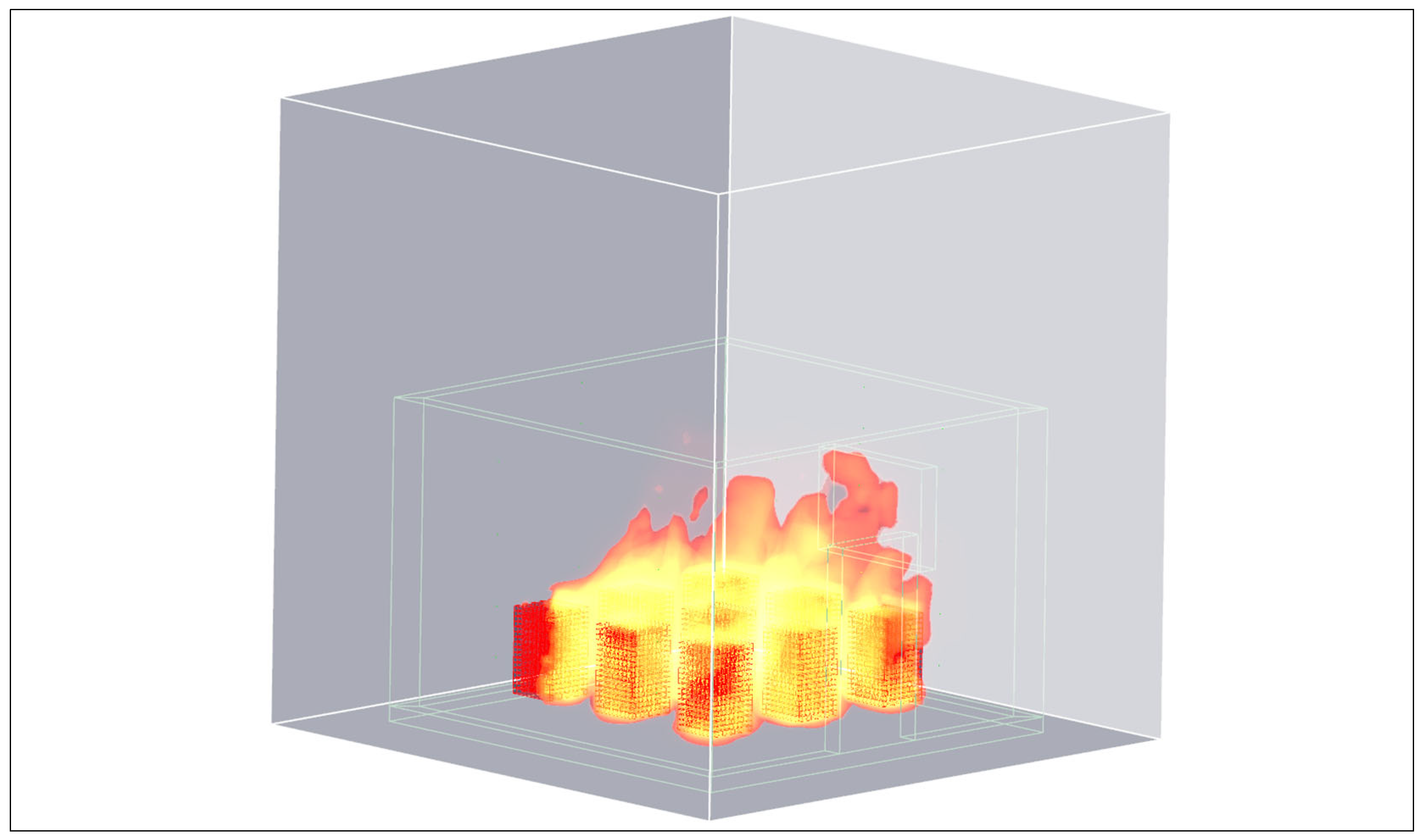
5. Numerical Results

The computation processing time for the 1280 s simulation was approximately 5 h, with the model being run on a workstation equipped with an Intel Core i9-13900K processor, 36M Cache, up to 5.80 GHz, and 32 GB RAM, manufactured by DELL Romania and purchased in Bucharest, Romania. The results obtained from the simulation will be presented next, collected through monitoring points and planes for temperature, velocity, and visibility. The monitoring points are located as indicated in Figure 3 and Figure 4 and gather data on temperature, speed, and concentrations of CO and CO2 in the air. The monitoring planes were positioned longitudinally and transversely, symmetrically sectioning the test space, as well as horizontally at heights of 1, 1.75, and 2.9 m.
Figure 10 highlights the dynamics of the simulated phenomenon and its impact on space. It captures intense burning with flames reaching window level, generating high temperatures and substantial smoke emission. The interdependence between fire and ventilation dictates the speed of propagation and direction of smoke, thereby affecting visibility and the safety of individuals.

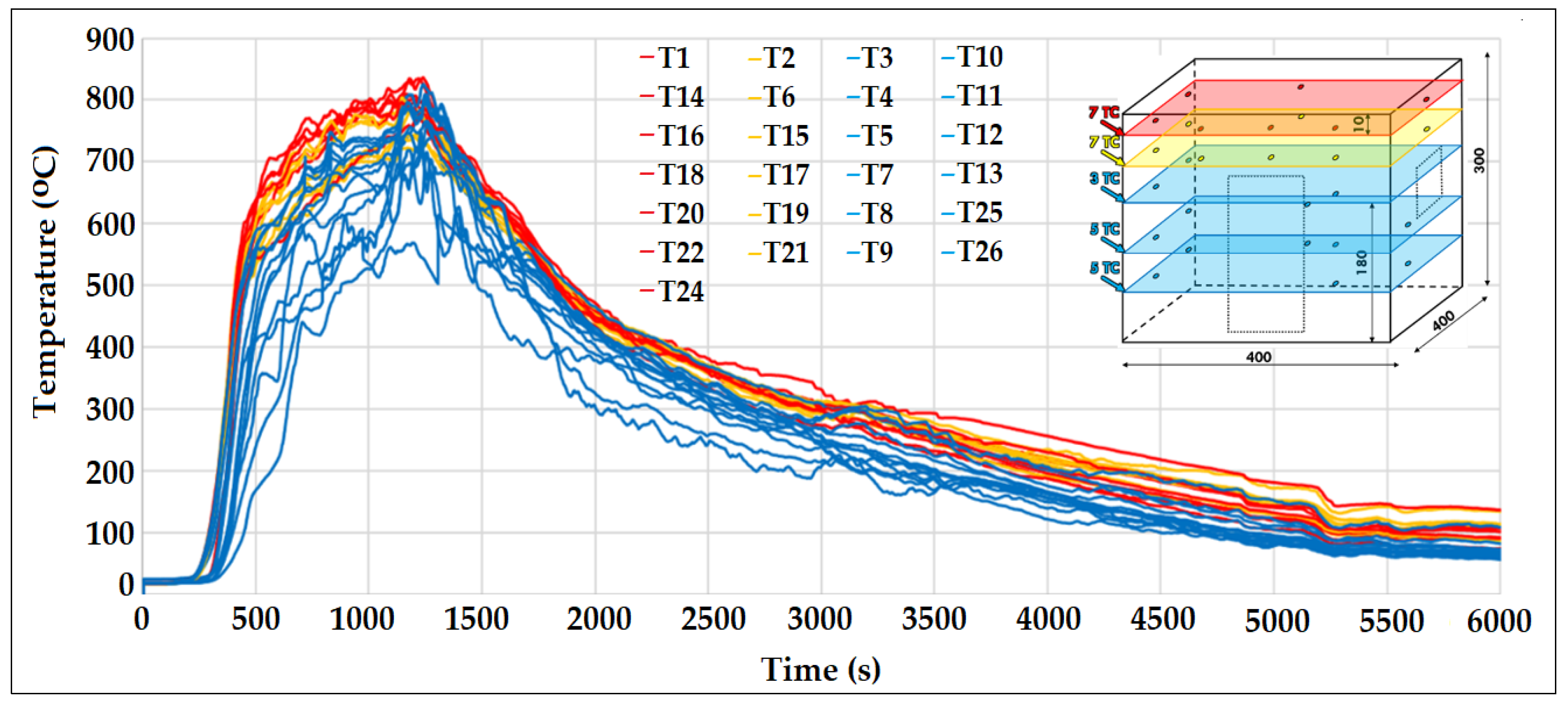
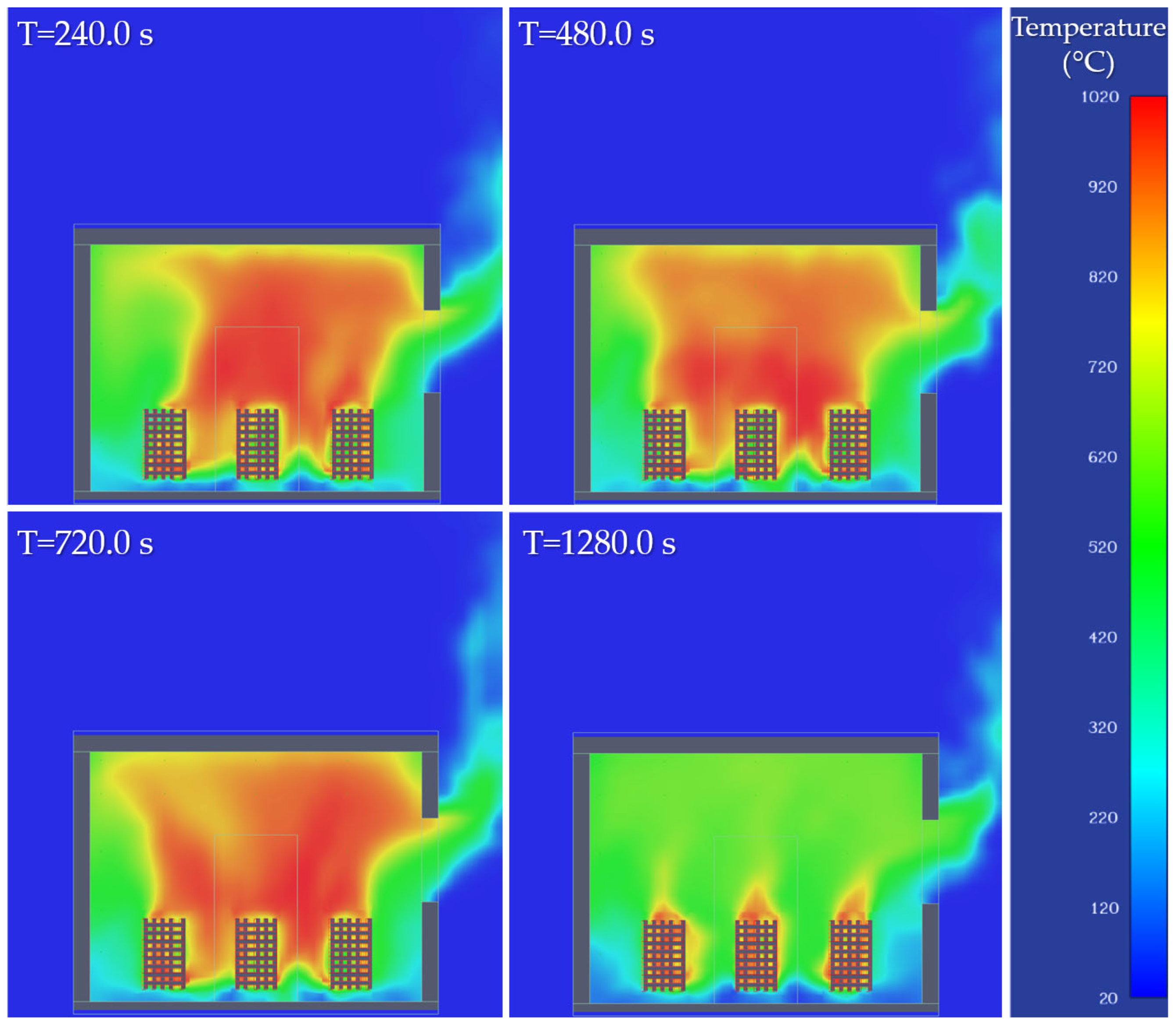
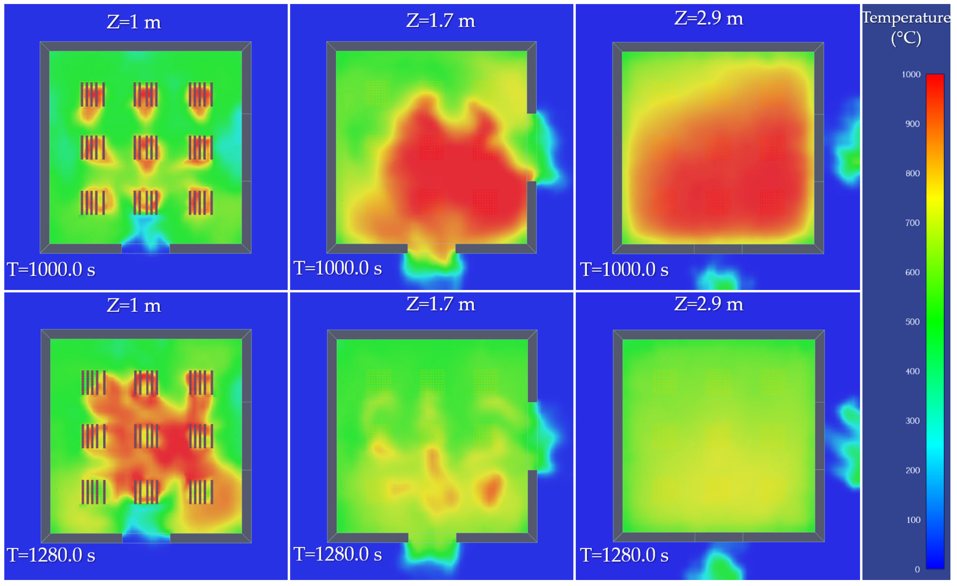
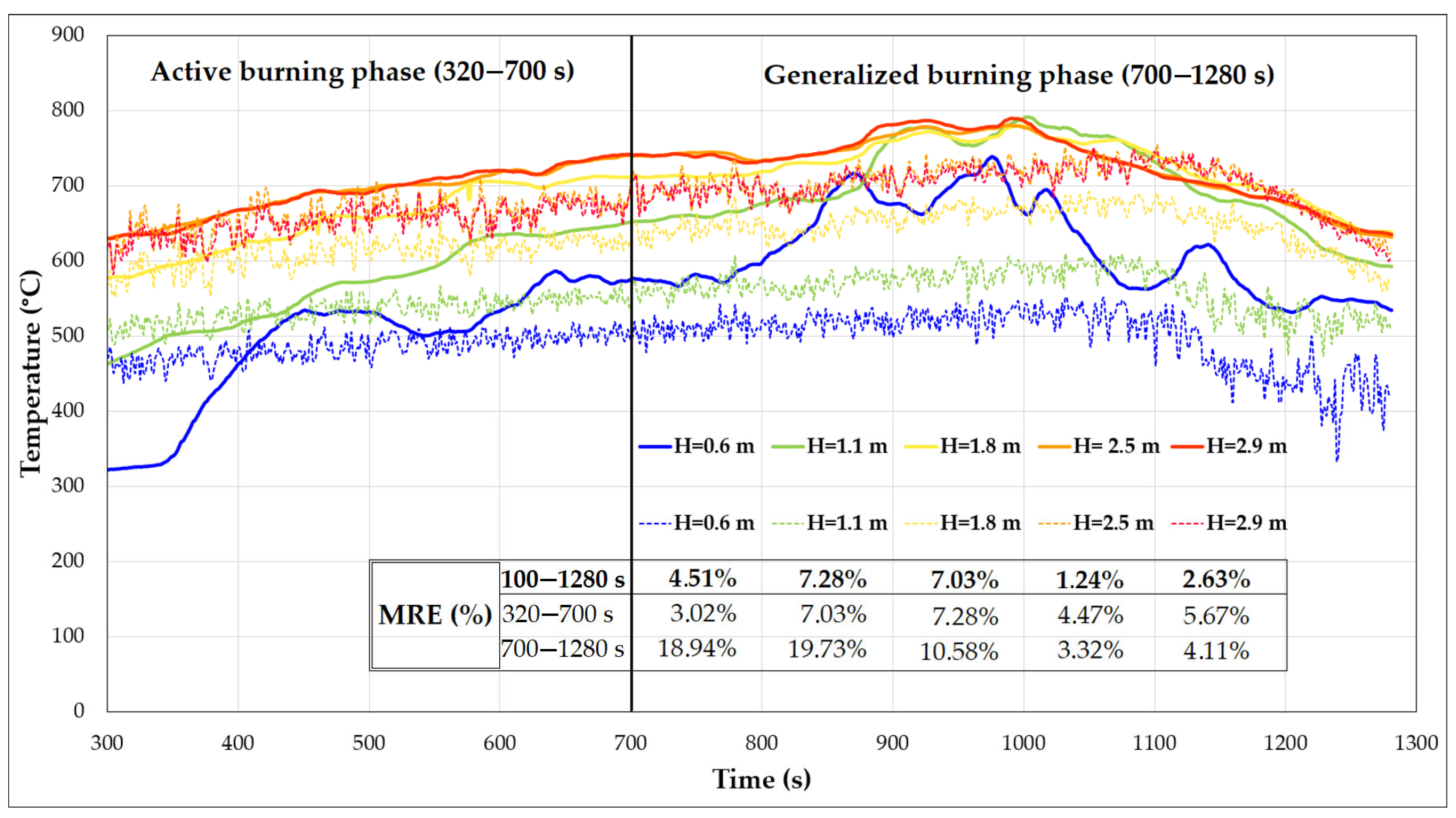
5.1. Temperature Variation Inside the Stand

Figure 11 illustrates the vertical distributions of temperature at different time intervals: 240, 480, 720, and 1280 s. Inside the stand, the temperature reached a peak value of 1020 °C at the fire source. At 240 s, the fire is well-developed, with the formation of an upper layer of hot gases reaching temperatures over 900 °C, highlighting a clear thermal stratification.
At 480 s, the compartment is almost completely filled with hot gases, and the outflow currents through the lateral opening are clearly defined, indicating stable ventilated burning. After 720 s, the temperature remains elevated, and the extension of the hot layer towards the floor confirms the continuation of the full burning phase. By 1280 s, a significant temperature drop is observed, signaling the onset of the stagnation phase of the fire as the oxygen concentration decreases due to the entire space being filled with smoke. The simulated behavior is representative of a fire in a ventilated space with controlled burning.
Figure 12 illustrates the evolution of horizontal temperature distribution at three height levels (Z = 1 m, 1.7 m, and 2.9 m) within the compartment at times T = 1000 s and T = 1280 s. A pronounced stratification of hot gases is observed, a phenomenon characteristic of the full burning phase, particularly evident at Z = 2.9 m, where the entire room area is dominated by high temperatures (over 700–800 °C) at T = 1000 s. At the mid-level (Z = 1.7 m), the temperature is also high, but with a more uneven distribution, indicating partial accumulation of combustion gases. At the lower level (Z = 1 m), active burning around the wood cribs is well-defined, with an influx of cold air through the opening situated at the bottom of the exterior wall.
At T = 1280 s, the temperature distribution visibly decreases at all levels, indicating a clear transition to a stagnation phase of the fire. The hot gases in the upper layer have dissipated significantly, and the intensity of the active fire at the crib level has diminished, confirming a progressive inhibition of the combustion reaction due to low oxygen concentration. These horizontal views coherently highlight the vertical temperature dynamics during the fire, being relevant for assessing the ventilation efficiency, thermal stratification, and the potential thermal hazard in different areas of the compartment.

5.2. Air Velocity Variation Inside the Stand

Figure 13 illustrates the horizontal distribution of gas velocity at three height levels (Z = 1 m, 1.7 m, and 2.9 m) at times T = 1000 s and T = 1280 s. At T = 1000 s, during the generalized burning phase, there is intense activity around the fire source (Z = 1 m), where velocities exceed 3 m/s, indicating strong convective movements due to massive thermal energy release. At the upper level (Z = 2.9 m), the flow of hot gases is predominantly evacuated through the upper opening, reaching local velocity values over 5 m/s, which suggests good natural ventilation. In the mid plane (Z = 1.7 m), the flows are more diffused and with lower velocities, indicating a relatively stagnant area between ascending and evacuated currents. At T = 1280 s, with the reduction in burning intensity, the velocity distribution significantly decreases across all levels.
Values remain moderate only near the ventilation points, confirming the transition to a decay phase of the fire, where gas movements are driven more by residual thermal inertia than by active combustion. These visualizations contribute to the understanding of the aerodynamic behavior of combustion gases and are crucial for fire safety analysis and the sizing of smoke evacuation systems.

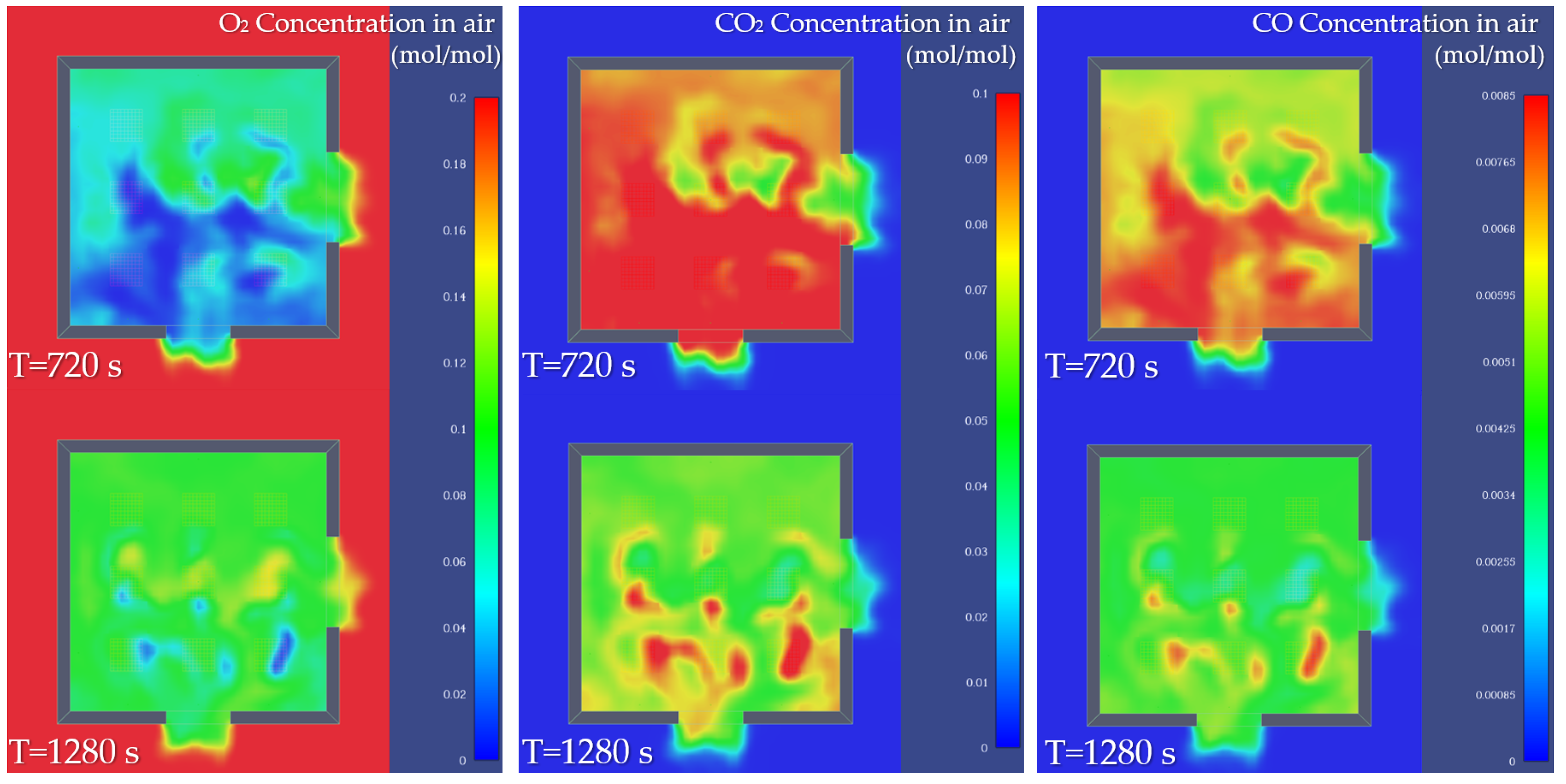
5.3. Visibility and CO/CO2 Concentration Variation Inside the Stand

Visibility within a fire-affected space is determined by the concentration and opacity of smoke particles that absorb and scatter light. In the early stages of a fire, visibility is quickly reduced due to the accumulation of fine particles. Visibility is closely correlated with concentrations of carbon monoxide and dioxide, as high levels of these toxic gases inherently lead to very low visibility and thus hostile evacuation conditions for occupants.
Figure 14 shows the distributions of oxygen (O2), carbon dioxide (CO2), and carbon monoxide (CO) concentrations within the simulated fire in the stand at times 720 and 1280 s. At T = 720 s, observations indicate a reduced O2 concentration, below 12%, corresponding to the onset of an incomplete burning stage, where oxygen remains sufficient to support combustion reactions. This consumption of O2 is reflected in elevated levels of CO2 and CO, indicating a combustion cycle in which the incomplete burning of wood generates measurable levels of toxic gases.
Considering the ventilated burning regime, well-defined evacuation flows reveal that hot gases are systematically discharged, initially favoring the maintenance of fuel combustion. However, at T = 1280 s, a partial recovery of O2 concentration and a decrease in temperature are observed, correlated with reduced CO2 and CO concentrations in the simulated space. This indicates that the fire is entering a stagnation/regression phase, driven by both the depletion of the fuel source and the oxygen necessary for sustained combustion.
When comparing gas concentrations with the thermal distribution, a combustion dynamic influenced by the availability of oxygen is observed, where its reduction plays a crucial role in decreasing the intensity of the simulated fire.

6. Numerical Model Calibration

6.1. Calibration Methodology

The calibration of the numerical model against the experimentally obtained data was primarily based on HRR, with temperature serving as a secondary reference. Despite its secondary role, temperature still provided essential insights into vertical gradients during key phases like flashover. This dual process is also aimed at validating the accuracy of the numerical model. To optimize the process of obtaining numerical data, a refinement analysis of the domain was conducted in the current phase to produce feasible results with minimal resource consumption. As a result, three known and independent input parameters were varied (as shown in Table 1), generating a total of eight simulations. Recognizing that the full experimental duration was approximately 16,000 s (5 h), the simulation was limited to 1280 s to capture the key phases of fire evolution effectively.
To assess the accuracy of the simulations, two quantitative indicators were used: Mean Relative Error (MRE) and Root Mean Square Error (RMSE) over a relevant time interval, hereafter referred to as the “useful interval”. The useful interval was defined as the period during which both experimental data and numerical results are relevant and comparable, capturing the key fire phases while maintaining computational efficiency. Its definition was necessary because the aim was not to conduct a time-intensive simulation equivalent in duration to the experiment. Given that the maximum temperature was recorded at T = 1234 s, it was deemed appropriate to limit the simulation duration to 1280 s. This allowed for the inclusion of all defining phases of fire evolution while ensuring a reasonable computation time for the simulations. The useful interval was established after excluding an initial period, spanning from T = 100 s to T = 1280 s, and was determined to be ample for optimal model calibration.
For MRE, comparison will adhere to an acceptability threshold of ±10% within the useful interval, with values outside this range being deemed unsatisfactory for validation purposes. For RMSE, a systematic approach was employed by constructing an error matrix (Figure 15) that combines three independent sets of factors, each with two variants (2 × 2 × 2): cell size, source intensity (HRRPUA), and type of domain discretization. Each combination will result in an RMSE value calculated over the same useful interval, with the configuration yielding the lowest error being considered the most precise and relevant model in terms of proximity to experimental reality. The objective in evaluating the numerical model’s accuracy was to achieve an optimal balance between result precision, with RMSE minimized, MRE falling within a ±10% margin, and computation time not exceeding 100 h (Table 1).

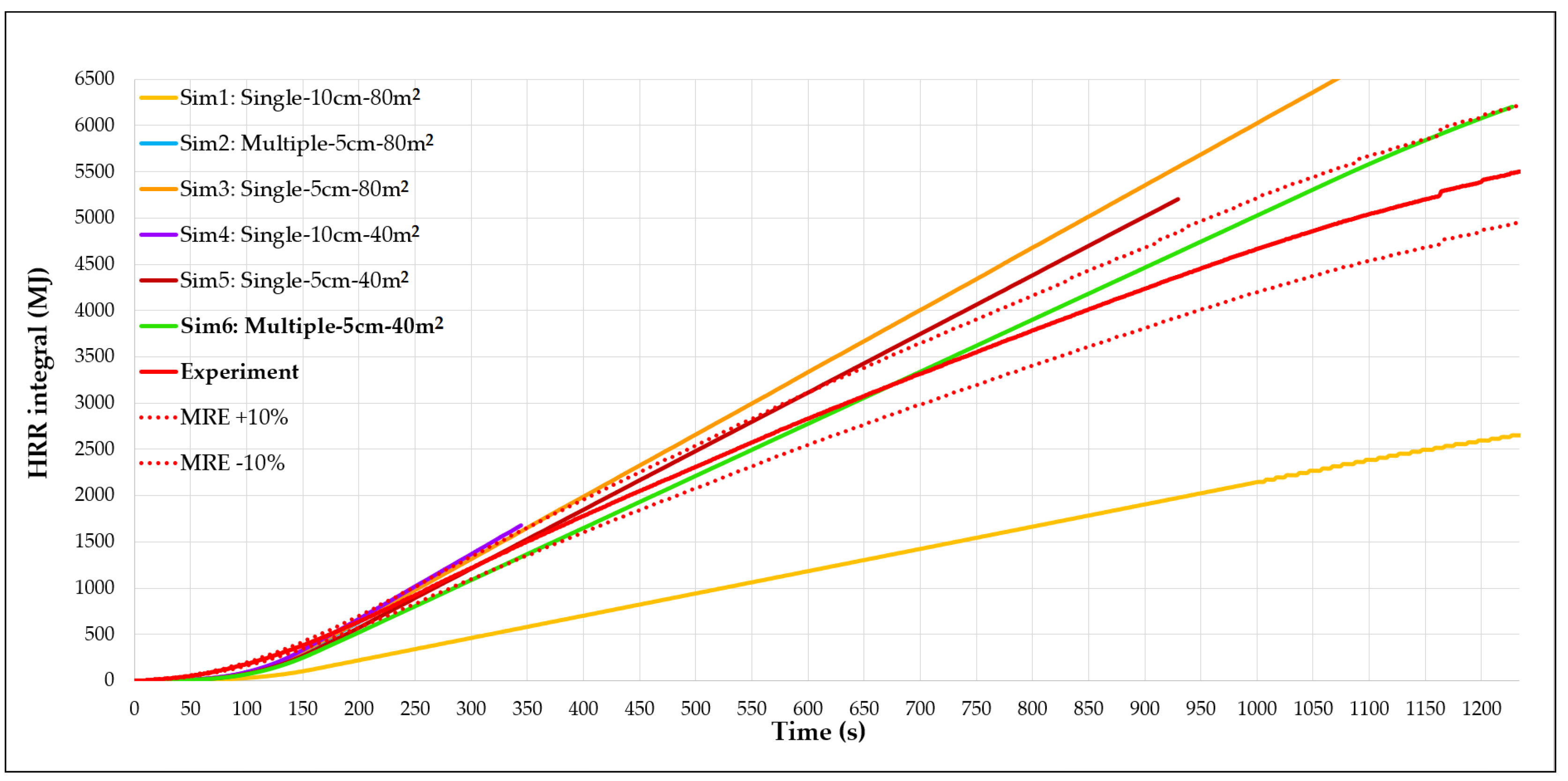
6.2. Calibration Based on HRR

The accuracy of the numerical model calculated using MRE was performed for all 8 simulations. Among these simulations, only 6 produced results comparable to the experimental data or were completed within a reasonable processing time. Of the tested variants, the simulation labeled “Sim 6” (marked in green in Figure 16), which employs a cell size of 5 cm, a cumulative fire source area of 40.16 m2, and an individualized domain subdivision as shown in Figure 9, offered the best compromise between result accuracy and computation time. As illustrated in Figure 16, the curve corresponding to Sim 6 closely follows the entire experimental HRR evolution, with no significant differences observed throughout the analyzed interval.
The accuracy of the model calculated using MRE over the entire 1280 s interval was 10.12%, which is considered within the acceptable error range. However, over the useful interval of 100 to 1234 s, representing approximately 92% of the simulation duration, the accuracy calculated with MRE was only 5.04%. The active phase is reproduced with very high accuracy (error 2.9%), while in the generalized phase, deviations increase slightly (6.5%), mainly due to cumulative uncertainties in fuel surface regression and ventilation dynamics. This suggests that significant discrepancies occur in the initial moments of the simulation, attributed to the slightly inaccurate prediction of the dead time.
The discrepancies in HRR between the numerical model and the experiment are primarily attributed to several factors, with cell size being a significant contributor. Additionally, the use of a standard calorific power value of 17.5 MJ/kg for wood, based on the current regulations [11], introduced variability, as it was not feasible to measure this value for each wooden bar individually. Differences in wood properties, likely due to varying tree sources, further contributed to inconsistencies. These factors were recognized and incorporated within the acceptable margin of error to ensure the reliability of the HRR calibration.

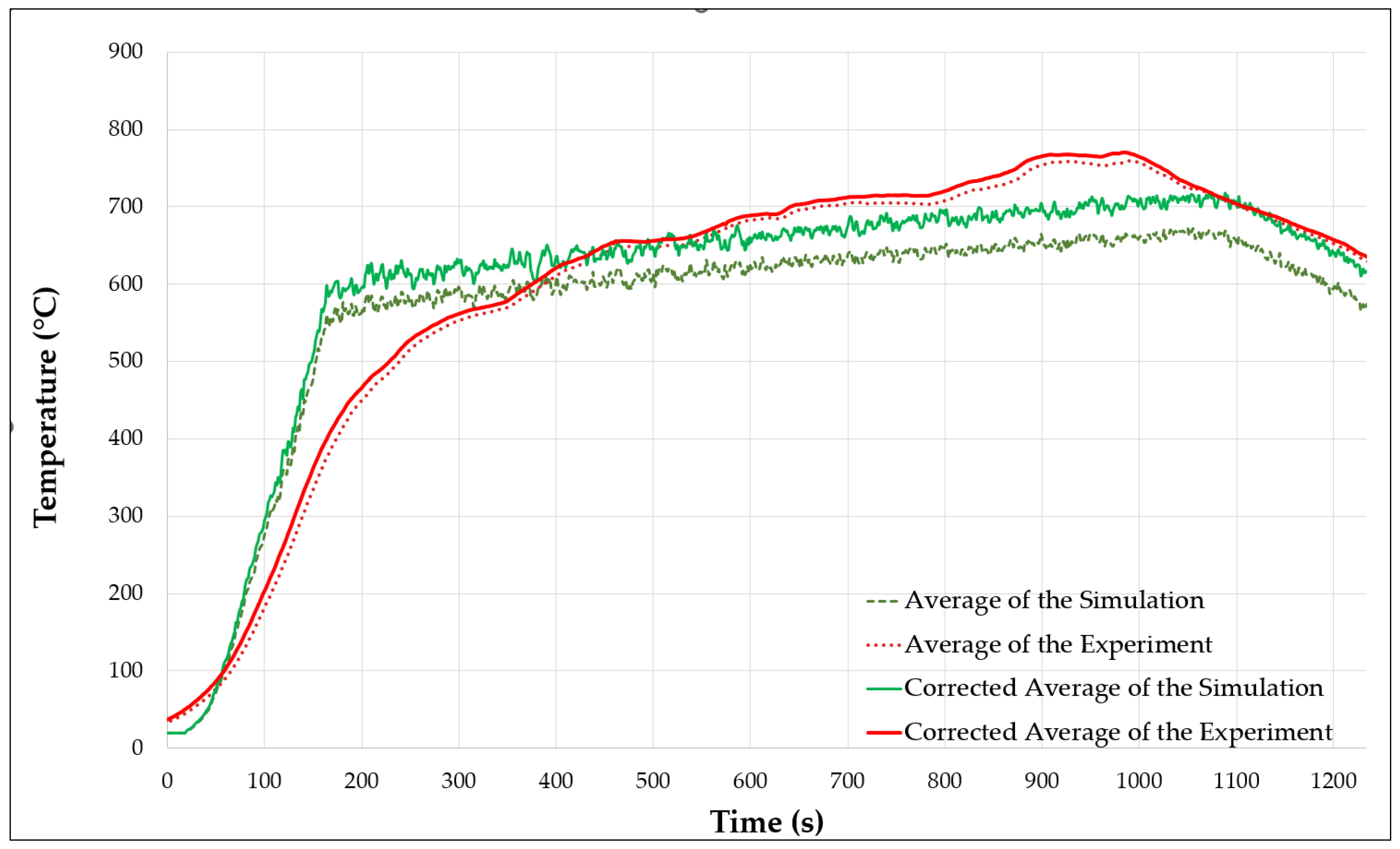
6.3. Calibration Based on Temperature

To calibrate the numerical model according to temperature values obtained both experimentally and numerically, the average values from all 27 thermocouples were used throughout the simulation. These average values are presented in Figure 17 (black dashed lines). It is observed that the trends are similar and the general tendency is maintained. The mean error between the two graphs was also calculated, resulting in approximately 17.79%. This value, considering the number of thermocouples, the size of the stand, the duration of the experiment, and the thermal load, is deemed acceptable.
The analysis of individual mean errors, shown in Table 2, reveals that out of the 27 thermocouples used, 17 recorded a mean error below 10%, 5 had values between 10% and the overall mean error value (17.79%), and 5 exceeded this threshold. These results indicate a satisfactory agreement between simulated and experimental values for the majority of measurement points, with errors under 3% in some cases. Only a limited number of thermocouples exhibited significant deviations, with errors exceeding 20%.
Excluding from the analysis the four thermocouples that exhibited errors over 40% (outliers) would substantially reduce the corrected mean error from 17.79% to 6.9%. This revised mean error value further confirms that the prediction of data obtained from the simulation is acceptable and supports the conclusion drawn from HRR analysis regarding the validity of the numerical model. The corrected averages of the temperatures monitored during the experiment (solid red line) and the simulation (solid green line) are presented in Figure 17.
The substantial reduction in the mean error underscores the importance of addressing outliers to enhance the alignment between experimental and simulated data. This refinement not only validates the numerical model but also strengthens confidence in its predictive capabilities for future fire behavior simulations under similar conditions.
To capture the vertical temperature profile in a consistent and protected location, we instrumented two vertical thermocouple trees, each consisting of five sensors placed at heights of 0.6 m, 1.1 m, 1.8 m, 2.5 m, and 2.9 m, on the left wall (X = 0.10 m) of the enclosure. This wall was selected because it had no openings, ensuring uniform exposure to the developing hot gas layer. In contrast, the other walls either had too few sensors or featured non-uniform placements, which made them less suitable for extracting reliable vertical gradients.
The results presented in Figure 18 clearly illustrate the expected vertical stratification of temperature, with values increasing consistently with height. This gradient is especially evident in the generalized burning phase, where the upper thermocouples register significantly higher temperatures compared to the lower ones. The numerical model reproduces this stratification well, particularly in the upper layers (2.5 m and 2.9 m), where thermal conditions are more stable and dominated by buoyancy-driven flow.
To evaluate the model’s predictive accuracy, we focused on two key fire stages: the active burning phase (320–700 s) and the generalized burning phase (700–1280 s). As shown in Figure 18, the model closely matches the experimental data during the active phase, capturing both the vertical temperature increase and maintaining low Mean Relative Errors across all sensor heights.
In the generalized burning phase, discrepancies become more evident, particularly at lower heights (0.6 m and 1.1 m), where the model tends to underestimate temperatures—likely due to complex mixing and descending cooler air near the floor. However, in the upper layers (2.5 m and 2.9 m), the model continues to show good agreement with measured values, reflecting a reliable prediction of the hot gas layer behavior.
Overall, the stratification profiles in Figure 18 confirm that the model accurately captures the vertical temperature gradient, especially during the active phase and in the upper part of the enclosure. Despite some underestimations near the floor during the generalized phase, the results remain within acceptable accuracy margins, supporting the model’s use for simulating vertical thermal dynamics in compartment fires.
Temperature discrepancies arose primarily from four thermocouples that displayed errors over 40%, as these were positioned near the door where local turbulent eddies and sustained smoke flow were prevalent throughout the experiment. Although FDS, with its Very Large Eddy Simulation (VLES) capabilities, models fluid flows accurately, it can occasionally miss capturing such turbulence, leading to discrepancies. However, with a greater number of thermocouples, these negative effects can be mitigated. By excluding these outliers, the mean error was reduced from 17.79% to 6.9%. In the post-experiment analysis, it was observed that employing 96–120 thermocouples would provide a more comprehensive capture of thermal gradients, thus enhancing the overall predictive accuracy of the simulation model.

7. Conclusions

The experiment conducted within the stand achieved its objectives, successfully replicating the effects of an office fire and contributing to the calibration of the presented numerical model based on two parameters, HRR and temperature. Due to the very high temperatures and smoke emissions, such a fire, if triggered in an office building, would involve a large number of occupants needing to evacuate quickly through a limited number of escape routes. Additionally, due to the dynamic nature of fire evolution and the development of thermal draft within the building during occupant evacuation, combustion products from burning plastic materials can lead to carbon monoxide and dioxide poisoning, which is the primary cause of death in fires.
In the full-scale experiment, temperatures of a simulated fire with a substantial thermal load of 6720 MJ were determined. As observed, the simulated fire progressed violently, frequently reaching temperatures above 800 °C. A normal ventilation scenario was chosen, involving keeping the stand’s door and window open. The quality of the wood burned significantly influenced the research results, with the thermal load depending on the wood’s moisture content. A higher moisture content in the wood would have significantly reduced the thermal load.
The experimental results obtained were correlated with data from numerical simulations conducted on the same stand, focusing on calibrating and validating the numerical model of the experimental stand. In the numerical study, the HRR value and the optimal subdomain cell size were validated to ensure the results obtained were as feasible and relevant as possible. The study aimed for high efficiency since, in the subsequent phase, a large number of simulations (10–15) and a potential extension of the numerical model from the room level (office) to the building level were desired. Therefore, low efficiency could have irreversibly influenced the simulation processing time and potentially compromised the successful completion of this research program.

Author Contributions

I.-C.E., main author, significantly contributed to the initial drafting of the manuscript, the study’s methodology, software utilization, data validation, interpretation of results and raw data, as well as formal analysis and project administration. V.I., main author, was responsible for the conceptualization of the research, interpretation of data and results, manuscript review, supervision and project administration. M.D., the third author, was responsible for procuring materials and constructing the stand, ensuring comprehensive supervision throughout the process. I.A., the fourth author, provided optimal project management and secured the funding source necessary to guarantee the computational power required for the numerical model. All authors have read and agreed to the published version of the manuscript.

Funding

This research work would not have been possible without the use of workstations from the “CFD Fire Simulation and Evacuation for Large Infrastructures” Laboratory, developed through the project “Development of an Innovative Center for Smart Digital Coordination”, funded by the National Recovery and Resilience Plan, Component C15: Education/Reform 5: Adoption of the Legislative Framework for the Digitalization of Education/Investment 16: Digitalization of Universities and Their Preparation for the Digital Professions of the Future”. The digitalization project “Development of an Innovative Center for Smart Digital Coordination”, project code e-PNRR: 2031753094, was approved by the Order of the Minister of Education No. 4168/30.06.2022. The Funding Contract No. 14017 dated 16.09.2022 is between the “Alexandru Ioan Cuza” Police Academy and the Ministry of Education.

Institutional Review Board Statement

Not applicable.

Informed Consent Statement

Not applicable.

Data Availability Statement

The original contributions presented in the study are included in the article. Further inquiries can be directed to the corresponding authors.

Acknowledgments

We wish to extend our gratitude to Florin Bode for his valuable expertise, careful guidance, and constant support in the development of this work.

Conflicts of Interest

The authors declare no conflicts of interest.

References

  1. McMahon, C. OSHA Office Space Requirements Per Person in 2023. Zippia. 2023. Available online: https://www.zippia.com/advice/how-much-office-space-per-employee/ (accessed on 14 May 2025).
  2. CBRE. Market Outlook H1 2023, Romania Real Estate Report. 2023. Available online: https://mktgdocs.cbre.com/2299/e8e123c5-f516-46db-a17e-bcf28937f65e-799713409.pdf (accessed on 14 May 2025).
  3. Alarie, Y. Toxicity of Fire Smoke. Crit. Rev. Toxicol. 2002, 32, 259–289. [Google Scholar] [CrossRef] [PubMed]
  4. Mei, F.; Tang, F.; Ling, X.; Yu, J. Evolution characteristics of fire smoke layer thickness in a mechanical ventilation tunnel with multiple point extraction. Appl. Therm. Eng. 2017, 111, 248–256. [Google Scholar] [CrossRef]
  5. La Nasa, J.; Lomonaco, T.; Manco, E.; Ceccarini, A.; Fuoco, R.; Corti, A.; Modugno, F.; Castelvetro, V.; Degano, I. Plastic breeze: Volatile organic compounds (VOCs) emitted by degrading macro- and microplastics analyzed by selected ion flow-tube mass spectrometry. Chemosphere 2021, 270, 128612. [Google Scholar] [CrossRef]
  6. Woolley, W.D.; Raftery, M.M. Smoke and toxicity hazards of plastics in fires. J. Hazard. Mater. 1975, 1, 215–222. [Google Scholar] [CrossRef]
  7. Gormsen, H.; Jeppesen, N.; Lund, A. The causes of death in fire victims. Forensic Sci. Int. 1984, 24, 107–111. [Google Scholar] [CrossRef]
  8. Ene, I.-C.; Iordache, V.; Becheru, A.-G. The influence of ventilation factors on the development of fires in rooms and buildings. Review of numerical studies. Rom. J. Civ. Eng. 2023, 14, 96–106. [Google Scholar] [CrossRef]
  9. Babrauskas, V.; Williamson, R. The historical basis of fire resistance testing—Part I. Fire Technol. 1978, 14, 184–194. [Google Scholar] [CrossRef]
  10. Ariyanayagam, A.D.; Mahendran, M. Fire Safety of Buildings Based on Realistic Fire Time-Temperature Curves. In Proceedings of the 19th International CIB World Building Congress, Brisbane 2013: Construction and Society, Brisbane, Australia, 5–9 May 2013. [Google Scholar]
  11. EN 1991-1-2: 2005; Eurocode 1: Actions on Structures—Part 1-2: General Actions—Actions on Structures Exposed to Fire. European Committee for Standardization (CEN): Brussels, Belgium, 2005.
  12. Van Mierlo, R.; Sette, B. The Single Burning Item (SBI) test method-a decade of development and plans for the near future. Heron 2005, 50, 191–208. [Google Scholar]
  13. Proulx, G. Highrise evacuation: A questionable concept. In Proceedings of the 2nd International Symposium on Human Behaviour in Fire, London, UK, 12–14 March 2001; pp. 221–230. [Google Scholar]
  14. ISO 13943:2017; Fire Safety-Vocabulary. International Organization for Standardization: Geneva, Switzerland, 2017.
  15. Brohez, S.; Caravita, I. Fire induced pressure in airthigh houses: Experiments and FDS validation. Fire Saf. J. 2020, 114, 103008. [Google Scholar] [CrossRef]
  16. Gao, R.; Fang, Z.; Li, A.; Shi, C.; Che, L. Estimation of building ventilation on the heat release rate of fire in a room. Appl. Therm. Eng. 2017, 121, 1111–1116. [Google Scholar] [CrossRef]
  17. Yuan, M.; Chen, B.; Li, C.; Zhang, J.; Lu, S. Analysis of the Combustion Efficiencies and Heat Release Rates of Pool Fires in Ceiling Vented Compartments. Procedia Eng. 2013, 62, 275–282. [Google Scholar] [CrossRef]
  18. Himoto, K.; Shinohara, M.; Sekizawa, A.; Takanashi, K.; Saiki, H. A field experiment on fire spread within a group of model houses. Fire Saf. J. 2018, 96, 105–114. [Google Scholar] [CrossRef]
  19. Shi, W.; Ji, J.; Sun, J.; Lo, S.; Li, L.; Yuan, X. Experimental Study on the Characteristics of Temperature Field of Fire Room under Stack Effect in a Scaled High-rise Building Model. Fire Saf. Sci. 2014, 11, 419–431. [Google Scholar] [CrossRef]
  20. Miloua, H.; Azzi, A.; Wang, H.Y. Evaluation of different numerical approaches for a ventilated tunnel fire. J. Fire Sci. 2011, 29, 403–429. [Google Scholar] [CrossRef]
  21. Leisted, R.R.; Sørensen, M.X.; Jomaas, G. Experimental study on the influence of different thermal insulation materials on the fire dynamics in a reduced-scale enclosure. Fire Saf. J. 2017, 93, 114–125. [Google Scholar] [CrossRef]
  22. Stewart, J.R.; Phylaktou, H.N.; Andrews, G.E.; Burns, A.D. Evaluation of CFD simulations of transient pool fire burning rates. J. Loss Prev. Process Ind. 2021, 71, 104495. [Google Scholar] [CrossRef]
  23. Bolina, F.L.; Fachinelli, E.G.; Pachla, E.C.; Centeno, F.R. A critical analysis of the influence of architecture on the temperature field of RC structures subjected to fire using CFD and FEA models. Appl. Therm. Eng. 2024, 247, 123086. [Google Scholar] [CrossRef]
  24. Ene, I.-C.; Iordache, V.; Anghel, I. The Impact of an Office Fire Combined with the Stack Effect in a Multi-Story Building. Appl. Sci. 2024, 14, 11659. [Google Scholar] [CrossRef]
  25. Harvie, D.J.E.; Novozhilov, V.; Kent, J.H.; Fletcher, F.D. An experimental study of wood crib extinguishment by a sprinkler spray. J. Appl. Fire Sci. 1999, 8, 247–263. [Google Scholar] [CrossRef]
  26. Larsson, I.; Ingason, H.; Arvidson, M. Model Scale Fire Tests on a Vehicle Deck on Board a Ship. 2005. Available online: http://www.diva-portal.org/smash/get/diva2:962221/FULLTEXT01.pdf (accessed on 20 May 2025).
  27. Xu, Q.; Griffin, G.J.; Jiang, Y.; Bicknell, A.D.; Bradbury, G.P.; White, N. Calibration burning of wood crib under ISO9705 hood. J. Therm. Anal. Calorim. 2008, 91, 355–358. [Google Scholar] [CrossRef]
  28. ISO 9705-1:2016; Reaction to Fire Tests—Room Corner Test for Wall and Ceiling Lining Products—Part 1: Test Method for a Small Room Configuration. ISO: Geneva, Switzerland, 2016; p. 42.
  29. SR EN 1991-1-2:2004; Eurocode 1: Actions on Structures—Part 1-2: General Actions—Actions on Structures Exposed to Fire. Romanian Standards Association (ASRO): Bucharest, Romania, 2004.
  30. Degler, J.; Eliasson, A.; Anderson, J.; Lange, D.; Rush, D. A-Priori Modelling of the Tisova Fire Test as Input to the Experimental Work. In Proceedings of the 1rst International Conference on Structural Safety under Fire & Blast, Glasgow, UK, 2–4 September 2015. [Google Scholar]
  31. Dima, M. Research Report No. 3; Technical University of Civil Engineering of Bucharest: Bucharest, Romania, 2021. [Google Scholar]
  32. Karlsson, B.; Quintiere, J.G. Enclosure Fire Dynamics; CRC Press: Boca Raton, FL, USA, 1999. [Google Scholar]
  33. Glenn, P. Forney Smokeview, A Tool for Visualizing Fire Dynamics Simulation Data: User’s Guide; NIST Special Publication: Gaithersburg, MD, USA, 2016; Volume I, p. 223. Available online: https://pages.nist.gov/fds-smv/manuals.html (accessed on 18 May 2025).
  34. Glenn, P. Forney Smokeview, A Tool for Visualizing Fire Dynamics Simulation Data: Verification Guide; NIST Special Publication: Gaithersburg, MD, USA, 2016; Volume III, p. 105. Available online: https://www.nist.gov/publications/smokeview-version-6-tool-visualizing-fire-dynamics-simulation-data-volume-iii (accessed on 18 May 2025).
  35. Glenn, P. Forney Smokeview, A Tool for Visualizing Fire Dynamics Simulation Data: Technical Reference Guide, NIST Special Publication : Gaithersburg, MD, USA, 2016; Volume II, p. 88. Available online: https://www.fse-italia.eu/PDF/ManualiFDS/SMV_Technical_Reference_Guide.pdf (accessed on 18 May 2025).
  36. Norén, J.; Rosberg, D. Developing a swedish best practice guideline for proper use of cfd-models when performing aset-analysis. In Proceedings of the Fire and Evacuation Modeling Technical Conference (FEMTC), Gaithersburg, MD, USA, 8–10 September 2014; p. 11. Available online: https://files.thunderheadeng.com/femtc/2014_d1-10-rosberg-paper.pdf (accessed on 18 May 2025).
  37. Degler, J.; Eliasson, A. A Priori Modeling of the Tisova Fire Test in FDS.; Luleå University of Technology: Luleå, Sweden, 2015. [Google Scholar]
  38. Su, L.-chu; Wu, X.; Zhang, X.; Huang, X. Smart performance-based design for building fire safety: Prediction of smoke motion via AI. J. Build. Eng. 2021, 43, 102529. [Google Scholar] [CrossRef]
  39. He, Y. Evaluating Visibility Using FDS Modelling Result. In Proceedings of the International Fire Safety Engineering Conference 2009, 18–19 March, Melbourne, Society of Fire Safety. p. 12. Available online: https://www.westernsydney.edu.au/__data/assets/pdf_file/0006/208716/Evaluating_Visibility_Using_FDS_Modelling_Result.pdf (accessed on 20 May 2025).
  40. Lulea, M.D.; Iordache, V.; Nastase, I. Numerical Model Development of the Air Temperature Variation in a Room Set on Fire for Different Ventilation Scenarios Marius Dorin Lulea, Vlad Iordache * and Ilinca Năstase. Appl. Sci. 2021, 11, 11698. [Google Scholar] [CrossRef]
  41. McGrattan, K.; Hostikka, S.; Floyd, J.; McDermott, R.; Vanella, M. Fire Dynamics Simulator Technical Reference Guide: Verification; NIST Special Publication: Gaithersburg, MD, USA, 2013; Volume II, p. 300. Available online: https://pages.nist.gov/fds-smv/ (accessed on 18 May 2025).
  42. McGrattan, K.; Hostikka, S.; Floyd, J.; McDermott, R.; Vanella, M. Fire Dynamics Simulator Technical Reference Guide Volume 1: Mathematical Model. 2022; p. 207. Available online: https://nvlpubs.nist.gov/nistpubs/SpecialPublications/NIST.SP.1018e6.pdf (accessed on 20 May 2025).
  43. Klein, R.; Maevski, I.; Bott, J.; Calado, A. Estimating water density for tunnel fixed firefighting system and ventilation requirements to control fires in road tunnels. Fire Saf. J. 2021, 120, 103180. [Google Scholar] [CrossRef]
  44. McGrattan, K.; Hostikka, S.; Floyd, J.; McDermott, R.; Vanella, M. Fire Dynamics Simulator User’s Guide, 6th ed.; NIST Special Publication: Gaithersburg, MD, USA, 2013; Volume 434. [CrossRef]
  45. Panindre, P.; Mousavi, N.S.S.; Kumar, S. Positive Pressure Ventilation for fighting wind-driven high-rise fires: Simulation-based analysis and optimization. Fire Saf. J. 2017, 87, 57–64. [Google Scholar] [CrossRef]
  46. Panindre, P.; Mousavi, N.S.S.; Kumar, S. Improvement of Positive Pressure Ventilation by optimizing stairwell door opening area. Fire Saf. J. 2017, 92, 195–198. [Google Scholar] [CrossRef]
  47. Engineering, T. FDS t2 (t-square) Heat Release Rate Calculators, Freezing HRR and Stopping a Simulation after Device Activation. 2021. Available online: https://files.thunderheadeng.com/support/files/t2-hrr-calc-freeze.zip (accessed on 20 May 2025).
  48. Babrauskas, V. Ignition Handbook; Published by Fire Science Publishers: Issaquah, WA, USA, Co-Published by the Society of Fire Protection Engineers; ISBN 0-9728111-3-3/978-0-9728111-3-2. 2003; Available online: https://doctorfire.com/product/ignition-handbook-pdf-download/ (accessed on 20 May 2025).
  49. McGrattan, K.; Hostikka, S.; Floyd, J.; McDermott, R.; Vanella, M. Fire Dynamics Simulator Technical Reference Guide: Validation, 6th ed.; NIST Special Publication: Gaithersburg, MD, USA; Volume III, p. 1134. Available online: https://pages.nist.gov/fds-smv/ (accessed on 20 May 2025).
  50. Wahlqvist, J.; Van Hees, P. Validation of FDS for large-scale well-confined mechanically ventilated fire scenarios with emphasis on predicting ventilation system behavior. Fire Saf. J. 2013, 62, 102–114. [Google Scholar] [CrossRef]
  51. Steven, J.R.; Kenneth, D.S.; Anthony, H.; Thomas, G.C.; Jiann, Y.C.; Takashi, K. The Effect of Sample Size on the Heat Release Rate of Charring Materials. In Proceedings of the International Association for Fire Safety Science, Melbourne, Australia, 3–7 March 1997; pp. 177–188. Available online: https://citeseerx.ist.psu.edu/document?repid=rep1&type=pdf&doi=22bb5f999feadd19c789003f7d52d12854dad922 (accessed on 18 May 2025).
  52. Waldeck, B. A Comparison Between FDS and the Multi-Zone Fire Model Regarding Gas Temperature and Visibility in Enclosure Fires. Bachelor’s Thesis, Lund University, Lund, Sweden, 2020. [Google Scholar]
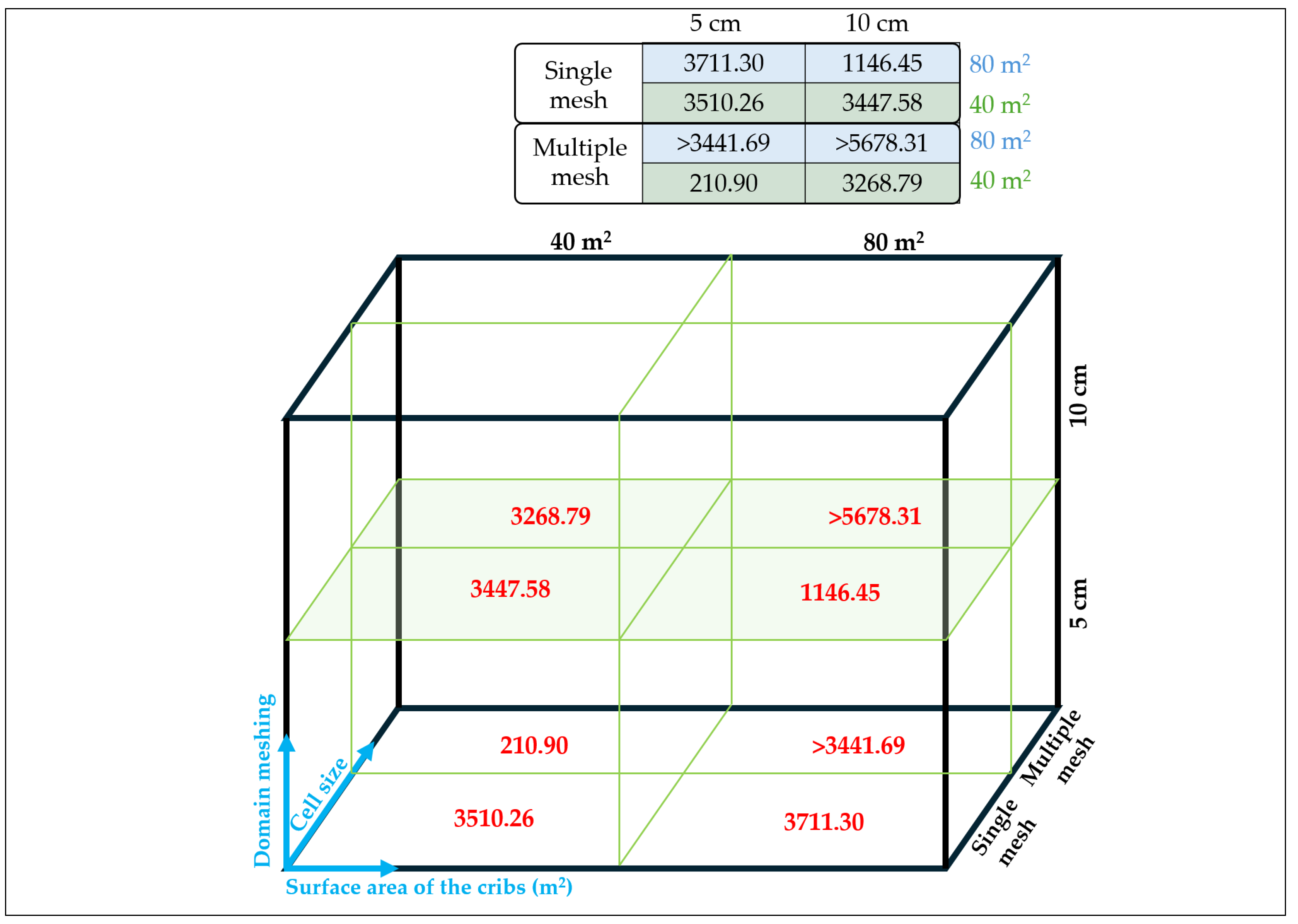
Figure 1. Wood crib dimensions.
Applsci 15 06909 g001
Figure 2. Experimental stand: (a) left view; (b) front view; (c) interior view.
Applsci 15 06909 g002
Figure 3. Three-dimensional scheme of thermocouple positions on distinct measurement layers.
Applsci 15 06909 g003
Figure 4. Top view section of the experimental set-up.
Applsci 15 06909 g004
Figure 5. Time-lapse of fire propagation in the wood cribs.
Applsci 15 06909 g005
Figure 6. Temperature evolution at various heights.
Applsci 15 06909 g006
Figure 7. Experimental fire development: flashover conditions (a) and external flame spread (b).
Applsci 15 06909 g007
Figure 8. Realistic view of the geometry (a); wireframe view of the geometry (b).
Applsci 15 06909 g008
Figure 9. Simulation domain (left side) and burner subdomains (right side).
Applsci 15 06909 g009
Figure 10. Simulation of Office Fire Dynamics.
Applsci 15 06909 g010
Figure 11. Vertical temperature distribution.
Applsci 15 06909 g011
Figure 12. Horizontal temperature distribution.
Applsci 15 06909 g012
Figure 13. Horizontal velocity distribution.
Applsci 15 06909 g013
Figure 14. Oxygen, carbon monoxide and dioxide concentration variation inside the stand.
Applsci 15 06909 g014
Figure 15. RMSE matrix for various simulation configurations.
Applsci 15 06909 g015
Figure 16. Calibration based on HRR.
Applsci 15 06909 g016
Figure 17. Comparison of the corrected average temperatures resulting from the experiment and simulation.
Applsci 15 06909 g017
Figure 18. Vertical temperature gradient and model accuracy: experiment vs. simulation during fire development phases.
Applsci 15 06909 g018
Table 1. Objectives of the domain refinement analysis.
Input DataOutput Data
Domain meshing typeResult Precision
Cell sizeCalculation Processing Time
Surface area of the cribs
Table 2. Calibration based on average error of the temperatures.
Average Values Compared (0–1280 s)
TC names (°C)T1T2T3T4T5T6T7T8T9T10T11T12T13T14
Experiment626.2595.8635.9548.9455.4671.5607.4535.6480.9631.3524.0565.7466.4666.7
Simulation624.9626.6568.9490.2433.8624.9587.0515.4460.3369.6337.0401.3316.1613.7
Average
error
0.2%4.9%11.8%12.0%5.0%7.5%3.5%3.9%4.5%70.8%55.5%41.0%47.5%8.6%
TC names (°C)T15T16T17T18T19T20T21T22T23T24T25T26T27
Experiment644.6644.9604.2673.8647.5602.6653.4665.5603.4646.7611.4596.4435.6
Simulation626.7626.5695.8650.4683.0682.6643.8620.2653.0614.5687.4624.0552.5
Average
error
2.9%2.9%13.2%3.6%5.2%11.7%1.5%7.3%7.6%5.2%11.1%4.4%21.1%
Disclaimer/Publisher’s Note: The statements, opinions and data contained in all publications are solely those of the individual author(s) and contributor(s) and not of MDPI and/or the editor(s). MDPI and/or the editor(s) disclaim responsibility for any injury to people or property resulting from any ideas, methods, instructions or products referred to in the content.

