Slower Ageing of Cross-Frequency Coupling Mechanisms Across Resting-State Networks Is Associated with Better Cognitive Performance in the Picture Priming Task

Abstract

The brain age gap (BAG), the divergence of an individual’s neurobiologically predicted brain age from their chronological age, is a key indicator of brain health. While BAG can be derived from diverse brain metrics, its interpretation often polarizes between early-life trait influences and current state-dependent factors like cognitive decline. Here, we propose an integrative framework that moves beyond single summary statistics by considering the full distribution of brain metrics across regions or time. We distinguish between a neural system’s “baseline” (typical values, e.g., mean) and its “capacity” (extreme values, e.g., maximum) within these distributions. To test this, we analyzed resting-state magnetoencephalography (MEG) from the Cam-CAN adult cohort, focusing on cross-frequency coupling (CFC) within functional MRI-defined networks. We derived network-specific CFC baseline (mean) and capacity (maximum) measures. Separate brain age prediction models were trained for each measure. The resulting BAGs (baseline-BAG and capacity-BAG) for each network were then correlated with cognitive performance on a picture priming task. Both baseline-BAG and capacity-BAG profiles showed associations with cognitive scores, with younger predicted brain age correlating with better performance. However, capacity-BAG exhibited more conclusive relationships, suggesting that metrics reflecting a neural system’s peak operational ability (capacity) may better capture an individual’s current cognitive state. These findings indicate that brain age models emphasizing neural capacity, rather than just baseline activity, could offer a more sensitive lens for understanding the state-dependent aspects of brain ageing.

1. Introduction

The concept of “brain age” has emerged as a valuable tool in neuroscience to quantify an individual’s brain health relative to their chronological age [1]. Typically estimated from neuroimaging or neurophysiological data, predicted brain age serves as a potential biomarker for cognitive status, susceptibility to neurodegenerative diseases, and various psychiatric conditions [2]. The discrepancy between this predicted brain age and an individual’s chronological age is termed the “brain age gap” (BAG) or delta. While BAG offers a compelling index, its interpretation remains a significant challenge, as it may encapsulate both enduring, early-life neurodevelopmental influences and more transient effects of current health or clinical deterioration [3].

Two primary, though not mutually exclusive, perspectives frame the interpretation of BAG: the “state” hypothesis and the “trait” hypothesis [4]. The state hypothesis posits that BAG reflects dynamic, potentially reversible brain function or structure changes linked to an individual’s current physiological or pathological condition. Conversely, the trait hypothesis suggests that BAG is a more stable, enduring characteristic, possibly established early in life and reflecting long-term developmental trajectories or inherent predispositions.

The state hypothesis suggests that an increased brain age gap may indicate brain pathology. For instance, studies have shown that individuals with schizophrenia exhibit a greater brain age gap, which correlates with negative symptom severity, suggesting that the brain age gap could serve as a biomarker for psychosis conversion in high-risk individuals [5]. Alzheimer’s disease (AD) and mild cognitive impairment (MCI) are associated with an increased BAG, indicating accelerated brain ageing. This gap is linked to cognitive impairment and is a predictive marker for disease progression [6]. MRI models have identified higher than control-based brain age for diabetes, multiple sclerosis, mild cognitive impairment, and Alzheimer’s dementia [7]. In another MRI study, neurologically older brains were associated with heavy episodic drinking, higher blood pressure, and higher blood glucose [8].

The trait hypothesis proposes that the brain age gap is a stable, individual characteristic rather than a reflection of transient physiological states [4]. Several studies support this hypothesis, suggesting that the brain age gap primarily reflects inherent individual differences rather than current health conditions or temporary influences [3,4,9].

EEG-based research provides evidence for the trait hypothesis. One study found that the brain age gap does not significantly correlate with pathological EEG changes, suggesting acute neurological abnormalities do not drive it [4]. Another study reported no association between cross-sectional brain age and longitudinal ageing rates [3]. Instead, brain age in adulthood was linked to congenital factors such as birth weight and polygenic scores for brain age, indicating a lifelong influence on brain structure originating in early development.

Additional EEG evidence comes from a study comparing variability in brain age prediction between young and older adults using age prediction models based on middle-aged adults [9]. Greater variability in older adults would be expected due to stochastic accumulation of pathologies, leading to poorer prediction and thus supporting the state hypothesis. However, the study found no significant differences in prediction accuracy between age groups, reinforcing the trait hypothesis.

Studies highlight the overlap between state and trait components in age-related changes in neural irregularity [10]. This irregularity can capture trait-like differences and state-like fluctuations, indicating that brain age may encompass stable and transient elements [11]. Research on functional connectivity shows that state and trait components shape individual differences in brain function. This suggests that while some aspects of brain age are stable, others may vary with mental states [10].

A potential avenue for reconciling the trait and state hypotheses of brain age lies in acknowledging the inherently skewed nature of many neurophysiological parameters. Whether assessed longitudinally or spatially across different regions, brain metrics frequently exhibit distributions more akin to log-normal than Gaussian patterns [12]. This prevalence of skewed, heavy-tailed distributions is not unique to neuroscience. Still, it is a common feature in complex biological systems, particularly for measures constrained to positive values, such as synaptic strengths, neuronal firing rates, or network connectivity [13].

The ubiquity of such distributions in brain organization implies that relying on a single summary statistic, like the mean, can be misleading. In skewed distributions, a small number of high-magnitude observations can disproportionately influence the mean, rendering it an incomplete or even biased descriptor of the system’s central tendency or typical state. For instance, the average firing rate of a neuronal population can be heavily skewed by a minority of hyperactive neurons, even if most neurons fire at much lower rates [13]. Consequently, brain age estimates derived from metrics of local or coordinated neural activity might be unduly influenced by extreme values in a specific subset of brain regions or during particular epochs, rather than reflecting a homogenous process across the entire brain or consistently over time [12]. This suggests that different aspects of these skewed distributions, such as the typical value versus the extreme tail, might capture distinct facets of brain function relevant to the trait versus state interpretations of brain age.

We propose that the central mode and the tail of skewed distributions represent two complementary aspects of the same neural dynamics: a baseline reflecting typical values and an indicator of the system’s overall capacity [14]. Functional parameters in biological systems, including neural networks in the brain, often exhibit a wide dynamic range, enabling adaptation to varying demands [15]. The most representative values, such as the mean or median of a parameter measured across time or brain regions, primarily capture the system’s typical operation under normal conditions. However, these central tendencies may overlook critical differences that emerge under extreme conditions, such as peak cognitive demand, stress, or pathology [16].

The right tail of skewed distributions, representing the observed values of a brain parameter beyond the central tendency, may provide insight into the system’s transient effects, which in turn may reflect reserve capacity [17]. In the context of neural activity, this could correspond to the maximal firing rates of a subset of neurons, the peak amplitude of evoked responses, or the highest levels of functional connectivity observed under demanding conditions [18]. These extreme values may represent the system’s upper limits, revealing potential vulnerabilities or resilience in response to physiological or pathological challenges. One example demonstrating the idea of neural capacity is the concept of cognitive reserve.

We further propose that the distinction between the trait and state hypotheses can be reframed in terms of a neural network’s baseline function and its capacity. Specifically, we propose that the baseline represents the system’s typical operation under normal conditions, while extreme event dynamics reflect the dynamic repertoire of brain states [19]. We hypothesize that the baseline, characterized by the most representative values of neural activity, is primarily shaped by stable, individual-specific factors established early in life. In contrast, extreme neural dynamics, captured by the distribution’s right tail, reflect the system’s capacity to adapt to challenges, such as cognitive load, stress, or pathological disruptions. These fluctuations in peak activity or network efficiency may provide a more sensitive window into the current state of the neural system.

Our study illustrates how neural networks’ baseline and capacity contribute to brain age prediction and their associations with cognitive performance. We specifically test whether the brain age gap, computed separately for these two aspects of skewed distributions, relates to cognitive function. To investigate this, we analyze a large cohort of adults spanning a wide age range from the Cam-CAN study. We use resting-state magnetoencephalography (MEG) data and cognitive performance across multiple domains. We analyze neural networks based on how they are defined in the literature on resting-state functional magnetic resonance imaging (rs-fMRI). For each brain region of interest (ROI) defined by a cortical parcellation as our primary brain metric, we compute cross-frequency coupling (CFC), a key mechanism for coordinating brain rhythms. We define the baseline function for each network as the typical CFC value across ROIs within the given network, representing the system’s normal operational range.

In contrast, we define capacity as the maximum CFC value within the same network, reflecting its upper functional limits. We then predict biological age using both baseline and capacity measures of CFC and estimate the brain age gap for each approach. Finally, we examine correlations between these neural metrics and cognitive performance to determine whether baseline and capacity provide distinct insights into cognitive ageing.

2. Methods

2.1. Data Statement

We analyzed data from the Cambridge Centre for Ageing and Neuroscience (Cam-CAN) study [20,21]. This is a large-scale, multidisciplinary research initiative that examines the effects of ageing on brain structure, function, and cognition across the lifespan. Cam-CAN integrates behavioural, neuroimaging (MRI, MEG), and cognitive data from a population-based sample of adults aged 18 to over 88. For this study, we used magnetoencephalography (MEG), structural magnetic resonance imaging (MRI), and psychometric assessments. The psychometric evaluation included seven tasks to measure executive function, working memory, and semantic memory. Our final sample consisted of 447 participants between 18 and 87 years old, with complete data across all required modalities.

Our use of this de-identified MEG, structural MRI, and cognitive data for secondary analysis was approved by the Simon Fraser University Research Ethics Board (Protocol #30001248). This secondary use was determined to present minimal risk to participants as all data were fully anonymized prior to their release by Cam-CAN and their access by our research team.

2.2. Neurophysiological Recordings

Resting-state MEG was recorded with a VectorView MEG scanner (Elekta Neuromag, Helsinki, Finland) with 102 magnetometers and 204 gradiometers and a sampling rate of 1 kHz. The eyes-closed recordings were approximately eight minutes long in a magnetically shielded room. We analyzed the recordings preprocessed from Cam-CAN Release 005. Specifically, the MEG recordings were MaxFiltered (v2.2.12). The MaxFilter algorithm allowed them to remove noise from external sources, provide head movement compensation, and reconstruct noisy channels. For a complete description of the MEG acquisition protocol, refer to Taylor et al., 2017 [21].

To reconstruct neuromagnetic dynamics, we used structural MRI data. The MRI scans were recorded using a 3T Siemens TIM Trio Scanner (Erlangen, Germany) with a 32-channel head coil. The T1-weighted MRI images were obtained using the magnetization-prepared rapid gradient-echo (MP-RAGE) sequence with a repetition time (TR) of 2250 ms, an echo time (TE) of 2.99 ms, and a flip angle of 9°. The field of view was 256 × 240 × 192 mm³, with an isotropic voxel size of 1 mm in all directions. For further details on the MRI acquisition protocol, refer to Taylor et al., 2017 [21].

2.3. Psychometrics

From the initial Cam-CAN cohort of 652 participants with available MEG/MRI data, our preprocessing pipeline yielded successful source reconstructions for 605 individuals (296 females, 309 males). This group was then cross-referenced with available cognitive assessments. After excluding additional participants who lacked complete cognitive score data, our final sample for analysis comprised 447 participants (211 females, 236 males).

Participants completed cognitive tests assessing multiple domains, including executive function, short-term memory, semantic memory, and somatosensory function [20]. Each test included multiple metrics capturing different aspects of cognitive performance. To ensure data completeness, we selected only tests with available data for at least two-thirds of participants who also had neuroimaging data. This selection yielded 8 cognitive tests, comprising 21 total performance metrics, for 447 participants. The selected tasks included the colour wheel task, hotel task, picture priming task, reaction time choice task, simple reaction time task, tip-of-the-tongue task, proverbs task, and famous faces task.

Table 1. Cognitive test measurement names and short descriptions, as defined in the original Cam_CAN study [20,21].

Name of Measurement	Description
Tip-of-tongue—Ratio	The ratio of the total number of tip-of-tongue occurrences divided by the total number of faces the participants say they can recognize
Picture Priming—High semantic priming effect	Effect of high semantic priming on reaction time
Picture Priming—High phonetic priming effect	Effect of high phonetic priming on reaction time
Picture Priming—Low semantic priming difference	Change in naming accuracy between baseline and low semantic priming
Picture Priming—High semantic priming difference	Change in naming accuracy between baseline and high semantic priming
Picture Priming—Low phonetic priming difference	Change in naming accuracy between baseline and low phonological priming
Picture Priming—High phonetic priming difference	Change in naming accuracy between baseline and high phonological priming
Picture Priming—Number recall	Total number across all conditions where participant names the image correctly with a correct reaction time (>200 ms)
Simple Reaction Time—Median	The median reaction time of correct responses
Simple Reaction Time—Mean	The mean reaction time of correct responses
Simple Reaction Time—Accuracy %	The percentage of button presses where the participant correctly used their index finger
Reaction Time Choice—Median	The median reaction time of correct responses
Reaction Time Choice—Mean	The mean reaction time of correct responses
Reaction Time Choice—Accuracy %	The accuracy of pressing a button with the correct finger (each finger is on one of 4 buttons)
Proverbs—Score	Rating of participant’s explanation of English proverbs (range of 0–2)
Hotel—Total delta time	The summed total deviation from the allotted 2 min to complete each one of 5 tasks
Hotel—Number tasks completed	The number of tasks completed out of 5
Colours—Colour recall	The accuracy of the colour selected by participants after being presented with a randomly determined number of color discs, ranging from 1 to 4.
Faces—Familiar recall %	The percentage of faces of public figures that are familiar with the number of expected responses
Faces—Occupation recall %	The percentage of faces of public figures where participants can recall occupation over the number of expected responses
Faces—Name recall %	The percentage of faces of public figures where participants can recall their name over the number of expected responses

provides a complete list and description of the test metrics.

For further analysis, we normalized each cognitive score to a mean of zero and a variance of one. Some metrics, such as reaction time, were inversely related to performance, with lower values indicating better outcomes. To ensure consistency in brain–behaviour correlations, we inverted these metrics by multiplying their values by −1, so that higher scores consistently reflected better performance.

2.4. MEG Preprocessing

The preparation of MEG data for further analysis involved several key stages, including preprocessing and reconstructing neuromagnetic dynamics in brain space. We preprocessed the Max-Filtered MEG recordings from the Cam-CAN dataset as follows. First, we removed the initial 30 s of each recording to exclude potential transient artefacts, then extracted a uniform one-minute segment for each participant. We followed the preprocessing workflow established in previous studies that analyzed the Cam-CAN data algorithms [22]. For MEG preprocessing and subsequent source reconstruction, we used algorithms implemented in the MNE-Python toolbox [23].

We bandpass filtered the signals between 1 Hz and 90 Hz and downsampled the data to 512 Hz. To remove electrooculography (EOG) and electrocardiography (ECG) artefacts, we applied independent component analysis (ICA). Using the ‘Picard’ method with 40 components, we detected eye blink and heartbeat interference by correlating the components with the EOG and ECG channels, respectively. The MNE-Python methods (Version 1.7), find_bads_eog() and find_bads_ecg(), were used to identify components strongly correlated with EOG and ECG signals based on default parameters for the correlation threshold [24].

2.5. Neuromagnetic Source Reconstruction

To estimate cortical source activity from sensor-level MEG data, we applied a linearly constrained minimum variance (LCMV) beamformer [25,26] implemented in MNE-Python. The reconstruction process involved several key steps.

First, the MRI and MEG coordinate systems were co-registered for each participant using anatomical landmarks to generate a transformation matrix. The individual’s cortical surface was reconstructed from T1-weighted MR images using the FreeSurfer recon-all algorithm [27,28,29]. This process yielded a boundary element model (BEM) and defined the source space at an oct6 resolution.

Second, a forward solution, modelling the contribution of each cortical source to the MEG sensor signals, was computed using MNE-Python’s make_forward_solution() function. This step integrated the co-registration transformation, the oct6 surface mesh (serving as the source model), the BEM, and preprocessed MEG metadata. To ensure consistent source orientation across participants, the forward solution was subsequently converted to have fixed orientations normal to the cortical surface using convert_forward_solution() with the surf_ori=True and force_fixed=True parameters.

Third, the LCMV beamformer was then applied to the preprocessed MEG data using the make_lcmv() and apply_lcmv_raw() functions to reconstruct neuromagnetic source activity across the oct6 cortical mesh. To obtain representative dynamics for functionally defined regions, we applied the Schaefer 400-region cortical parcellation atlas [30], which segments the cortex into regions of interest (ROIs), which are aligned with large-scale intrinsic connectivity networks identified from resting-state functional MRI [31] and assigns each of the 400 ROIs (200 per hemisphere) to one of 17 established functional networks. For each of these 400 ROIs, a single representative time course was extracted using MNE-Python’s () extract_label_time_course() function with the mode=‘mean_flip’ parameter. This method averages activity across vertices within an ROI after aligning their orientations by flipping the sign of time series at vertices whose orientation deviates by more than 90° from the dominant orientation within that ROI.

This pipeline resulted in estimating neuromagnetic dynamics for each participant at 400 functionally defined cortical locations, corresponding to the Schaefer atlas parcellation.

2.6. Cross-Frequency Coupling

We computed cross-frequency coupling (CFC) matrices for each participant to characterize the interaction between neural oscillations at different frequencies [32,33]. CFC facilitates information integration across brain regions and timescales and plays a key role in cognitive functions such as memory, perception, attention, and motor control [34]. Various methods exist to quantify CFC [32]. In our study, we focused on phase–amplitude coupling (PAC), which measures how the phase of a slow oscillation modulates the amplitude of a faster oscillation [35,36].

We computed a 20 × 30 PAC matrix for each of the 400 ROIs defined by the Schaefer parcellation. This matrix represents the interaction between 20 low-frequency oscillations (1–12 Hz) and 30 high-frequency oscillations (13–75 Hz). Using a time-frequency decomposition, we reconstructed single-source MEG dynamics at these frequency points evenly spaced on a logarithmic scale. We applied an eighth-order complex Gaussian derivative wavelet to reconstruct the analytic signal for each wavelet frequency [37]. We then computed the instantaneous phase of low-frequency signals and the amplitude envelope of high-frequency signals.

After calculating low-frequency phases and high-frequency amplitudes, we estimated the normalized modulation index (MI) for each phase–amplitude frequency pair. The normalized MI quantifies the coupling strength while accounting for signal amplitude, ensuring participant comparability.

As a result of this procedure, each participant was characterized by 400 ROIs, with each ROI associated with a 20 × 30 PAC matrix. Each ROI was assigned to one of 17 functional networks, separately for the left and right hemispheres, yielding a total of 34 network-based classifications.

2.7. Mean and Maximum Values of Cross-Frequency Coupling

We characterized each functional network using two parameters: baseline cross-frequency coupling (CFC) and CFC capacity. Each network consisted of multiple regions of interest (ROIs). We computed the median phase–amplitude coupling (PAC) across all ROIs within a given network to quantify baseline coordinated activity. We calculated the maximum PAC value across ROIs within the same network to assess CFC capacity.

This procedure resulted in 34 functional networks per participant, represented by two 20 × 30 PAC matrices. One matrix reflected the network’s baseline CFC, while the other represented its capacity to sustain phase–amplitude coupling. We used these network-level metrics in subsequent analyses to predict participants’ age.

2.8. Brain Age Gap Based on Cross-Frequency Coupling

We predicted brain age and estimated the brain age gap separately for each of the 34 functional networks, considering the baseline and capacity cross-frequency coupling (CFC) metrics separately. To predict brain age from cross-frequency phase–amplitude coupling (PAC) features, we employed Relevance Vector Regression (RVR), a sparse Bayesian machine learning method [38]. While sharing operational principles with Support Vector Regression (SVR), RVR incorporates probabilistic inference, typically yielding a more parsimonious model that uses fewer input features (or “relevance vectors”) and is less prone to overfitting. In this study, the RVR model was trained using these CFC features derived from all participants, with chronological age as the target variable for prediction. The analysis was performed using the sklearn-rvm Python package, with the RVR configured to use a polynomial kernel of degree 3.

To estimate the brain age gap for each network and CFC metric, we used 10-fold cross-validation. We divided participants into ten equal groups, trained the model on 90% of the data, and tested it on the remaining 10%. This process was repeated ten times, ensuring that each participant’s brain age was predicted without their data being included in the training set.

After obtaining brain age predictions, we retained only the networks that showed robust associations with chronological age. We computed a distance correlation t-test for each network between chronological and predicted age using the distance_correlation_t_test() function from the dcor Python package [39]. We corrected network-specific p-values for multiple comparisons using a false discovery rate (FDR) threshold of 5%. In subsequent analyses examining correlations between the brain age gap and psychometric performance, we included only those functional networks where predicted age showed a robust correlation with chronological age.

We computed the brain age gap (BAG) for each selected functional network as the deviation of a participant’s predicted brain age from the population average. Specifically, we applied a quadratic regression for each CFC metric and functional network to model the relationship between chronological age and predicted brain age. We then calculated the BAG for each participant by subtracting the predicted brain age from the regression-based population average.

Positive BAG values indicated slower ageing, meaning that the participant’s cross-frequency coupling profile resembled a younger individual’s. Conversely, negative BAG values reflected accelerated ageing, where the participant’s CFC profile appeared older than expected for their chronological age. Each participant was ultimately characterized by two sets of network-specific brain age gap estimates, one for each CFC metric. Notably, the same participant could exhibit both accelerated and slowed ageing effects across different functional networks.

2.9. Associations Between Brain Age Gap and Psychometrics

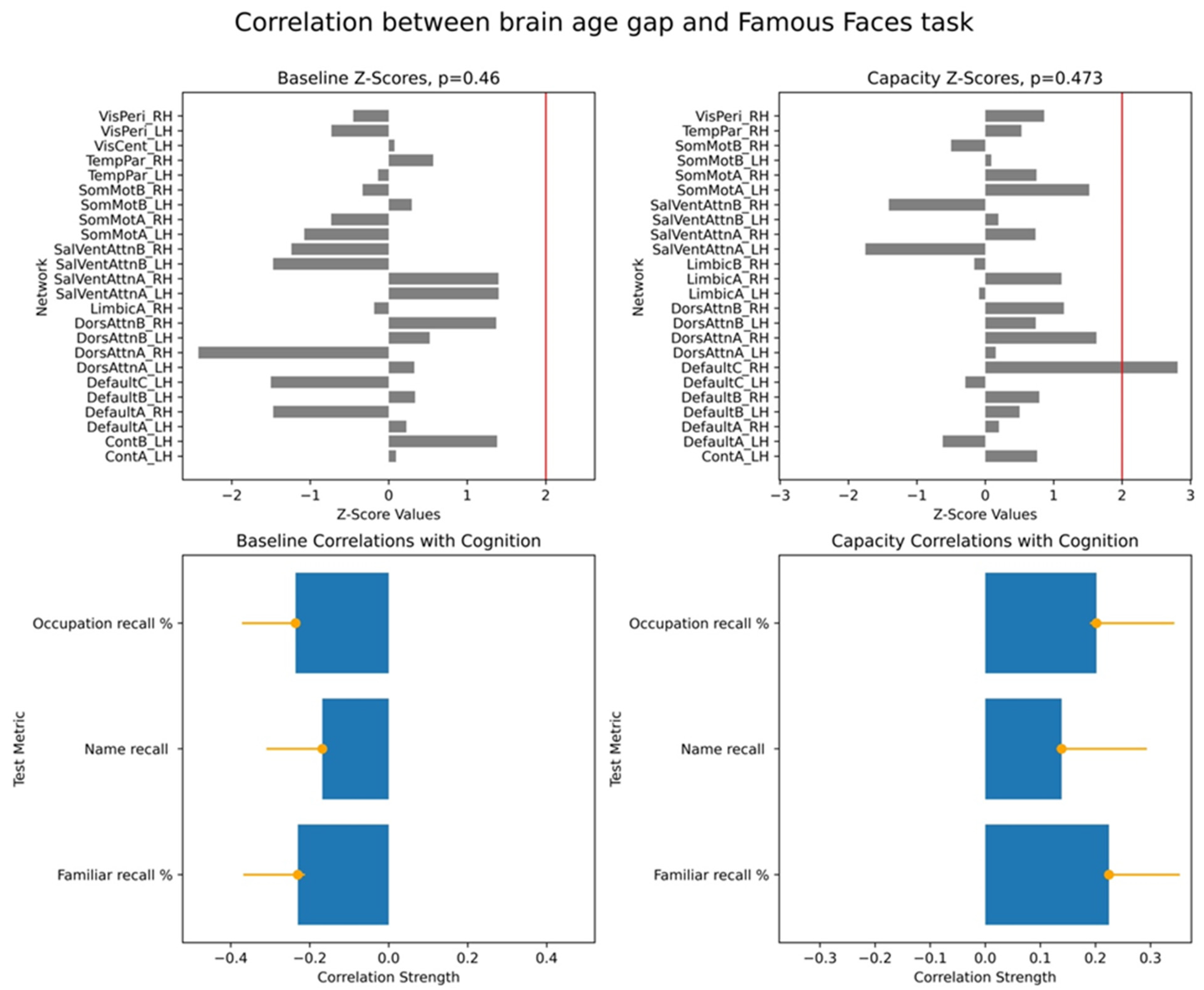
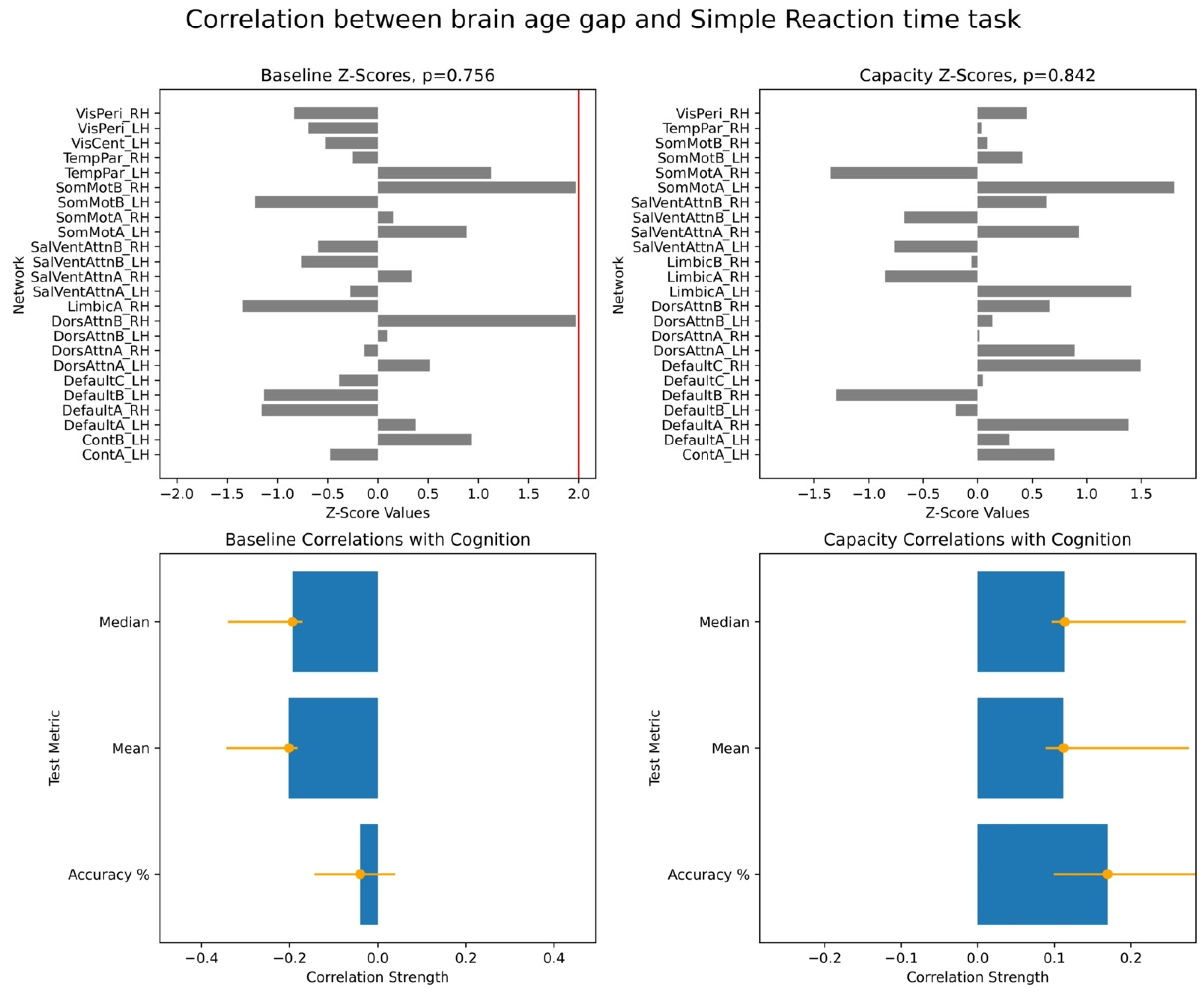
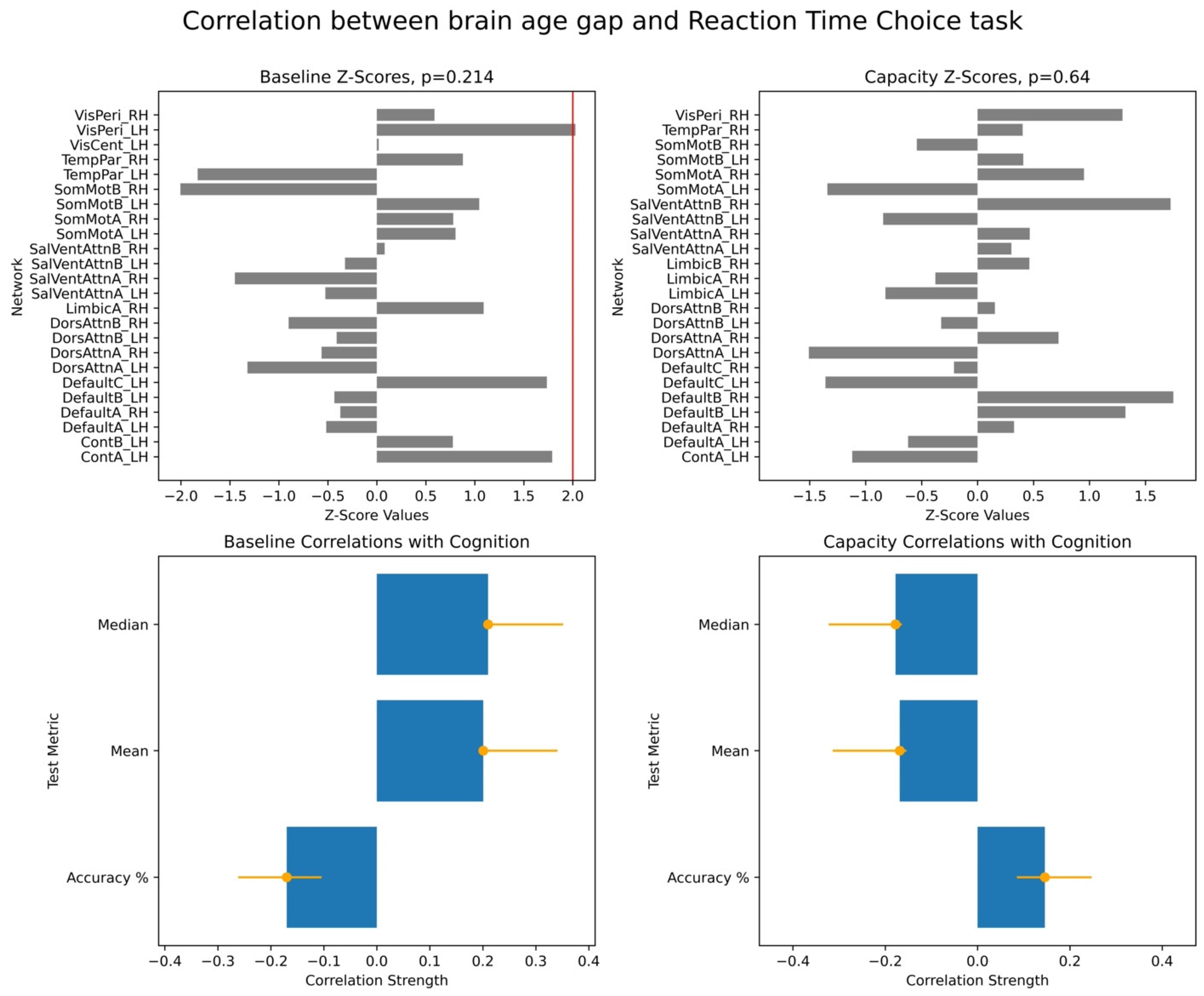
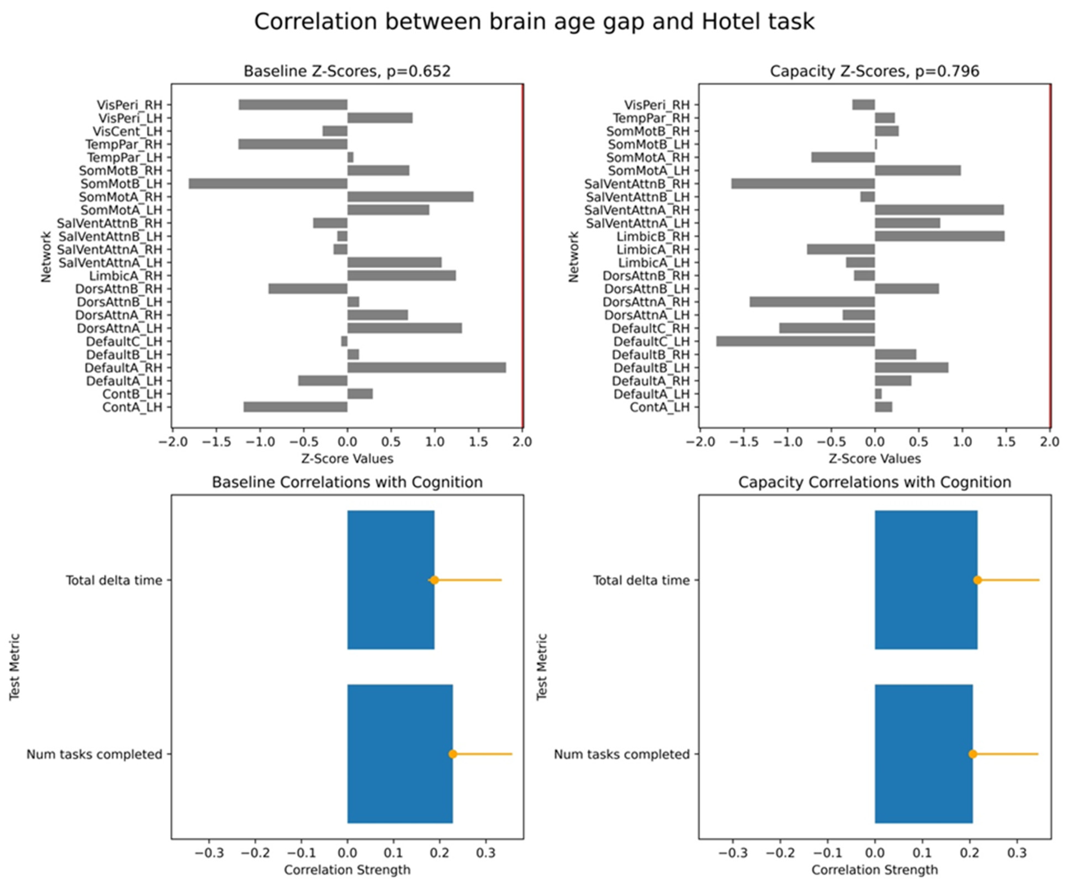
In the final analysis stage, we examined correlations between brain age gap (BAG) estimates and cognitive performance. We applied behavioural partial least squares (PLS), a multivariate technique commonly used in neuroimaging to assess brain–behaviour relationships [40,41,42,43]. This analysis was conducted separately for each of the two BAG profiles and each cognitive test, resulting in 16 Behavioural PLS analyses (2 BAG profiles × 8 cognitive tests).

Behavioural PLS decomposed the covariance between network-specific BAG estimates and cognitive scores into latent variables (LVs) using singular value decomposition (SVD). Each LV captured a distinct pattern of covariance between brain age gaps and cognitive performance across participants.

To assess the significance of the overall brain–cognition correlations, we performed a permutation test wherein we randomly shuffled data across participants and tested for stability of correlations based on the original data. This produced a vector of overall correlations, with dimensionality determined by the number of cognitive scores. We performed a bootstrap test to evaluate the robustness of individual networks’ contributions to the identified overall correlations. In each bootstrap iteration, we resampled participants with replacements while preserving the correspondence between each participant’s BAG and cognitive scores. Behavioural PLS then computed bootstrap ratio values, defined as the ratio of original network saliences to the standard error of the bootstrap distribution. These values are equivalent to z-scores. In our study, we used the terms of bootstrap ratio values and z-scores interchangeably. We applied 10,000 iterations for both permutation and bootstrap tests and focused on the first LV, which accounted for the largest proportion of variance in the brain–cognition covariances.

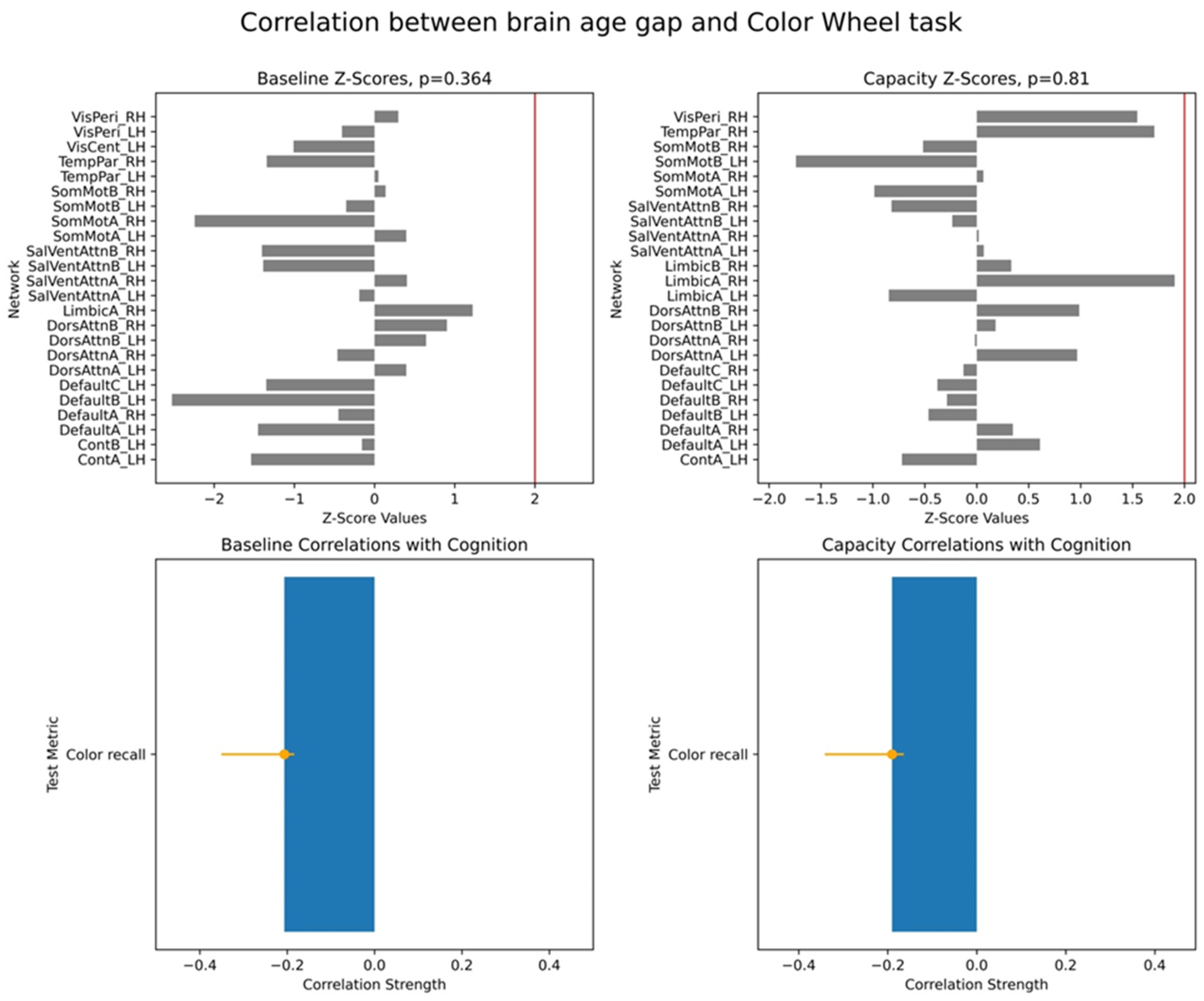
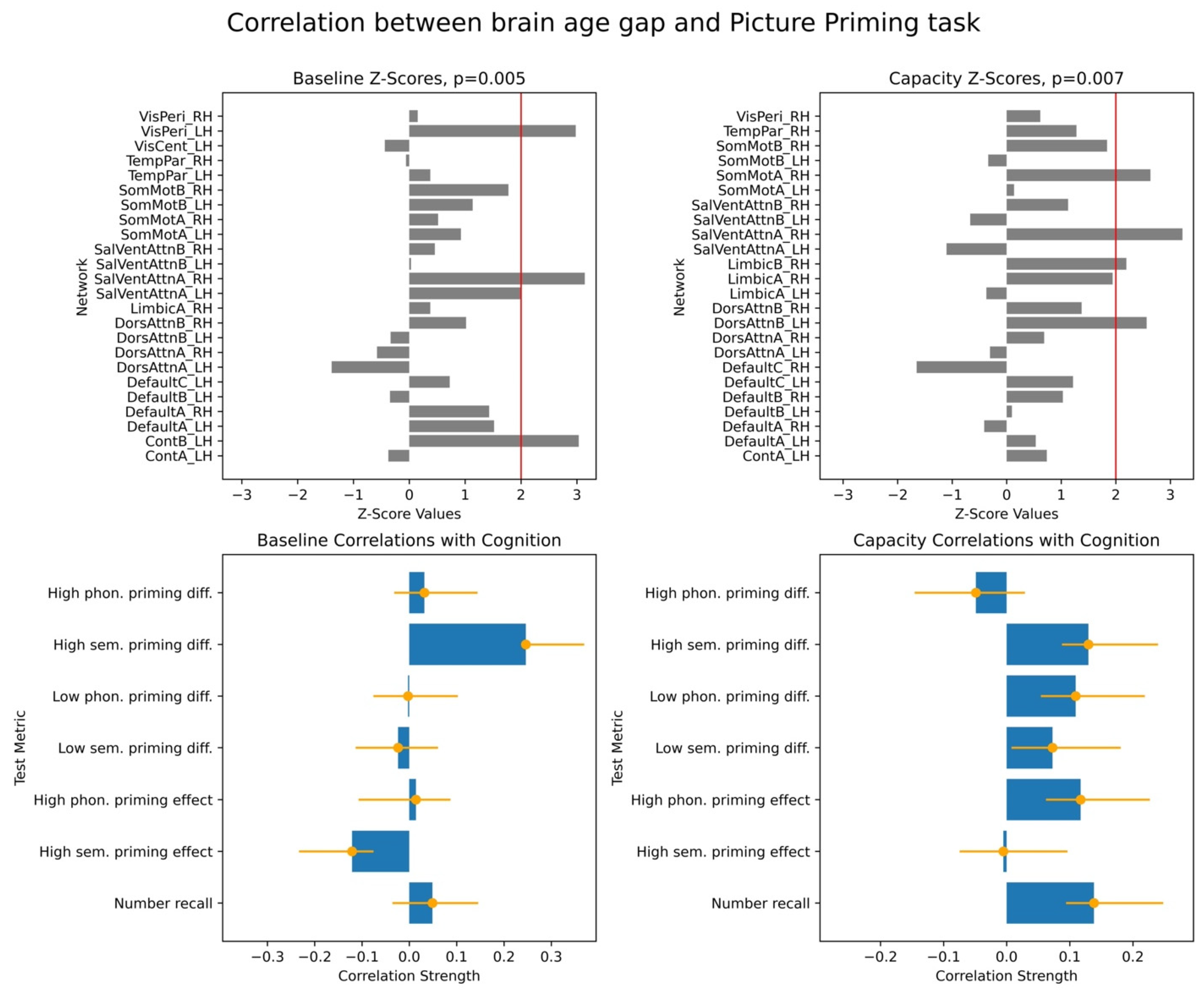
For each PLS analysis, we reported three key results: (i) a vector of overall correlations, with each value representing the association between BAG and a cognitive variable within a given test; (ii) a p-value assessing the statistical significance of these correlations across the entire dataset; and (iii) a vector of network-specific z-scores, indicating the robustness of networks’ contribution to the observed brain–cognition overall correlations, as defined in (i). Larger absolute z-scores reflected more potent effects, and we focused on networks with z-scores greater than ±2, approximately corresponding to a 95% confidence interval.

We note that PLS analysis yields several metrics for interpreting brain–behaviour relationships. First, it provides a global significance value for each identified latent variable (LV), which represents the strength of the overall multivariate correlation between the combined imaging features and behavioural scores. The individual correlation values between the cognitive scores and the LV’s brain scores indicate the effect size concerning specific behavioural outcomes. For the imaging data, the contribution of individual fMRI networks to the LV is quantified using Z-scores, which are computed as bootstrap ratio values. These ratios are derived by dividing the original salience of each network by the standard deviation of its bootstrap distribution, thereby providing a measure of effect size for each network’s involvement in the identified pattern.

Interpretation of individual correlations between BAG and cognitive scores required considering overall correlations and z-scores together. Positive brain–cognition associations were reflected either by both a positive overall correlation and z-score or by both values being negative. Conversely, negative brain–cognition associations occurred when one metric (correlation or z-score) was positive and the other was negative.

3. Results

For both profiles of network-specific brain age gaps, we identified 24 networks, which expressed robust associations between predicted and chronological age. 20 networks were common for both profiles: ‘DorsAttnB_LH’, ‘ContA_LH’, ‘VisPeri_RH’, ‘SomMotA_RH’, ‘DefaultA_RH’, ‘SalVentAttnB_RH’, ‘DefaultA_LH’, ‘SalVentAttnB_LH’, ‘DorsAttnB_RH’, ‘SomMotA_LH’, ‘SomMotB_LH’, ‘DorsAttnA_RH’, ‘SalVentAttnA_LH’, ‘DefaultB_LH’, ‘SalVentAttnA_RH’, ‘SomMotB_RH’, ‘DorsAttnA_LH’, ‘LimbicA_RH’, ‘DefaultC_LH’, ‘TempPar_RH’. The labels’ LH’ and ‘RH’ indicate the reference to the left and right hemisphere, respectively. Four networks were unique for the baseline-related metric: ‘VisPeri_LH’, ‘ContB_LH’, ‘VisCent_LH’, ‘TempPar_LH’. Also, four networks were unique for the capacity-based metric: ‘DefaultB_RH’, ‘DefaultC_RH’, ‘LimbicA_LH’, ‘LimbicA_LH’. We applied a series of multivariate analyses (behavioural PLS) to explore correlations between brain age gap and cognitive test performance.

3.1. Picture Priming Task

Partial least squares (PLS) analysis revealed a significant overall relationship between brain age gap (BAG) and cognitive performance on one specific cognitive test, the Picture Priming Task (overall p < 0.05). Figure 1 displays the results of two separate PLS analyses for this task, one for BAG derived from baseline cross-frequency coupling (CFC) metrics (left column) and another for BAG derived from capacity CFC metrics (right column). In each column, the lower plot shows the overall correlation coefficients between BAG and individual cognitive scales from the Picture Priming Task, while the upper plot shows the corresponding bootstrap ratios (Z-scores) for each functional network’s contribution to this relationship.

For both baseline-based and capacity-based BAG analyses, the distributions of network Z-scores (Figure 1, upper plots) were predominantly positive, indicating a consistent directionality of network contributions to the overall PLS effect. We focused on networks with Z-scores exceeding 2, signifying robust contributions. Four such networks were identified for the baseline-CFC BAG, and four for the capacity-CFC BAG. The consistently positive Z-scores allow for a direct interpretation of the brain–behaviour relationships based on the sign of the overall correlation coefficients (Figure 1, lower plots).

Examining the baseline CFC-derived BAG (Figure 1, left column), the pattern of correlations with cognitive scales from the Picture Priming Task was mixed. For instance, BAG positively correlated with lower semantic priming difference scores but negatively correlated with lower phonetic priming difference scores. This heterogeneity in the direction of effects did not yield a clear, unidirectional relationship between baseline-BAG and cognitive performance, suggesting that both positive (slower ageing) and negative (accelerated ageing) BAG values could be associated with better performance on different aspects of the task.

In contrast, the capacity CFC-derived BAG (Figure 1, right column) exhibited a qualitatively distinct and more consistent pattern. Specifically, BAG derived from CFC capacity measures showed positive correlations with five out of the seven cognitive scales of the Picture Priming Task. Given that a positive BAG indicates a brain appearing younger than its chronological age (i.e., slower ageing) and positive values on these cognitive scales represent better performance, this pattern consistently suggests that slower brain ageing, as indexed by capacity-BAG, is associated with enhanced cognitive function on this task. This consistent relationship was supported by the predominantly positive network-level Z-scores.

3.2. Other Cognitive Tasks

No statistically significant overall relationships were found between the brain age gap (BAG) and cognitive scores for the remaining cognitive tasks included in our analyses. All p-values derived from the partial least squares (PLS) analyses for these tasks ranged between 0.15 and 0.81. The full results of these non-significant PLS analyses are presented in Figure A1, Figure A2, Figure A3, Figure A4, Figure A5, Figure A6 and Figure A7 for transparency and completeness. These appendix figures adhere to the same format as Figure 1, illustrating the overall correlation coefficients and network-specific Z-scores for each task, though none achieved statistical significance, as tested by a series of PLS analyses.

4. Discussion

In our study, we explored the utility of the brain age gap (BAG), which is the difference between an individual’s neurobiologically predicted age and chronological age, as a lens to understand cognitive ageing. Conventionally, a positive BAG implies a brain appearing “younger” than its chronological age, whereas a negative BAG suggests accelerated brain ageing. While brain age can be derived from diverse neurophysiological measures, our approach centred on cross-frequency coupling (CFC). This choice was motivated by CFC’s critical role in orchestrating neural oscillations across multiple timescales within brain regions, providing a sensitive measure of coordinated neural dynamics relevant to ageing and cognitive function.

We estimated brain age separately for a collection of neural networks defined a priori using a functional parcellation of resting-state fMRI networks [30,31]. Critically, we reconstructed two distinct profiles of brain age. In one approach, we predicted chronological age using CFC averaged across regions of interest (ROIs) within each network, representing the network’s baseline activity. In the second approach, we used the maximum CFC value across ROIs within the same network, reflecting the network’s capacity to generate strongly coupled temporal activity. These two profiles of network-specific brain age gap estimates capture different aspects of neural dynamics: baseline levels of functional coupling and the potential for extreme neural synchronization across frequencies.

Finally, we examined associations between these two brain age profiles and participants’ cognitive performance, measured across eight tasks assessing working memory, executive function, and semantic memory. We found robust positive correlations between the capacity-based brain age gap and scores on the picture priming task, which reflects semantic memory. In contrast, results for the baseline-based brain age in the same task were inconclusive. Our findings align with the hypothesis that the brain age gap reflects an individual’s current cognitive state, supporting the state hypothesis of brain ageing.

Our overall rationale for distinguishing two types of cross-frequency coupling was based on the observation that brain parameters commonly exhibit skewed distributions [44]. This pattern is prevalent across multiple levels of neural hierarchy and closely resembles log-normal distributions [13]. In our interpretation of the brain age gap, we specifically analyzed these distributions’ central mode and right tail, focusing on variability within functional networks.

We computed the maximum cross-frequency coupling (CFC) within each network to characterize extreme values. While multiple approaches exist for quantifying distribution tails, statistical properties such as skewness and kurtosis, among other metrics, could also provide meaningful insights into cognitive and clinical states.

Skewness effectively differentiates cognitive states such as meditation, mathematical problem-solving, and open-eye conditions, making it a versatile metric for cognitive state monitoring [45]. Similarly, kurtosis has demonstrated clinical relevance across various domains. In pediatric epilepsy, high-frequency brain signals show significantly elevated kurtosis in epileptogenic zones compared to controls [46]. In neurodegenerative disorders, EEG studies of Alzheimer’s patients report increased kurtosis values, which have contributed to the development of kurtosis-based denoising techniques that enhance diagnostic accuracy [47]. Additionally, brain–computer interface (BCI) research has leveraged kurtosis to classify motor imagery tasks in EEG data, achieving high accuracy in distinguishing between imagined left- and right-hand movements [48].

A study using resting-state MEG data from the Cam-CAN dataset further demonstrated the relevance of extreme values in characterizing age-related changes in neural activity [49]. By analyzing frequency-specific signal amplitudes in terms of skewness and kurtosis, the study described how these statistical features captured the variability of neural dynamics across the lifespan. Similarly, another study used resting-state EEG to predict Fugl-Meyer upper extremity motor scores in individuals with chronic stroke [50]. With functional connectivity estimated as the mean and maximum phase-locking value, the study found that maximum-based estimates achieved higher prediction accuracy [50]. These findings reinforce the importance of considering distribution tails when interpreting neural metrics.

Characterizing the tails of the skewed distributions and focusing on their maximum values, skewness, or kurtosis falls into the domain of extreme value theory (EVT). In neural networks, EVT can be used to evaluate robustness against adversarial examples [51]. The extreme events help assess neural networks’ capacity to resist extreme perturbations, thereby defining their robustness and capacity. In a study exploring the interaction between olfactory and visual systems in vertebrates, EVT was applied to model cross-modal sensory information integration [14]. This integration was mediated by extreme responses rather than average cell responses, suggesting that neural capacity is influenced by the ability to handle extreme sensory inputs.

Cross-frequency coupling (CFC) in neural ensembles requires understanding how different oscillatory frequencies interact to enhance cognitive processes such as memory, perception, and attention [34]. CFC is a mechanism by which neural oscillations at different frequencies synchronize, facilitating information integration across neural populations [33]. This coupling is crucial for robust information storage and retrieval and for the modulation of cognitive functions [52].

Our study has limitations. We recognize that using the maximum value of cross-frequency coupling across brain regions to represent neural network capacity is a simplification. From a theoretical perspective, interpreting this peak, or the upper tail of its distribution, as a direct measure of neural capacity currently lacks strong theoretical grounding. CFC can occur through various mechanisms, including phase-phase and phase–amplitude coupling, which are influenced by synaptic time scales, synaptic coupling, and neural population excitability [32]. Inhibitory neural mass models demonstrate that CFC can emerge from the collective dynamics of neural populations, with different dynamical regimes such as periodic and quasi-periodic oscillations [53]. Nonlinear interactions in neural fields, rather than specialized cells, can generate CFC, suggesting a universal mechanism across multi-scale systems [54].

Neuronal ensembles are considered modular units of neural circuits [55]. Neuronal ensembles represent and process information through coordinated activity patterns, which are influenced by factors such as the size of the ensemble, the diversity of neuronal responses, and the synaptic connections within the ensemble [55]. The capacity of a neural ensemble can be conceptualized in terms of its ability to encode, store, and retrieve patterns or information, which is influenced by the structure and dynamics of the neuronal ensemble. For example, cross-frequency coupling, particularly between theta and gamma oscillations, has been shown to increase the memory capacity of neural networks [56].

Other limitations should be acknowledged. First, although we analyzed a broad range of cognitive assessments available within the Cam-CAN dataset, our analyses did not incorporate all potentially influential variables. Factors such as detailed educational history, comprehensive health status indicators beyond gross clinical categories, and specific lifestyle variables (e.g., diet, physical activity) were not included. The inclusion of such covariates could further refine our models of brain–behaviour relationships and potentially reveal nuances in the observed effects or identify moderating influences.

Second, our investigation of brain network dynamics relied on specific, well-established cortical parcellations [30,31]. While these atlases are prevalent in functional MRI research, facilitating comparability with the vast body of existing literature, they represent only a subset of available parcellation schemes. These parcellation, while foundational, is now relatively dated [57]. Using additional or more contemporary atlases, potentially derived from different modalities or based on different organizational principles, could offer further insights into the robustness and generalizability of our findings across various network definitions.

Third, in our cross-frequency coupling (CFC) analysis, we focused on mean values and metrics reflecting the upper tail of the distribution (i.e., maximum values). This decision was motivated by the observation that neurophysiological measures often exhibit skewed distributions where the mean alone provides an incomplete representation, potentially obscuring functionally relevant extreme values [13]. While we interpret these as speculatively representing baseline and peak coupling capacity, respectively, this is a simplification. A more exhaustive characterization of the entire CFC distribution, or the exploration of alternative metrics beyond the mean and maximum, could provide a more nuanced understanding of CFC dynamics. Future studies could also benefit from explicitly modelling the skewness or other distributional properties [49].

The observed correlation between the brain age gap derived from the cross-frequency coupling (CFC) and performance specifically on the picture priming task, but not other cognitive tasks, warrants further consideration. While the precise reasons for this specificity remain fully elucidated, the neurophysiological underpinnings of picture priming offer plausible explanations. Picture priming tasks rely on the efficient processing and integration of visual object information, processes known to involve coordinated activity across several brain regions where CFC plays a crucial modulatory role. For instance, the fusiform gyrus, a key region for object recognition and consistently implicated in picture priming, exhibits enhanced theta/alpha band evoked power for repeated stimuli, suggesting that CFC within this region may facilitate more efficient neural processing during priming [58]. Similarly, the inferior temporal cortex, critical for visual object memory, shows enhanced theta/alpha-beta phase–amplitude coupling during visual working memory, indicating a potential role for CFC in maintaining primed representations [59]. Furthermore, successful priming often involves attentional modulation and decision-making processes supported by the prefrontal cortex, where theta–gamma CFC is implicated in coordinating large-scale network activity [59,60]. Finally, the parietal cortex, involved in attention and integrating sensory information with working memory, demonstrates theta–gamma phase synchronization during memory matching, a related cognitive function [61]. Therefore, the sensitivity of the CFC-derived brain age gap to picture priming performance might stem from its capacity to capture the integrity of these distributed, CFC-mediated neural interactions that are particularly critical for the rapid recognition and facilitated processing inherent to priming effects, potentially more so than for the cognitive domains assessed by our other tasks.

In conclusion, our study demonstrates associations between cross-frequency coupling (CFC) and semantic memory performance, framed within the context of brain age. By defining the brain age gap (BAG) relative to typical ageing trajectories within resting-state fMRI networks, we specifically investigated how different characteristics of network-specific CFC relate to cognition. Our novel approach distinguished between BAG derived from typical CFC values (baseline) and BAG derived from extreme CFC values across brain regions within each network, the latter speculatively reflecting the network’s “capacity” for coordinated neural activity. We found that BAG based on these CFC capacity metrics showed robust associations with semantic memory performance. This suggests that measures capturing the peak or transient dynamics of neural coordination, rather than solely average background activity, are susceptible to an individual’s current cognitive state. These findings strongly support the state hypothesis of brain ageing, indicating that brain age models emphasizing neural system capacity may offer a more sensitive approach for understanding brain–cognition relationships and identifying state-dependent alterations in brain health. This “capacity-focused” perspective on brain age holds promise for future brain-wide association studies seeking to capture dynamic aspects of cognitive function and decline.