A Fast Convergence Scheme Using Chebyshev Iteration Based on SOR and Applied to Uplink M-MIMO B5G Systems for Multi-User Detection

Abstract

Massive multiple input–multiple output (M-MIMO) is a promising and pivotal technology in contemporary wireless communication systems that can effectively enhance link reliability and data throughput, especially in uplink scenarios. Even so, the receiving end requires more computational complexity to reconstitute the signal. This problem has emerged in fourth-generation (4G) MIMO system; with the dramatic increase in demand for devices and data in beyond-5G (B5G) systems, this issue will become yet more obvious. To take into account both complexity and signal-revested capability at the receiver, this study uses the matrix iteration method to avoid the staggering amount of operations produced by the inverse matrix. Then, we propose a highly efficient multi-user detector (MUD) named hybrid SOR-based Chebyshev acceleration (CHSOR) for the uplink of M-MIMO orthogonal frequency-division multiplexing (OFDM) and universal filtered multi-carrier (UFMC) waveforms, which can be promoted to B5G developments. The proposed CHSOR scheme includes two stages: the first consists of successive over-relaxation (SOR) and modified successive over-relaxation (MSOR), combining the advantages of low complexity of both and generating a better initial transmission symbol, iteration matrix, and parameters for the next stage; sequentially, the second stage adopts the low-cost iterative Chebyshev acceleration method for performance refinement to obtain a lower bit error rate (BER). Under constrained evaluation settings, Section (Simulation Results and Discussion) presents the results of simulations performed in MATLAB version R2022a. Results show that the proposed detector can achieve a 91.624% improvement in BER performance compared with Chebyshev successive over-relaxation (CSOR). This is very near to the performance of the minimum mean square error (MMSE) detector and is achieved in only a few iterations. In summary, our proposed CHSOR scheme demonstrates fast convergence compared to previous works and as such possesses excellent BER and complexity performance, making it a competitive solution for uplink M-MIMO B5G systems.

1. Introduction

As technology rapidly develops and information updates become swift, people’s demand for the internet is increasing daily. This means that a large amount of data needs to be transmitted, presenting a significant challenge for wireless communication systems. Single-carrier modulation has long been unable to handle the needs of modern communications due to its susceptibility to inter-symbol interference (ISI), high bit error rate (BER), and large bandwidth requirements. In contrast, multi-carrier modulation effectively overcomes the limitations of single-carrier modulation by decomposing high-rate data streams into multiple low-rate streams for parallel transmission. Among such schemes, orthogonal frequency-division multiplexing (OFDM) introduces the concept of sub-carrier orthogonality and is the most famous technology [1,2,3]. It significantly reduces inter-carrier interference (ICI), further improves spectrum utilization efficiency, and is especially suitable for multi-path propagation and high-speed data transmission scenarios [4]. Consequently, OFDM has become a key technology in mobile communications.

With the ongoing development of the internet of things (IoT) [5,6,7], application fields are expanding to include smart homes, smart manufacturing, and telemedicine, leading to a significant increase in connected devices. Simultaneously, these devices’ connection and information exchange will inevitably bring about increasing data transmission requirements. To meet various applications of the IoT as proposed by international mobile telecommunications (IMT) [8,9], there are three important usage scenarios for fifth-generation (5G) devices, namely, enhanced mobile broadband (eMBB), ultra-reliable and low latency communications (URLLC), and massive machine-type communications (mMTC). Thus, achieving higher data transmission rates and lower latency is crucial. In light of these concerns, OFDM is no longer sufficient due to defects such as high side lobe loss and adjacent channel interference (ACI) [10]. Hence, the priority should be to find a multi-carrier waveform that can overcome the shortcomings of OFDM and make contact with the application scenarios of B5G. Universal filtered multi-carrier (UFMC) is a feasible candidate waveform that combines the benefits of OFDM and filter bank multi-carrier (FBMC), which can effectively suppress out-of-band (OOB) transmissions and reduce the impact of ACI.

In addition to better coping with the three major application scenarios of B5G, massive multiple input–multiple output (M-MIMO) technology [11,12], which mounts many antennas at the transmitter or receiver to promote space diversity, has become indispensable in modern wireless communications. It is implemented through beamforming and coherent superposition [11]. M-MIMO can improve system data throughput without increasing transmission power or bandwidth to efficiently achieve diversity gain, array gain, and capacity gain. Therefore, applying M-MIMO for UFMC waveforms can better meet high data rates and link reliability requirements.

Unfortunately, even though M-MIMO brings many benefits, it is still applied to traditional linear detectors such as zero-forcing (ZF) and minimum mean square error (MMSE) detectors [13], which results in excessive computational complexity. Because the calculation process of these methods involves matrix inversion with complexity of $\mathcal{O}\left(N^3\right)$, the computational burden increases dramatically, especially when the number of antennas increases; therefore, to eliminate the harm caused by matrix inversion due to traditional linear detectors, many researchers are currently developing linear detectors based on iterative algorithms such as the Jacobi method [14], Gauss-Seidel (GS) method [15], conjugate gradient (CG) method [16], successive over-relaxation (SOR) method [17], and accelerated over-relaxation (AOR) [18]. Through iterative operations, these detectors have successfully reduced complexity from the cubed signal dimension to the squared dimension. However, while iterative-based detectors benefit from lower complexity, this comes at the expense of some BER performance. More importantly, the initial estimate significantly impacts the conjugate direction sequence produced by the CG method, which has a greater impact than the SOR-based method, thereby affecting the overall convergence speed.

Given this, Yu et al. proposed a modified SOR (MSOR) [19] that adjusts the parameters in SOR to reduce its complexity; however, the BER performance also declined. Moreover, Ning et al. proposed a symmetric successive over-relaxation (SSOR) method [20] based on SOR. Their method combines forward and backward scanning SOR to optimize performance; however, the complexity is greatly increased. In [21], Hu et al. further proposed a symmetric accelerated over-relaxation (SAOR) method, using AOR to replace SOR and to achieve better BER performance but also making greater sacrifices in complexity. Therefore, Yu et al. [22] and our previous work in [23] both proposed two-stage methods, respectively, Chebyshev successive over-relaxation (CSOR) and Chebyshev accelerated over-relaxation (CAOR). In this light, combining the Chebyshev acceleration method with the SOR and AOR methods can achieve rapid convergence while still reducing complexity. In comparison, Berra et al. proposed an iterative block decision-feedback equalizer (IB-DFE) [24] based on an iterative architecture with nested inner and outer loops. Their approach combines the equalizer with traditional iterative methods such as GS, SOR, etc., to reduce complexity. However, it requires many iterations to converge, which leads to high complexity. Moreover, the authors only simulated 32 antennas and low-order QAM, which fails to cover the actual requirements of M-MIMO in 5G networks. In another work the same authors proposed AC-AORNet [25], which optimizes the parameters of the iterative algorithm through a deep unfolding network and incorporates Chebyshev acceleration to expedite convergence speed and improve BER performance. However, its training phase incurs considerable computational cost and time, resulting in increased overall complexity. To improve the initial state of the Chebyshev acceleration, they proposed related methods, namely, Chebyshev-RI [26] and Chebyshev-MAOR [27]. The former uses the stair matrix as the basis of the initial vector and provides a favorable input state for Chebyshev acceleration through the Richardson (RI) method in order to improve convergence speed and complexity performance. However, Chebyshev-RI suffers from significant performance degradation under high-order modulation, making it unsuitable for application in 5G systems. On the other hand, Chebyshev-MAOR [27] combines the modified AOR with Chebyshev acceleration to bring it closer to the MMSE detector’s performance. Nevertheless, this approach exhibits sensitivity to a low receive-to-transmit antenna ratio, and more iterations are required to meet performance expectations. On the other hand, the new randomized iterative detection algorithm (NRIDA) [28] proposed by Wang et al. has more efficient detection capabilities than the original randomized iterative detection algorithm (RIDA). It introduces a conditional sampling mechanism that selectively updates symbols in each iteration through a sampling distribution, effectively reducing unnecessary calculations. However, this method still has a significant performance gap with the MMSE detector. In addition, it was only simulated at 16-QAM, which is insufficient for B5G applications that need to support high-order modulation. In another study, Liu et al. proposed an iterative parallel interference cancellation approach based on the lattice reduction-aided (IPIC-LRA) method [29], introducing the LRA approach into parallel interference cancellation (PIC) to improve the accuracy of the initial estimate. Then, the iterative architecture makes corrections step-by-step to achieve better detection results. Similar to CG, however, inaccurate initial estimates significantly impact the subsequent calculation process, leading to an increase in the number of iterations and high signal delay.

In this paper we propose a highly efficient novel detector named CHSOR that combines the advantages of SOR, MSOR, and Chebyshev acceleration methods. Our proposed approach promotes a better balance between BER performance and complexity for multi-user M-MIMO systems through a straightforward two-stage structure that can naturally achieve low complexity within a small number of iterations. The first stage of the detector mixes the SOR and MSOR schemes to produce a rough estimate of parameters such as the compensation vector, iteration matrix, eigenvalue of the iteration matrix, etc., then passes the estimated values of these parameters and the symbol to the second stage as the initial state. In the second stage, the Chebyshev polynomial recurrence relationship characteristics are used to iterate for accelerated convergence and refinement performance. It is worth noting that owing to the iteration matrix of SOR and MSOR being supplemented by each other to double refine and enhance rough output, the combination of SOR and MSOR can generate better initial estimates toward the convergent direction in our study, which is conducive to making the most of the acceleration advantages of the Chebyshev method and improving signal detection efficiency. Simulations show that the proposed two-stage detector has a faster convergence rate and achieves excellent BER performance with moderate computational complexity. Moreover, CHSOR achieves better BER performance than early iterative methods such as Jacobi, GS, etc., as well as the more recently developed Chebyshev-RI and Chebyshev-MAOR methods. In addition, the CHSOR method can be implemented simultaneously in uplink multi-user M-MIMO OFDM and UFMC systems. The simulation scenario covers up to 256 antennas and 1024-QAM. Thus, the proposed CHSOR scheme demonstrates compatibility and practicality in 4G and B5G environments.

The remainder of this paper is organized as follows: Section 2 introduces the system model used in this article; Section 3 reviews the iterative methods proposed by some previous researchers and the CHSOR detector proposed in this study; Section 4 provides the simulation results, complexity analysis, and verification of the proposed method; finally, concluding remarks in Section 5 summarize the paper.

2. System Model

Consider an uplink synchronous M-MIMO system with the OFDM and UFMC waveform. The OFDM and UFMC systems have been adopted in 4G and B5G wireless communication systems to accommodate high data rate services and combat multi-path interference [30,31,32]. Therefore, in this section we describe the architecture of OFDM systems [33,34,35], UFMC systems [33,36,37,38,39], the M-MIMO channel model [40,41,42], the least-square (LS) channel estimation method, and traditional MMSE linear detectors [41,43]. MMSE is used as a benchmark for comparing BER performance. It is worth mentioning that in order to present more realistic massive antenna environments, we use the imperfect spatial correlation channels considered by the “comm.MIMOChannel” command in the MATLAB software tool as the simulation scenario within this study.

We first list the indices and constants used in this section, as

Table 1. Parameters and characterization.

Parameters	Characterization
n	time index
$k,m$	frequency index
N	number of subcarriers
B	number of sub-bands at the UFMC system
L	length of the Dolph-Chebyshev filter
$N_T$	number of transmitter antennas
$N_R$	number of receiving antennas

.

To improve readability and maintain clear symbol definition, uppercase symbols represent frequency domain signals and lowercase symbols represent time domain signals, while bold typeface is used to indicates vectors or matrices.

2.1. OFDM Systems

Orthogonal frequency-division multiplexing (OFDM) is a multi-carrier modulation technology with the architecture shown in Figure 1. First, the data need to undergo quadrature amplitude modulation (QAM), pilot information insertion, and serial-to-parallel (S/P) conversion. Then, the OFDM signal is obtained through the N-point inverse fast Fourier transform (IFFT), which can be described as follows [33]:

$$x_{\mathrm{OFDM}}\left[n\right]=\sum _{k=0}^{N-1}X\left[k\right]·e^{\frac{j2\pi kn}{N}},0\le n\le (N-1)$$

(1)

where $X\left[k\right]$ is the QAM symbol signal and N is number of subcarriers.

Afterward, the cyclic prefix (CP) is introduced into the OFDM signal to make it resistant to the adverse effects of inter-symbol interference (ISI); the length of CP is usually 25 % of the number of subcarriers [44]. The signal with added CP is still a baseband signal after parallel-to-serial (P/S) conversion, and needs to be up-converted to radio frequency (RF) before transmitting.

At the receiving end, the signal passes through a series of actions, including down-conversion into a baseband signal, S/P processing, CP removal, and N-point fast Fourier transformation (FFT). Then, it is divided into data and pilot parts. The pilot part plays an important role in channel estimation and assumes that the estimated channel matrix is denoted as ${\widehat{\mathbf{H}}}_{LS}$. Afterward, the data part can be estimated using ${\widehat{\mathbf{H}}}_{LS}$, and is indicated as $\widehat{\mathbf{x}}$. Finally, the signal undergoes P/S processing and QAM demodulation to recover the transmitted data.

2.2. UFMC Systems

UFMC is one of the 5G candidate waveforms. Its block diagram is shown in Figure 2. First, the input data are QAM modulated, then inserted using pilot tones prior to S/P conversion. Then, the signal is divided into B sub-bands, each with M QAM symbols. Moreover, each sub-band passes through zero-padding, IFFT processing, and filtering in sequence before performing the vector addition operation to obtain the UFMC signal. It must be noted that the zero-padding step should make up the sub-band length to the subcarrier length N. The UFMC signals can be expressed as [33]

$$\begin{array}{c}\hfill x_{UFMC}\left[n\right]=\sum _{b=1}^B\sum _{l=0}^{L-1}\sum _{m=0}^{N-1}X[b,m]·e^{\frac{j2\pi mn}{N}}{f}_b\left(l\right),0\le n\le (N+L-1),\end{array}$$

(2)

where $X[b,m]$ is the QAM symbol after padding with zeros and $f_b\left(l\right)$ is the finite impulse response (FIR) filter. Usually, we select the filter type for $f_b\left(l\right)$ based on the Dolph–Chebyshev filter, which can be expressed as [37,45]

$$\begin{array}{c}\hfill f_b\left(l\right)=h_b\left(l\right)e^{\frac{j2\pi }{N}(\frac{N-N_{ZG}}{2}+(b-\frac{1}{2})n+\frac{N}{2})l},0\le l\le (L-1),\end{array}$$

(3)

where $N_{ZG}$ is the zero-padded part of the sub-band and $h_b\left(l\right)$ is the Dolph–Chebyshev prototype filter. This filter has the mathematical model described below [37,45]:

$$h_b\left(l\right)={(-1)}^l{\displaystyle \frac{cos\left[N{cos}^{-1}\left[\mu cos\left(\frac{\pi l}{N}\right)\right]\right]}{cosh\left[N{cosh}^{-1}\left(\mu \right)\right]}}$$

(4)

where $\mu =cos\left[{\displaystyle \frac{1}{N}}{cosh}^{-1}\left({10}^{\alpha }\right)\right]$ and $\alpha \in {\mathbb{R}}^{+}$ is defined as the attenuation parameter determining the filter side lobe attenuation level. Before transmitting, the UFMC signal must be up-converted into an RF signal.

At the receiving end, the received signal is down-converted from the channel output into a baseband signal and rearranged into a parallel signal through the S/P procedure. Next, the signal is padded with zeros to double the subcarrier length and the 2N-point FFT is applied. After discarding the even-indexed elements and extracting the remaining odd-indexed ones [33,45,46], the signal is separated into pilot parts to provide channel estimation and data parts for detection. Finally, the detected signal passes through a P/S process and QAM demodulation to recover the transmitted data.

2.3. M-MIMO Channel Model

Consider an uplink multi-user massive multiple input–multiple output (M-MIMO) scenario such as the one shown in Figure 3, assuming Q active users and $N_t$ antennas in each user’s device. Now, the number of antennas at the transmitting end and receiving end are $N_T$ and $N_R$, respectively, where $N_T$ is equal to $Q{N}_t$ and $N_R$ is far outweighs $N_T$. The transmitted signal and the base station-received signal can be expressed as $\mathbf{x}={[x_1,x_2,\dots ,x_{N_T}]}^T$ and $\mathbf{y}={[y_1,y_2,\dots ,y_{N_R}]}^T$, respectively. Then, the channel model is described as

$$\mathbf{y}=\mathbf{Hx}+\mathbf{n},$$

(5)

where $\mathbf{H}\in {\mathbb{C}}^{N_R\times N_T}$ is the channel matrix and $\mathbf{n}$ is the noise vector with size $N_R\times 1$. For ease of comprehension, the component form of the model can be re-expressed as follows:

$$\begin{array}{c}\hfill \left[\begin{array}{c}{y}_1\\ y_2\\ ⋮\\ y_i\\ ⋮\\ y_{N_R}\end{array}\right]=\left[\begin{array}{ccccc}{h}_{11}& h_{12}& \dots & \dots & h_{1N_T}\\ h_{21}& \ddots & & & ⋮\\ ⋮& & h_{ij}& & ⋮\\ ⋮& & & \ddots & ⋮\\ h_{N_{R}1}& \dots & \dots & \dots & h_{N_R{N}_T}\end{array}\right]\left[\begin{array}{c}{x}_1\\ x_2\\ ⋮\\ x_j\\ ⋮\\ x_{N_T}\end{array}\right]+\left[\begin{array}{c}{n}_1\\ n_2\\ ⋮\\ n_i\\ ⋮\\ n_{N_R}\end{array}\right],\\ \hfill 1\le i\le N_R,1\le j\le N_T\end{array}$$

(6)

where $h_{ij}$ is the impulse response channel path between the $jth$ transmitting antenna and $ith$ receiving antenna and where $n_i$ is the noise element received by the $ith$ receiving antenna.

To set up the outdoor transmission environment in this study, we establish a channel with two independent and identically distributed (i.i.d.) paths and conform to a Gaussian distribution with unit variance and zero mean. We also assume that no line-of-sight (LoS) path exists between transmitting and receiving antennas and utilize the Rayleigh fading channel to simulate the channel matrix $\mathbf{H}$ [47]. In addition, the noise vector employs additive white Gaussian noise (AWGN) which is i.i.d. and follows a complex Gaussian distribution. Among the popular pilot insertion methods [41] there are block-type, comb-type, and lattice-type versions. We adopt the comb-type scheme [41,48] due to its simple structure and ease of implementation at the base station for Rayleigh fading channel estimation, with pilots regularly inserted into the subcarriers. Furthermore, this pilot tone information is applied to the least-square (LS) method [49] for channel estimation, which is shown as follows:

$${\widehat{\mathbf{H}}}_{LS}={\left({\mathbf{X}}_p^H{\mathbf{X}}_p\right)}^{-1}{\mathbf{X}}_p^H{\mathbf{Y}}_p={\mathbf{X}}_p^{-1}{\mathbf{Y}}_p$$

(7)

where ${\widehat{\mathbf{H}}}_{LS}$ represents the channel matrix estimated by considering the data containing the pilot tone through the LS method and ${\mathbf{X}}_p$ and ${\mathbf{Y}}_p$ respectively represent the transmit and receive signals, including the response to the pilot tone. To ensure that ${\left({\mathbf{X}}_p^H{\mathbf{X}}_p\right)}^{-1}$ exists, ${\mathbf{X}}_p$ must be of full column rank.

Here, we consider a detector with the goal of restoring the transmitted signal vector $\mathbf{x}$ as much as possible according to the received signal vector $\mathbf{y}$. In line with [50], in an uplink MIMO environment, the performance of the traditional MMSE detector has been proven to be the benchmark among linear detectors, and its estimated transmitted signal can be expressed as follows:

$$\begin{array}{c}\hfill {\widehat{\mathbf{x}}}_{MMSE}={({\widehat{\mathbf{H}}}_{LS}^H{\widehat{\mathbf{H}}}_{LS}+{\sigma }^2{\mathbf{I}}_{N_T})}^{-1}{\widehat{\mathbf{H}}}_{LS}^H\mathbf{y}={\mathbf{W}}^{-1}{\mathbf{y}}^{MF}\end{array}$$

(8)

where ${\sigma }^2$ is the noise variance, ${\mathbf{I}}_{N_T}$ is the identity matrix, $\mathbf{W}$ is the MMSE’s filter matrix defined by ${\widehat{\mathbf{H}}}_{LS}^H{\widehat{\mathbf{H}}}_{LS}+{\sigma }^2{\mathbf{I}}_{N_T}$, and ${\mathbf{y}}^{MF}$ is the output of the matched filter estimated from ${\widehat{\mathbf{H}}}_{LS}^H\mathbf{y}$. In this context, the MMSE detection process includes the inverse operation of the matrix; therefore, its computational complexity is extremely high and difficult to implement in multi-user MIMO systems, much less in massive antenna scenarios.

3. Proposed Scheme

To provide a simpler and more contextual description of our proposed scheme, we first review iterative methods that are relevant to this study, including the original SOR [17,51], modified SOR [19], and Chebyshev acceleration [52,53] methods. In the following, we introduce our proposed CHSOR method, which converges through a two-stage process and requires only a few iterations, thereby achieving a good balance between BER and complexity. In addition, the derivation of iterative convergence for the proposed CHSOR method is provided in detail in Appendix A.

3.1. Overview of Iteration Method

3.1.1. Original SOR Method

Assume a linear system model described by the linear equation

$$\mathbf{Ax}=\mathbf{b},$$

(9)

where $\mathbf{A}$ is a symmetric positive definite matrix, $\mathbf{x}$ is an unknown complex vector, and $\mathbf{b}$ is the matched filter output of the received signal $\mathbf{y}$. Then, decompose $\mathbf{A}$ into

$$\mathbf{A}=\mathbf{D}-\mathbf{L}-\mathbf{U},$$

(10)

where $\mathbf{D}$, $-\mathbf{L}$, and $-\mathbf{U}$ are respectively the diagonal matrix, strict lower triangular matrix, and strict upper triangular matrix of $\mathbf{A}$. In [17,54], Gao et al. illustrated that the recursive relation of the iteration equation of the original SOR can be written as follows:

$${\mathbf{x}}^{\left(k\right)}={(\mathbf{D}-\omega \mathbf{L})}^{-1}\{[(1-\omega )\mathbf{D}+\omega \mathbf{U}]{\mathbf{x}}^{(k-1)}+\omega \mathbf{b}\}$$

(11)

where $\omega$ is a relaxation parameter and k is the iteration index. To make this more approachable, we replace $(\mathbf{D}-\omega \mathbf{L})$ and $\left[\right(1-\omega )\mathbf{D}+\omega \mathbf{U}]$ with ${\mathbf{M}}_{SOR}$ and ${\mathbf{N}}_{SOR}$, respectively. Therefore, we can define the iteration matrix of SOR (denoted ${\mathbf{G}}_{SOR}$) as follows:

$${\mathbf{G}}_{SOR}={\mathbf{M}}_{SOR}^{-1}{\mathbf{N}}_{SOR}.$$

(12)

In addition, we can say that ${\mathbf{d}}_{SOR}$ is the compensation vector of SOR, defined as

$${\mathbf{d}}_{SOR}={\mathbf{M}}_{SOR}^{-1}·\omega \mathbf{b}.$$

(13)

It is worth mentioning that ${\mathbf{d}}_{SOR}$ in the above equation can be adjusted according to the solution direction corresponding to $\mathbf{b}$, allowing us to compensate for the offset error generated during the iteration process. Thus, Equation (11) can be streamlined as follows:

$${\mathbf{x}}^{\left(k\right)}={\mathbf{G}}_{SOR}{\mathbf{x}}^{(k-1)}+{\mathbf{d}}_{SOR}.$$

(14)

In terms of convergence, the spectral radius is usually used to determine whether the linear iteration method is convergent [55]. The spectral radius $\rho \left(\mathbf{G}\right)$ for any iteration matrix $\mathbf{G}$ is defined as follows [52,55]:

$$\rho \left(\mathbf{G}\right)\triangleq \underset{\lambda \in \sigma \left(\mathbf{G}\right)}{max}\left|\lambda \right|$$

(15)

where $\sigma \left(\mathbf{G}\right)$ is called the spectrum of $\mathbf{G}$ (which is the set of eigenvalues of $\mathbf{G}$) and $\lambda$ is $\mathbf{G}$’s eigenvalue. In order for Equation (14) to converge, $\rho \left({\mathbf{G}}_{SOR}\right)$ needs to satisfy the following condition:

$$\rho \left({\mathbf{G}}_{SOR}\right)<1.$$

(16)

In other words, a spectral radius less than 1 ensures the convergence of the iterative method. To better explain the condition expressed in Equation (16), we can observe the error vector ${\epsilon }^{\left(k\right)}$ and describe it succinctly as explained below.

First, consider the error vector ${\epsilon }^{\left(k\right)}={\mathbf{x}}^{\left(k\right)}-{\mathbf{x}}^{*}$ at the $kth$ iteration, where ${\mathbf{x}}^{\left(k\right)}$ is the result at iteration k and ${\mathbf{x}}^{*}$ is the target solution. In addition, the error vector ${\epsilon }^{\left(k\right)}$ has the following relationship with the iteration matrix ${\mathbf{G}}_{SOR}$:

$${\epsilon }^{\left(k\right)}={\mathbf{G}}_{SOR}{\epsilon }^{(k-1)}={\mathbf{G}}_{SOR}^2{\epsilon }^{(k-2)}=\cdots ={\mathbf{G}}_{SOR}^k{\epsilon }^{\left(0\right)}.$$

From the above equation, we can take the norm to obtain the following Cauchy inequality:

$${∥{\epsilon }^{\left(k\right)}∥}_2={∥{\mathbf{G}}_{SOR}^k{\epsilon }^{\left(0\right)}∥}_2\le {∥{\mathbf{G}}_{SOR}^k∥}_2{∥{\epsilon }^{\left(0\right)}∥}_2.$$

We can now find that ${∥{\mathbf{G}}_{SOR}^k∥}_2{∥{\epsilon }^{\left(0\right)}∥}_2$ is the upper bound of ${∥{\epsilon }^{\left(k\right)}∥}_2$. When $k\to \infty$, we only need to confirm ${∥{\mathbf{G}}_{SOR}^k∥}_2<1$ in order to ensure that ${∥{\epsilon }^{\left(k\right)}∥}_2$ equals zero (which indicates convergence) and that ${∥{\mathbf{G}}_{SOR}^k∥}_2=\rho \left({\mathbf{G}}_{SOR}^k\right)={\left(\rho \left({\mathbf{G}}_{SOR}\right)\right)}^k$. Therefore, if the spectral radius $\rho \left({\mathbf{G}}_{SOR}\right)$ of ${\mathbf{G}}_{SOR}$ is less than 1, then iterative convergence is guaranteed. Interested readers can refer to advanced linear algebra books for the more detailed and rigorous mathematics.

When the spectral radius is less than 1, the error can gradually approach zero in each iteration, thereby ensuring the convergence of the iterative method. Therefore, the SOR iteration method is guaranteed to converge when $\omega$ is in the interval [0, 2].

3.1.2. Modified SOR Method

Yu et al. brought forward the MSOR method in [19]. MSOR can be regarded as a variant of the original SOR method which reduces its complexity by modifying the parameters in the iteration matrix and compensation vector. Its iteration equation is expressed as follows [19]:

$${\mathbf{x}}^{\left(k\right)}={(\mathbf{D}-\omega \mathbf{L})}^{-1}\{[\mathbf{U}+(1-\omega )\mathbf{L}]{\mathbf{x}}^{(k-1)}+\mathbf{b}\}.$$

(17)

As previously mentioned, the matrix $\mathbf{A}$ is assumed to be a symmetric positive definite matrix and its diagonal elements must be positive numbers, confirming that matrix $\mathbf{D}$ is non-singular. Here, we define $(\mathbf{D}-\omega \mathbf{L})$ as ${\mathbf{M}}_{MSOR}$, which is the diagonal matrix minus the product of the relaxation parameter $\omega$ and a strictly lower triangular matrix. Its inverse matrix can be written as

$${\mathbf{M}}_{MSOR}^{-1}={(\mathbf{D}-\omega \mathbf{L})}^{-1},$$

(18)

while ${\mathbf{N}}_{MSOR}$ is the matrix without diagonal elements, defined as

$${\mathbf{N}}_{MSOR}=\mathbf{U}+(1-\omega )\mathbf{L}.$$

(19)

Therefore, similar to the SOR method, Equation (17) can be simplified to

$${\mathbf{x}}^{\left(k\right)}={\mathbf{G}}_{MSOR}{\mathbf{x}}^{(k-1)}+{\mathbf{d}}_{MSOR},$$

(20)

and we say that ${\mathbf{G}}_{MSOR}$ is the iteration matrix of MSOR, defined as follows:

$$\begin{array}{c}\hfill {\mathbf{G}}_{MSOR}={\mathbf{M}}_{MSOR}^{-1}{\mathbf{N}}_{MSOR}={(\mathbf{D}-\omega \mathbf{L})}^{-1}[\mathbf{U}+(1-\omega )\mathbf{L}].\end{array}$$

(21)

In addition, the compensation vector ${\mathbf{d}}_{MSOR}$ for MSOR is written as

$${\mathbf{d}}_{MSOR}={\mathbf{M}}_{MSOR}^{-1}\mathbf{b}={(\mathbf{D}-\omega \mathbf{L})}^{-1}\mathbf{b}.$$

(22)

According to the definition of the spectral radius from Equation (15), we know that the spectral radius of ${\mathbf{G}}_{MSOR}$ (denoting $\rho \left({\mathbf{G}}_{MSOR}\right)$) must comply with the following:

$$\rho \left({\mathbf{G}}_{MSOR}\right)<1.$$

(23)

For the same reason as above [55], the MSOR iterative method guarantees convergence when $1\le \omega \le 2$.

3.1.3. Chebyshev Acceleration

Chebyshev acceleration is also called the Chebyshev semi-iterative method, which can be regarded as an extension of the extrapolation method [53]. It uses a feasible iteration scheme to provide an initial state to the recurrence relation of Chebyshev polynomials in order to derive coefficients adapted to each iteration, which helps to achieve accelerated convergence.

Here, we consider the following iterative equation: ${\mathbf{x}}^{\left(k\right)}=\mathbf{G}{\mathbf{x}}^{(k-1)}+\mathbf{d}$, where $\mathbf{G}$ is the iteration matrix. Assume that the equation converges and that each iteration result is ${\mathbf{x}}^{\left(0\right)},{\mathbf{x}}^{\left(1\right)},{\mathbf{x}}^{\left(2\right)},\dots ,{\mathbf{x}}^{\left(k\right)}$,$\dots ,{\mathbf{x}}^{*}$; in other words, ${\mathbf{x}}^{\left(k\right)}$ is the result of the $kth$ iteration and ${\mathbf{x}}^{*}$ is the final converged product. Further, the error of the $kth$ iteration can be defined as follows:

$${\epsilon }^{\left(k\right)}={\mathbf{x}}^{\left(k\right)}-{\mathbf{x}}^{*}.$$

(24)

In a more advanced form, the iteration relationship among {${\epsilon }^{\left(k\right)}$} can be rewritten as follows:

$${\epsilon }^{\left(k\right)}=\mathbf{G}{\epsilon }^{(k-1)}={\mathbf{G}}^2{\epsilon }^{(k-2)}=\cdots ={\mathbf{G}}^k{\epsilon }^{\left(0\right)}$$

(25)

where $\mathbf{G}$ is the iteration matrix.

We can find a more accurate result ${\tilde{\mathbf{x}}}^{\left(k\right)}$ based on the known iteration set {${\mathbf{x}}^{\left(0\right)},{\mathbf{x}}^{\left(1\right)},$${\mathbf{x}}^{\left(2\right)},\dots ,{\mathbf{x}}^{\left(k\right)}$}. Then, ${\tilde{\mathbf{x}}}^{\left(k\right)}$ can be expressed in linear combination form as follows:

$${\tilde{\mathbf{x}}}^{\left(k\right)}=\sum _{i=0}^k{a}_i·{\mathbf{x}}^{\left(i\right)}$$

(26)

where {$a_i$} is an undetermined coefficient set that plays a weighting role and needs to satisfy the restriction of ${\displaystyle \sum _{i=0}^k}{a}_i=1$ [52]; put another way, ${\tilde{\mathbf{x}}}^{\left(k\right)}$ is the weighted average of ${\mathbf{x}}^{\left(i\right)}$. Next, we use the distance between ${\tilde{\mathbf{x}}}^{\left(k\right)}$ and ${\mathbf{x}}^{*}$ to define the estimated error ${\tilde{\epsilon }}^{\left(k\right)}$, as follows:

$$\begin{array}{cc}\hfill {\tilde{\epsilon }}^{\left(k\right)}& ={\tilde{\mathbf{x}}}^{\left(k\right)}-{\mathbf{x}}^{*}=\sum _{i=0}^k{a}_i({\mathbf{x}}^{\left(i\right)}-{\mathbf{x}}^{*})=\sum _{i=0}^k{a}_i{\mathbf{G}}^i{\epsilon }^{\left(0\right)}\triangleq p_k\left(\mathbf{G}\right){\epsilon }^{\left(0\right)}\hfill \end{array}$$

(27)

where $p_k\left(\mathbf{G}\right)=\sum _{i=0}^k{a}_i{\mathbf{G}}^i$ is a polynomial with degree k. From Equation (27), we can obtain the following inequality:

$${∥{\tilde{\mathbf{x}}}^{\left(k\right)}-{\mathbf{x}}^{*}∥}_2={∥p_k\left(\mathbf{G}\right){\epsilon }^{\left(0\right)}∥}_2\le {∥p_k\left(\mathbf{G}\right)∥}_2{∥{\epsilon }^{\left(0\right)}∥}_2.$$

(28)

Therefore, we can find that the upper bound of the estimated error ${\tilde{\epsilon }}^{\left(k\right)}$ is ${∥p_k\left(\mathbf{G}\right)∥}_2{∥{\epsilon }^{\left(0\right)}∥}_2$. In other words, the estimated error is eliminated when ${∥p_k\left(\mathbf{G}\right)∥}_2{∥{\epsilon }^{\left(0\right)}∥}_2$ equals zero. To achieve fast convergence, ${∥p_k\left(\mathbf{G}\right)∥}_2$ should be as small as possible [52]. Thus, the following minimization problem is derived:

$$\underset{\begin{array}{c}{p}_k\in P_k\\ p_k\left(\mathbf{I}\right)=\mathbf{I}\end{array}}{min}{∥p_k\left(\mathbf{G}\right)∥}_2$$

(29)

where $P_k$ represents the set of all k-degree polynomials. Moreover, we assume that the iteration matrix $\mathbf{G}$ is symmetric and that Equation (29) is derived as

$$\begin{array}{c}\hfill \underset{\begin{array}{c}{p}_k\in P_k\\ p_k\left(\mathbf{I}\right)=\mathbf{I}\end{array}}{min}{∥p_k\left(\mathbf{G}\right)∥}_2=\underset{\begin{array}{c}{p}_k\in P_k\\ p_k\left(\mathbf{I}\right)=\mathbf{I}\end{array}}{min}\underset{\lambda \in \sigma \left(\mathbf{G}\right)}{max}\left|p_k\left(\lambda \right)\right|=\underset{\begin{array}{c}{p}_k\in P_k\\ p_k\left(\mathbf{I}\right)=\mathbf{I}\end{array}}{min}\underset{\lambda \in \left[{\lambda }_{min},{\lambda }_{max}\right]}{max}\left|p_k\left(\lambda \right)\right|,\end{array}$$

(30)

in which ${\lambda }_{min}$ and ${\lambda }_{max}$ are the minimum and maximum of the eigenvalues, respectively. In addition, the definition of $\sigma \left(\mathbf{G}\right)$ is the same as in Equation (15). As mentioned before, we can confirm that the iterations will converge; thus, we can assume that the eigenvalues $\lambda$ are real and lie within the interval $[-1,1]$, allowing the above equation to be further rewritten as follows:

$$\underset{\begin{array}{c}{p}_k\in P_k\\ p_k\left(\mathbf{I}\right)=\mathbf{I}\end{array}}{min}\underset{\lambda \in \left[-1,1\right]}{max}\left|p_k\left(\lambda \right)\right|.$$

(31)

Because the minimization problem of Equation (31) can be solved using the characteristics of Chebyshev polynomials [52], we obtain

$$p_k\left(t\right)={\displaystyle \frac{T_k\left(\frac{t}{v}\right)}{T_k\left(\frac{1}{v}\right)}},$$

(32)

where v is the spectral radius of $\mathbf{G}$, i.e., $v=\rho \left(\mathbf{G}\right)$, and where $T_k\left(t\right)$ is a k-degree Chebyshev polynomial [52,53] with the following recurrence relation:

$$T_k\left(t\right)=2·t·T_{k-1}\left(t\right)-T_{k-2}\left(t\right),k=2,3,\dots .$$

(33)

To streamline Equation (33), we can replace ${\displaystyle \frac{1}{T_k\left(\frac{1}{v}\right)}}$ with ${\mu }^{\left(k\right)}$, then obtain the recurrence relationship as follows:

$${\mu }^{\left(k\right)}={\displaystyle \frac{1}{\frac{2}{v}·\frac{1}{{\mu }^{(k-1)}}-\frac{1}{{\mu }^{(k-2)}}}}.$$

(34)

From Equations (32) and (33) along with ${\mu }^{\left(k\right)}={\displaystyle \frac{1}{T_k\left(\frac{1}{v}\right)}}$ and the polynomial $p_k\left(t\right)$ can be combined to form the following expression:

$$\begin{array}{c}\hfill p_k\left(t\right)={\displaystyle \frac{2}{v}}·{\displaystyle \frac{{\mu }^{\left(k\right)}}{{\mu }^{(k-1)}}}t·p_{k-1}\left(t\right)-{\displaystyle \frac{{\mu }^{\left(k\right)}}{{\mu }^{(k-2)}}}{p}_{k-2}\left(t\right).\end{array}$$

(35)

After this, we can substitute Equation (35) into Equation (27) to derive the Chebyshev acceleration equation:

$$\begin{array}{c}\hfill {\tilde{x}}^{\left(k\right)}={\displaystyle \frac{2}{v}}·{\displaystyle \frac{{\mu }^{\left(k\right)}}{{\mu }^{(k-1)}}}\mathbf{G}·{\tilde{x}}^{(k-1)}-{\displaystyle \frac{{\mu }^{\left(k\right)}}{{\mu }^{(k-2)}}}{\tilde{x}}^{(k-2)}+{\displaystyle \frac{2}{v}}·{\displaystyle \frac{{\mu }^{\left(k\right)}}{{\mu }^{(k-1)}}}\mathbf{d}.\end{array}$$

(36)

3.2. Proposed CHSOR Method

The review in the previous subsections helps in comprehending the convergence conditions and parameter range for the iteration equations of the SOR and MSOR schemes along with the convergence properties of the recurrence relation for Chebyshev polynomials. This prompts us to develop the highly efficient two-stage detection procedure shown in Figure 4. In the first stage, we combine the advantages of the original SOR and MSOR with the improved convergence speed provided by the relaxation parameter $\omega$ to find the optimal convergence direction and starting point for the second stage. In the second stage, we use the recursive Chebyshev acceleration in an approach we call hybrid SOR-based Chebyshev acceleration (CHSOR). The proposed CHSOR scheme speeds up convergence, helping to reduce complexity and improve BER performance.

To explain the algorithms used in the first and second stages in a more streamlined and clear way, we list their process steps in Algorithm 1.

As mentioned in Section 3.1.2, MSOR is a variant of SOR. Below, we describe the procedure in detail and explain the reason for combining these approaches in our proposed CHSOR scheme. The combined equations are shown afterwards. First, we can utilize the expressions ${\mathbf{N}}_{SOR}=[(1-\omega )\mathbf{D}+\omega \mathbf{U}]$ and ${\mathbf{N}}_{MSOR}=\mathbf{U}+(1-\omega )\mathbf{L}$ to observe the main differences between SOR and MSOR. In these expressions, ${\mathbf{N}}_{SOR}$ can be regarded as a generalized weighting of the upper triangular matrix and ${\mathbf{N}}_{MSOR}$, similar to removing diagonal elements and then adding a weighting lower triangular matrix of ${\mathbf{N}}_{SOR}$; in other words, ${\mathbf{N}}_{MSOR}$ is a matrix that has no diagonal elements. Thus, we can expect that mixing the two iterated matrices can bring the output towards a better convergence state by integrating their complementarity. In addition, from their definition we know that ${\mathbf{M}}_{SOR}$ and ${\mathbf{M}}_{MSOR}$ are both the same as $(\mathbf{D}-\omega \mathbf{L})$. This means that $(\mathbf{D}-\omega \mathbf{L})$ does not need to repeat the operation when combining the SOR and MSOR algorithms, which reduces the complexity of the proposed method. Therefore, it is worthwhile to anticipate integrating the MSOR and SOR into one matrix in order to produce a confident estimate parameter and initial state, allowing us to obtain a better detection signal at almost no cost in terms of complexity. We call this first stage the hybrid SOR (HSOR) stage.

As shown in Figure 5, we denote the MSOR input as ${\tilde{\mathbf{x}}}^{\left(0\right)}$, then rewrite the output of MSOR as ${\mathbf{x}}^{\prime }$ according to Equation (20) and substitute it into Equation (14) to produce the output ${\tilde{\mathbf{x}}}^{\left(1\right)}$ of the HSOR stage. The expression is as follows:

$$\begin{array}{cc}\hfill {\tilde{\mathbf{x}}}^{\left(1\right)}& ={\mathbf{G}}_{SOR}{\mathbf{x}}^{\prime }+{\mathbf{d}}_{SOR}\hfill \\ \hfill & ={\mathbf{G}}_{SOR}({\mathbf{G}}_{MSOR}{\tilde{\mathbf{x}}}^{\left(0\right)}+{\mathbf{d}}_{MSOR})+{\mathbf{d}}_{SOR}\hfill \\ \hfill & ={\mathbf{G}}_{SOR}{\mathbf{G}}_{MSOR}{\tilde{\mathbf{x}}}^{\left(0\right)}+{\mathbf{G}}_{SOR}{\mathbf{d}}_{MSOR}+{\mathbf{d}}_{SOR}.\hfill \end{array}$$

(37)

Next, we define the iteration matrix ${\mathbf{G}}_{HSOR}$ and compensation vector ${\mathbf{d}}_{HSOR}$ for the HSOR stage as ${\mathbf{G}}_{SOR}{\mathbf{G}}_{MSOR}$ and $({\mathbf{G}}_{SOR}{\mathbf{d}}_{MSOR}+{\mathbf{d}}_{SOR})$, respectively. Further, we can rewrite the Equation (37) as follows:

$${\tilde{\mathbf{x}}}^{\left(1\right)}={\mathbf{G}}_{HSOR}{\tilde{\mathbf{x}}}^{\left(0\right)}+{\mathbf{d}}_{HSOR}.$$

(38)

Similar, to the SOR and MSOR methods, the spectral radius of the HSOR iteration matrix $\rho \left({\mathbf{G}}_{HSOR}\right)$ must be less than 1 to ensure that Equation (38) converges, as described below:

$$\rho \left({\mathbf{G}}_{HSOR}\right)\triangleq \underset{\lambda \in \sigma \left({\mathbf{G}}_{HSOR}\right)}{max}\left|\lambda \right|<1.$$

(39)

Therefore, we can find the mathematical equations for the theoretical value of the relaxation parameter ${\omega }_{theory}$ as follows [23,56]:

$${\omega }_{theory}={\displaystyle \frac{1}{\sqrt{1-{\mu }^2}}}$$

(40)

where $\mu$ is ${\left.\rho \left({\mathbf{G}}_{HSOR}\right)\right|}_{\omega =1}$.

To guarantee the convergent condition, we need to define the interval of the relaxation parameter $\omega$. The derivation shown in Appendix A demonstrates that the HSOR method converges when $\omega$ is in the interval [1, 2]. To verify the above inference and choose the best relaxation parameter $\omega$, Figure 6 shows the BER performance of the HSOR scheme under different values of $\omega$ with the antenna configuration $N_R\times N_T=64\times 16$ and the SNR at 35 dB. This experiment obtains an optimal $\omega$ value of 1.1 and verifies that our inferred convergence interval of $\omega$ is between 1 and 2. More importantly, the theoretical value of the relaxation parameter ${\omega }_{theory}$ obtained using Equation (40) is consistent with the ${\omega }_{estimate}$ experimental results, i.e., ${\omega }_{theory}$ is equal to ${\omega }_{estimate}$. In addition, the optimal value of 1.1 used in this paper applies to both the OFDM and UFMC waveforms.

Specifically, the spectral radius $\rho \left({\mathbf{G}}_{HSOR}\right)$ corresponding to the selected relaxation parameter ${\omega }_{estimate}$ is 0.648, while the experiment further confirms the stability and convergence of our proposed method.

In the second stage, we adopt the recurrent Chebyshev acceleration algorithm to refine the BER performance. To help explain the processing steps, the streamlined Chebyshev acceleration process is shown in the second stage of Algorithm 1. As shown in Steps 2 and 3 of the second stage of Algorithm 1, this method uses the recurrence characteristics of Chebyshev polynomials to update and adjust the coefficients of each iteration, which gradually suppresses errors and significantly improves iteration efficiency.

Algorithm 1. Hybrid SOR-based Chebyshev acceleration (CHSOR) scheme

Receiver signal input:

Step 1   ${\mathbf{W}}_{MMSE}={\mathbf{H}}^H\mathbf{H}+{\sigma }^2{\mathbf{I}}_{N_T}\triangleq \mathbf{A}$

$\mathbf{A}=\mathbf{D}-\mathbf{L}-\mathbf{U}$

Step 2   ${\mathbf{y}}^{MF}={\mathbf{H}}^H\mathbf{y}\triangleq \mathbf{b}$

HSOR scheme (First Stage):

Step 1   Consider the MSOR scheme:

${\mathbf{G}}_{MSOR}={(\mathbf{D}-\omega \mathbf{L})}^{-1}[\mathbf{U}+(1-\omega )\mathbf{L}]$ and ${\mathbf{d}}_{MSOR}={(\mathbf{D}-\omega \mathbf{L})}^{-1}\mathbf{b}$

Step 2   Consider the SOR scheme:

${\mathbf{G}}_{SOR}={(\mathbf{D}-\omega \mathbf{L})}^{-1}[(1-\omega )\mathbf{D}+\omega \mathbf{U}]$ and ${\mathbf{d}}_{SOR}={(\mathbf{D}-\omega \mathbf{L})}^{-1}\omega \mathbf{b}$

Step 3   Generate the HSOR’s iteration matrix ${\mathbf{G}}_{HSOR}$ and compensation vector ${\mathbf{d}}_{HSOR}$:

${\mathbf{G}}_{HSOR}={\mathbf{G}}_{SOR}{\mathbf{G}}_{MSOR}$ and ${\mathbf{d}}_{HSOR}={\mathbf{G}}_{SOR}{\mathbf{d}}_{MSOR}+{\mathbf{d}}_{SOR}$

Step 4   Set ${\left.\mu =\rho \left({\mathbf{G}}_{HSOR}\right)\right|}_{\omega =1}$, $\rho \left({\mathbf{G}}_{HSOR}\right)\triangleq {\displaystyle \underset{\lambda \in \sigma \left({\mathbf{G}}_{HSOR}\right)}{max}}\left|\lambda \right|$ is the spectral radius

of ${\mathbf{G}}_{HSOR}$.

Step 5   Set ${\mu }^{\left(0\right)}=1$, ${\mu }^{\left(1\right)}=\mu$, ${\tilde{\mathbf{x}}}^{\left(0\right)}=\mathbf{1}$ and $k=1$.

Compute ${\omega }_{theory}={\displaystyle \frac{1}{\sqrt{1-{\mu }^2}}}$

Compute ${\tilde{\mathbf{x}}}^{\left(1\right)}={\mathbf{G}}_{HSOR}{\tilde{\mathbf{x}}}^{\left(0\right)}+{\mathbf{d}}_{HSOR}$

Chebyshev acceleration scheme (Second Stage):

While not converging, do

Step 1   $k=k+1$

Step 2   ${\mu }^{\left(k\right)}={(\frac{2}{\mu }{\displaystyle \frac{1}{{\mu }^{(k-1)}}}-{\displaystyle \frac{1}{{\mu }^{(k-2)}}})}^{-1}$

Step 3   ${\tilde{\mathbf{x}}}^{\left(k\right)}={\displaystyle \frac{2{\mu }^{\left(k\right)}}{{\mu }^{(k-1)}}}{\displaystyle \frac{{\mathbf{G}}_{HSOR}}{\mu }}{\tilde{\mathbf{x}}}^{(k-1)}-{\displaystyle \frac{{\mu }^{\left(k\right)}}{{\mu }^{(k-2)}}}{\tilde{\mathbf{x}}}^{(k-2)}+{\displaystyle \frac{2{\mu }^{\left(k\right)}}{{\mu }^{(k-1)}\mu }}{\mathbf{d}}_{HSOR}$

End

Set $\tilde{\mathbf{x}}={\tilde{\mathbf{x}}}^{\left(k\right)}$.

Receiver signal output: The estimate of the transmitted signal vector $\tilde{\mathbf{x}}$.

In brief, the first stage makes use of HSOR to obtain a preliminary estimate through MSOR with lower complexity, then makes use of SOR to produce a more precise result with better BER performance. This result is then passed to the second Chebyshev acceleration stage, providing an improved initial status for iteration. Moreover, the first stage initializes parameters such as $\mu$, k, ${\mu }^{\left(0\right)}$, ${\mu }^{\left(1\right)}$, ${\tilde{\mathbf{x}}}^{\left(0\right)}$, and ${\tilde{\mathbf{x}}}^{\left(1\right)}$. These parameters are delivered to the Chebyshev acceleration stage along with the iteration matrix ${\mathbf{G}}_{HSOR}$ and compensation vector ${\mathbf{d}}_{HSOR}$. In the second stage, the Chebyshev acceleration method uses the parameters and products from the HSOR stage to efficiently refine the BER performance. It is worth mentioning that because we utilize two SOR-based methods in the first stage, the same parts do not need to be calculated repeatedly, which can further reduce the complexity burden and cost.

4. Simulation Results and Complexity Analysis

4.1. Simulation Results and Discussion

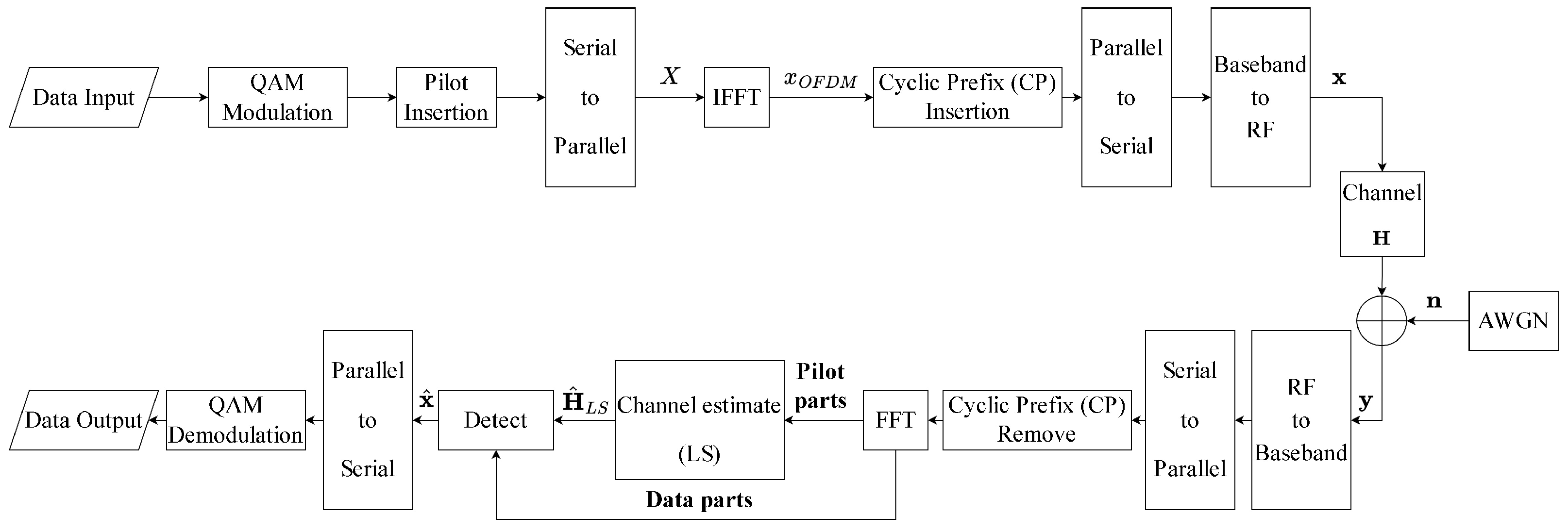
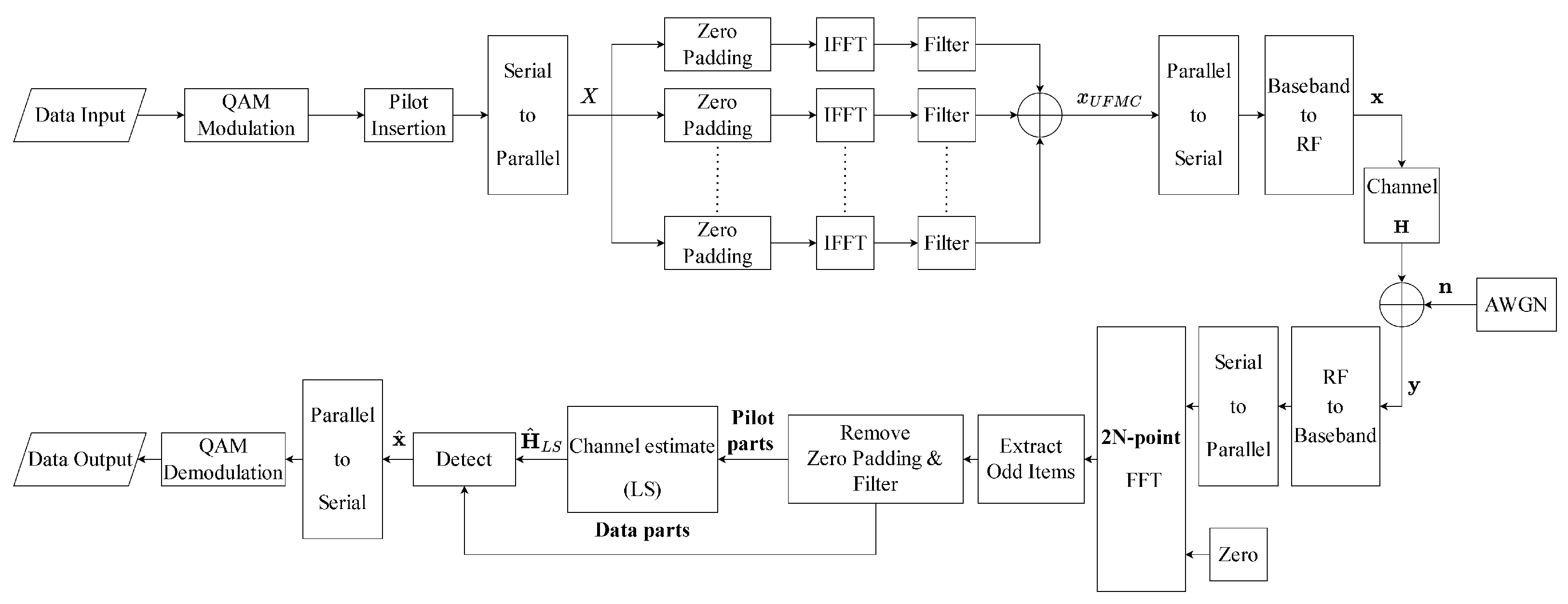
In this section, we follow the multi-user uplink M-MIMO environment illustrated in Section 2 to perform numerical simulations with OFDM and UFMC waveforms in order to evaluate and verify the performance of our proposed CHSOR receiver. The number of subcarriers of OFDM is set to be equal to the amount of data (512). In addition, it is necessary to add a CP with a length of 128, i.e., a quarter of the number of subcarriers, and 52 pilot data in one symbol. For UFMC, we set the number of subcarriers to 1024 and the total data volume to 512. This is divided into $B=16$ sub-bands, each with $M=32$ data. With these settings, 256 zeros must be padded at the head and the tail of the symbol to account for the difference between the number of subcarriers and the amount of data. 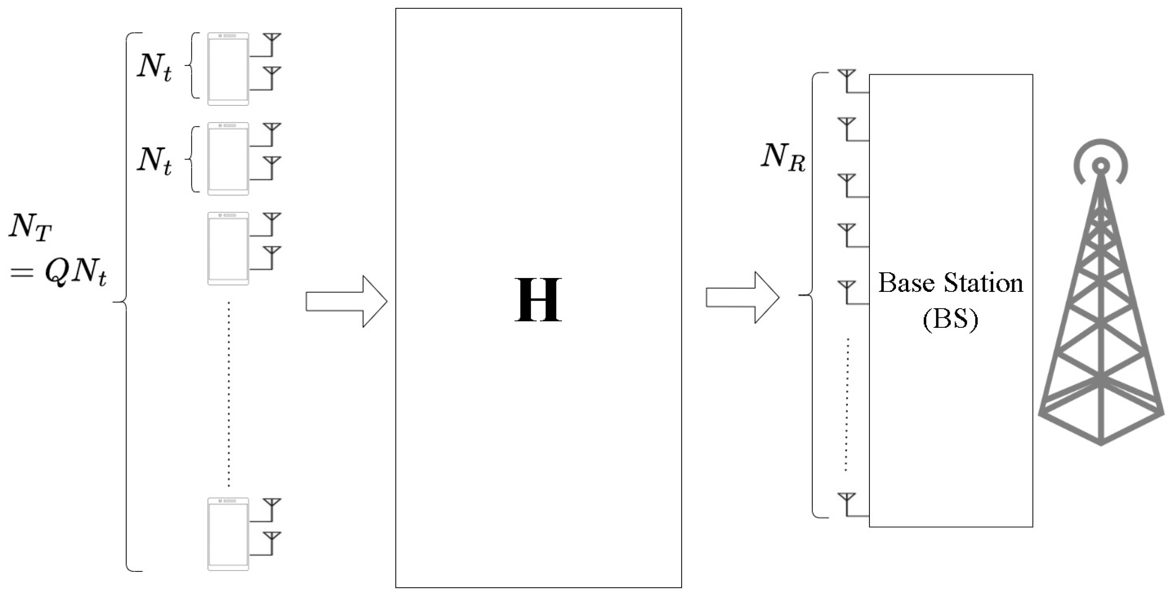For the filter type, we adopt a Chebyshev FIR filter [57,58] with a length of 43 and a side attenuation of 40 dB. To assess the impact of antenna configuration on performance, we set the number of transmit antennas $N_T$ to 16 and the number of receive antennas $N_R$ to 64, 128, 192, and 256. To facilitate further analysis, we used the parameter $\beta$ as the ratio of the receiving to transmitting antennas, or antenna ratio, denoted as $\beta ={\displaystyle \frac{N_R}{N_T}}$ [50,59]. In terms of channels, we established two flat Rayleigh fading channels with additive white Gaussian noise (AWGN). The maximum signal-to-noise ratio (SNR) for these channels was set at 50 dB and least-squares (LS) estimation was used to obtain the channel state information (CSI). For clarity, the above experimental parameters are tabulated in

Table 2. Parameters used in simulation scenarios.

Parameter	Value
Modulation	1024-QAM
Amount of data	512
Pilot Length	52
Number of transmitting antennas	16
Number of receiving antennas	64,128,192,256
Channel type	Rayleigh fading channel
Spatial-correlation coefficient (Tx, Rx)	(0.3, 0.4)
Noise	AWGN
Number of paths	2
The maximum SNR	50
Channel estimation	LS
Monte Carlo times	500,000
OFDM parameters
CP Length	128
UFMC parameters
Number of subcarriers	1024
Number of sub-bands	16
Number of subcarriers in each sub-band	32
Number of zero-padding	256
Filter type	Chebyshev FIR filter
Filter length	43
Filter sidelobe attenuation	40

.

The following experiments were applied to the OFDM and UFMC waveforms. Our proposed CHSOR scheme is compared with nine detectors, including SOR [17], MSOR [19], AOR [18], SSOR [20], SAOR [21], CSOR [22], Chebyshev-MAOR [27], Chebyshev-RI [26], and MMSE, with the MMSE scheme used as a benchmark. The MATLAB version R2022a mathematical software tool was used to simulate the numerical results and graphics. We executed 500,000 Monte Carlo rounds for each graph and used Microsoft Excel for the calculations and statistical tables.

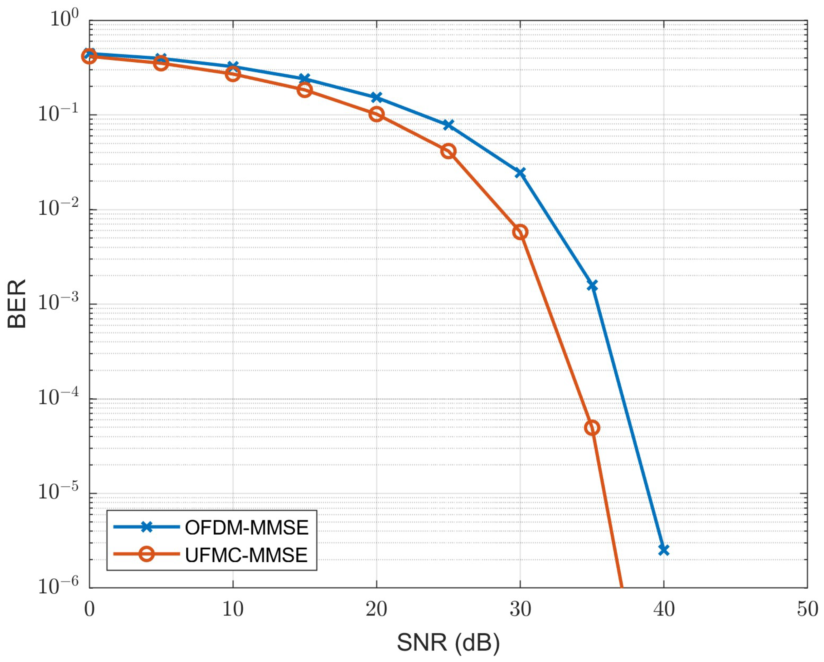
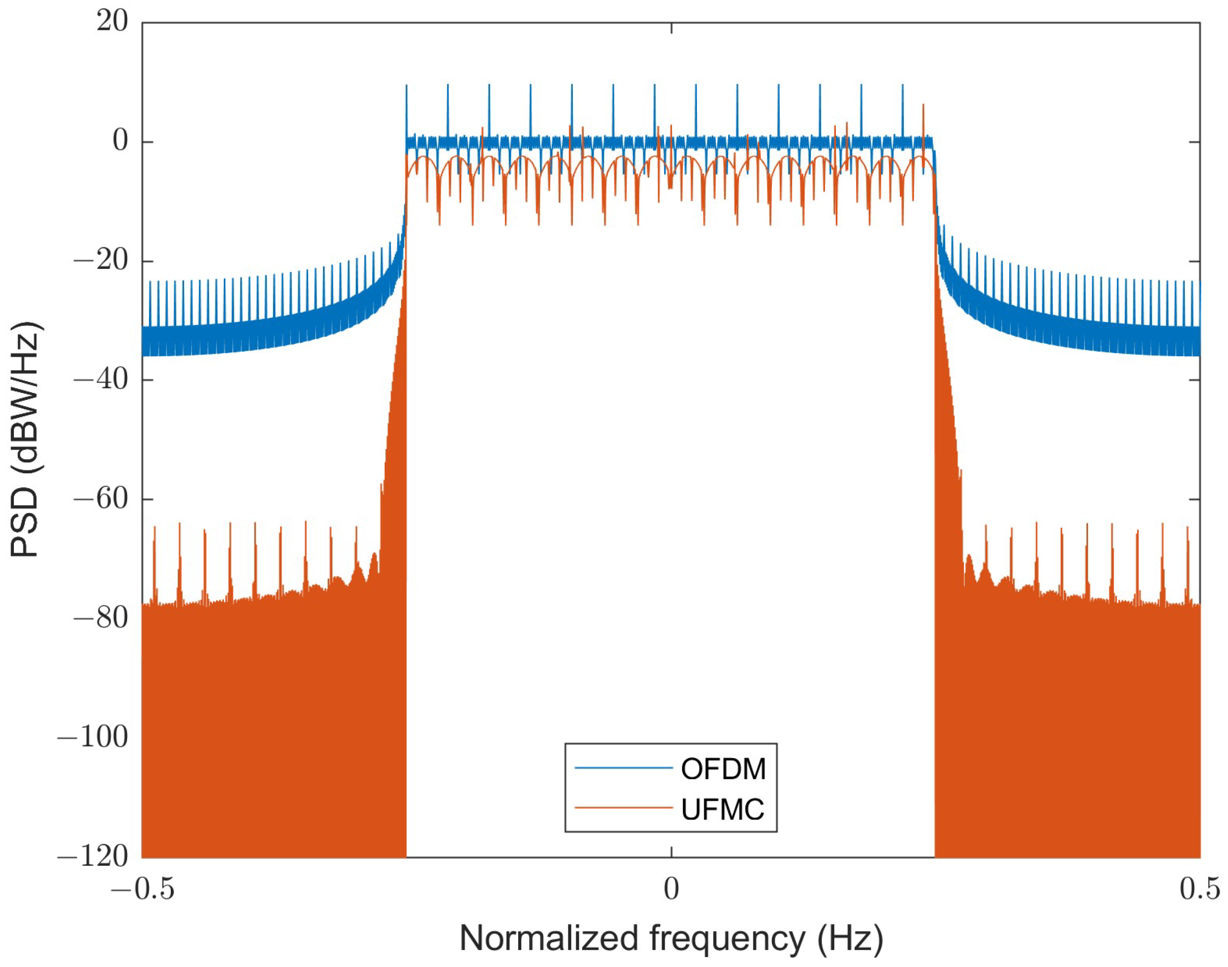
To observe which of UFMC and OFDM is more suitable for B5G and future communication environments, we used BER performance and power spectral density (PSD) indices to make an intuitive comparison. Figure 7 shows the BER vs. SNR for both waveforms detected using MMSE when $N_R\times N_T=64\times 16$. It can be seen that UFMC is better than OFDM; when the SNR is 35 dB, the BER of OFDM and UFMC are $1.599\times {10}^{-3}$ and $4.946\times {10}^{-5}$, respectively, which is a $96.907\%$ improvement. On the other hand, the PSD comparison in Figure 8 shows that the power sidelobe level of the OFDM waveform is larger than that of the UFMC waveform, indicating higher out-of-band emission and a tendency towards ACI. Therefore, we observe that the UFMC waveform has higher spectral efficiency and can better suppress the occurrence of ACI. In summary, the UFMC waveform is superior to the OFDM waveform regarding both BER performance and PSD, and is a promising B5G candidate waveform in future applications.

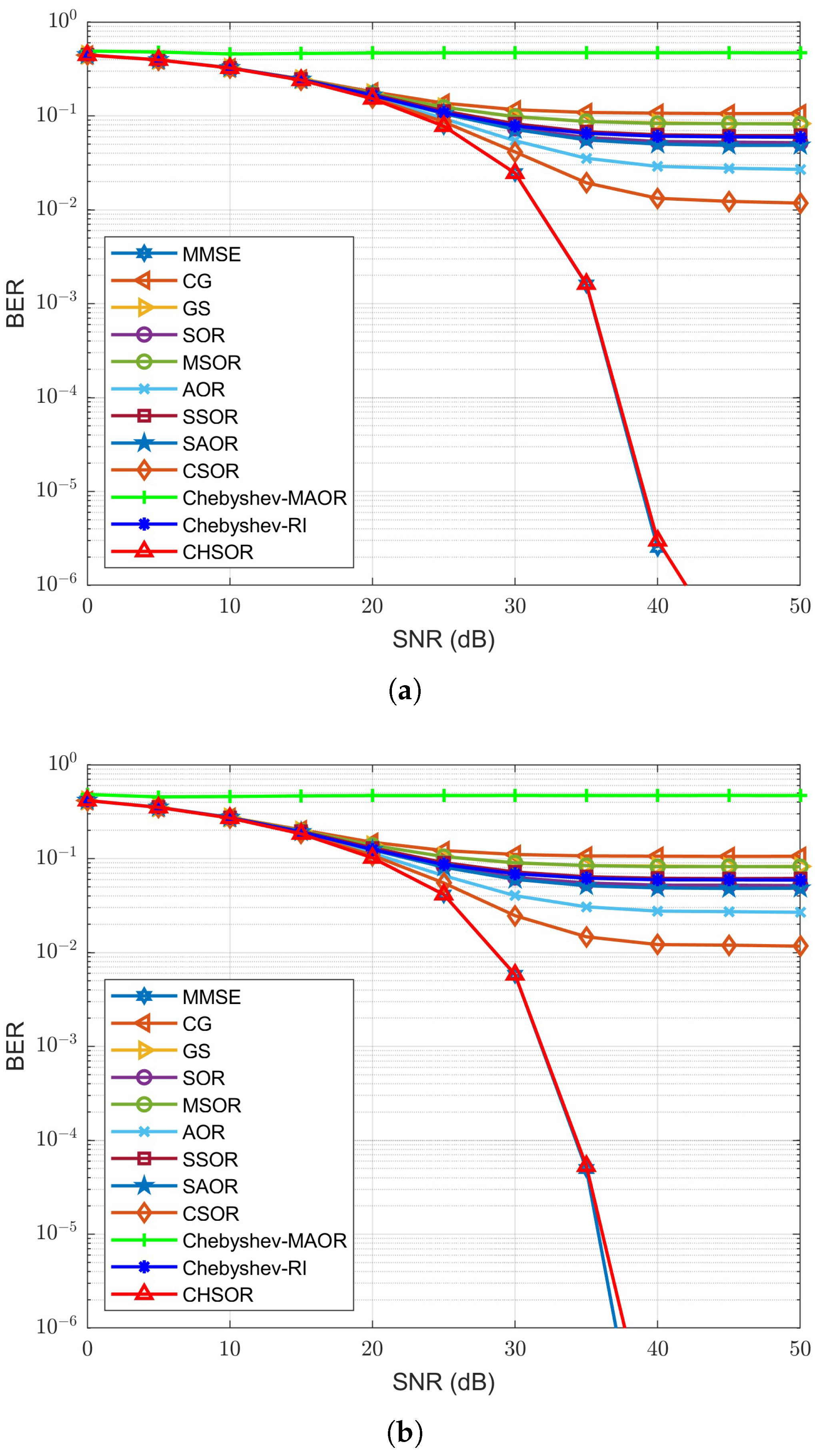
For BER performance, Figure 9, Figure 10, Figure 11 and Figure 12 show the BER vs. SNR curves of each method under different antenna configurations; Figure 9a, Figure 10a, Figure 11a and Figure 12a show the results for OFDM, while Figure 9b, Figure 10b, Figure 11b and Figure 12b show the results for UFMC. It is worth noting that the BER of the Gauss-Seidel (GS) and Conjugate-Gradient (CG) methods in Figure 9 and Figure 10 is relatively poor when the number of receive antennas $N_R$ is 64 and 128; thus, better performance at higher $N_R$ is unlikely. Based on these results, GS and CG are excluded from the subsequent figures for visual conciseness and to avoid clutter. 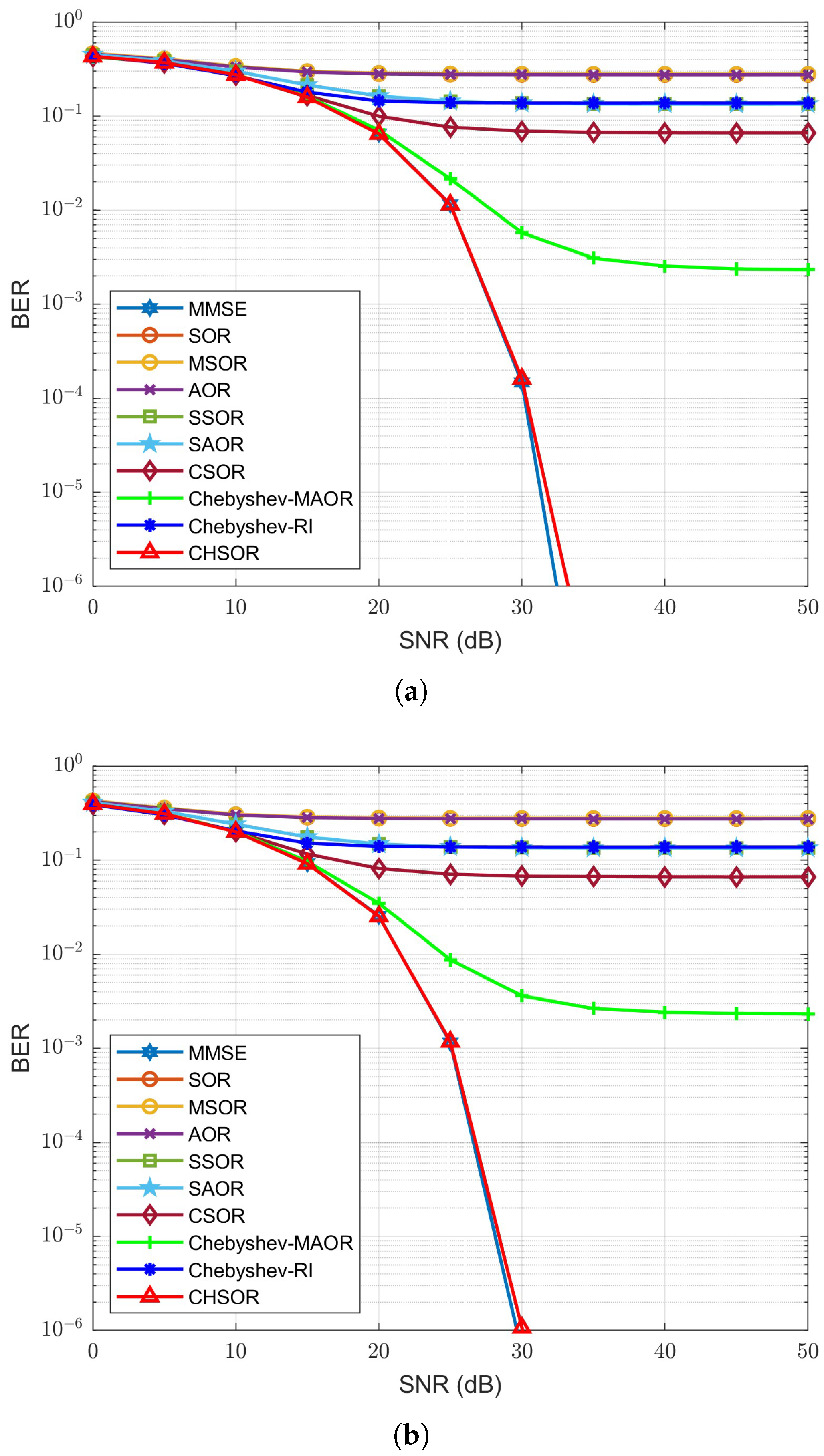On the other hand, Figure 9a,b shows that when $N_R\times N_T=64\times 16$ and the number of iterations is 4, the BER performance curves of the proposed CHSOR method almost overlap with the MMSE detector. In particular, in Figure 9a for the OFDM system, when the SNR is 35 dB, the BER numerical results of the proposed and CSOR methods are $1.620\times {10}^{-3}$ and $1.934\times {10}^{-2}$, respectively, which is an improvement of $91.624\%$. For the UFMC system in Figure 9b, the results show that the BER of the proposed and CSOR methods are $5.324\times {10}^{-5}$ and $1.469\times {10}^{-2}$, respectively, which is an improvement of $99.638\%$. Therefore, the proposed CHSOR detector provides a significant improvement compared to the CSOR method, especially for the UFMC system.

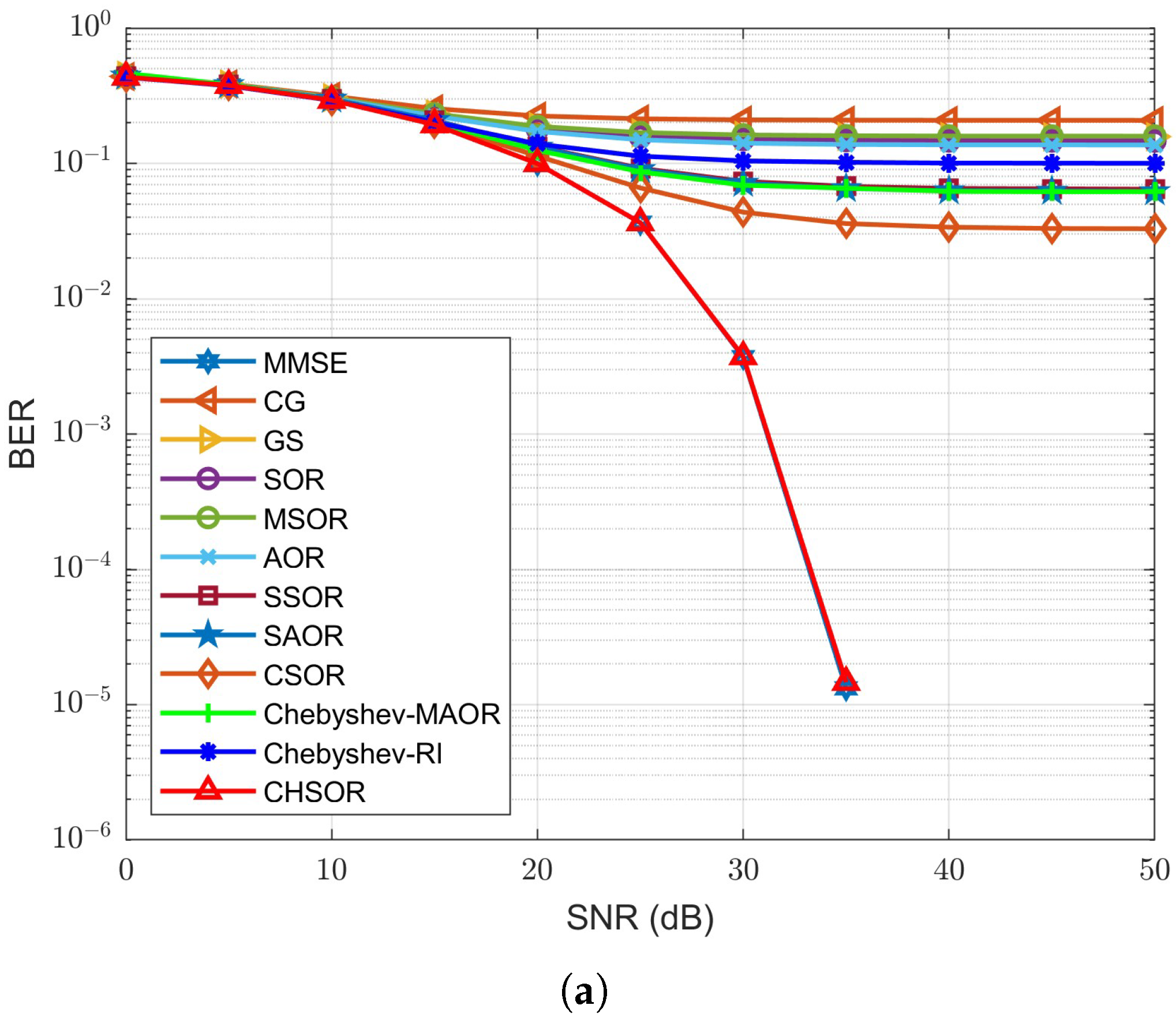
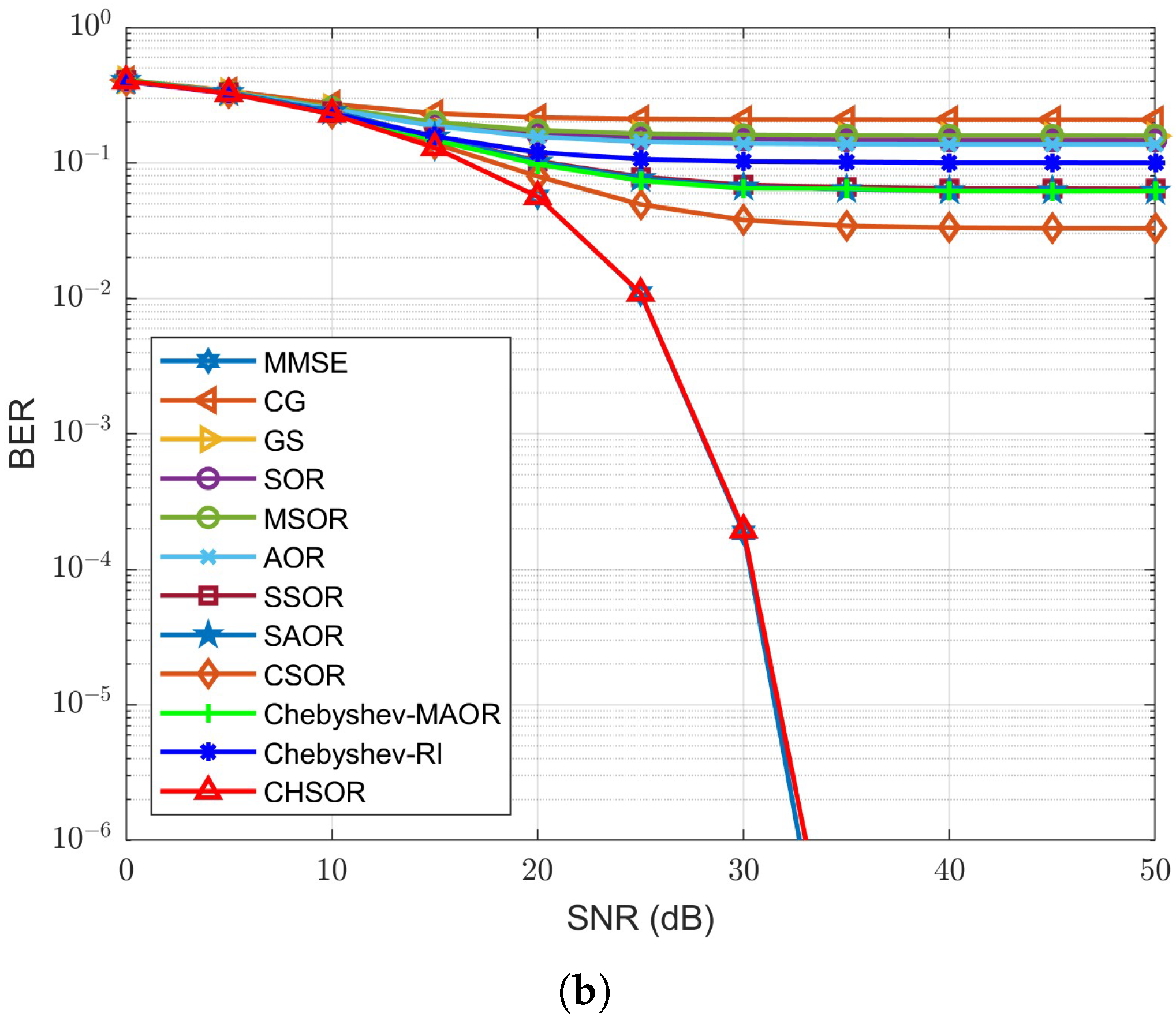
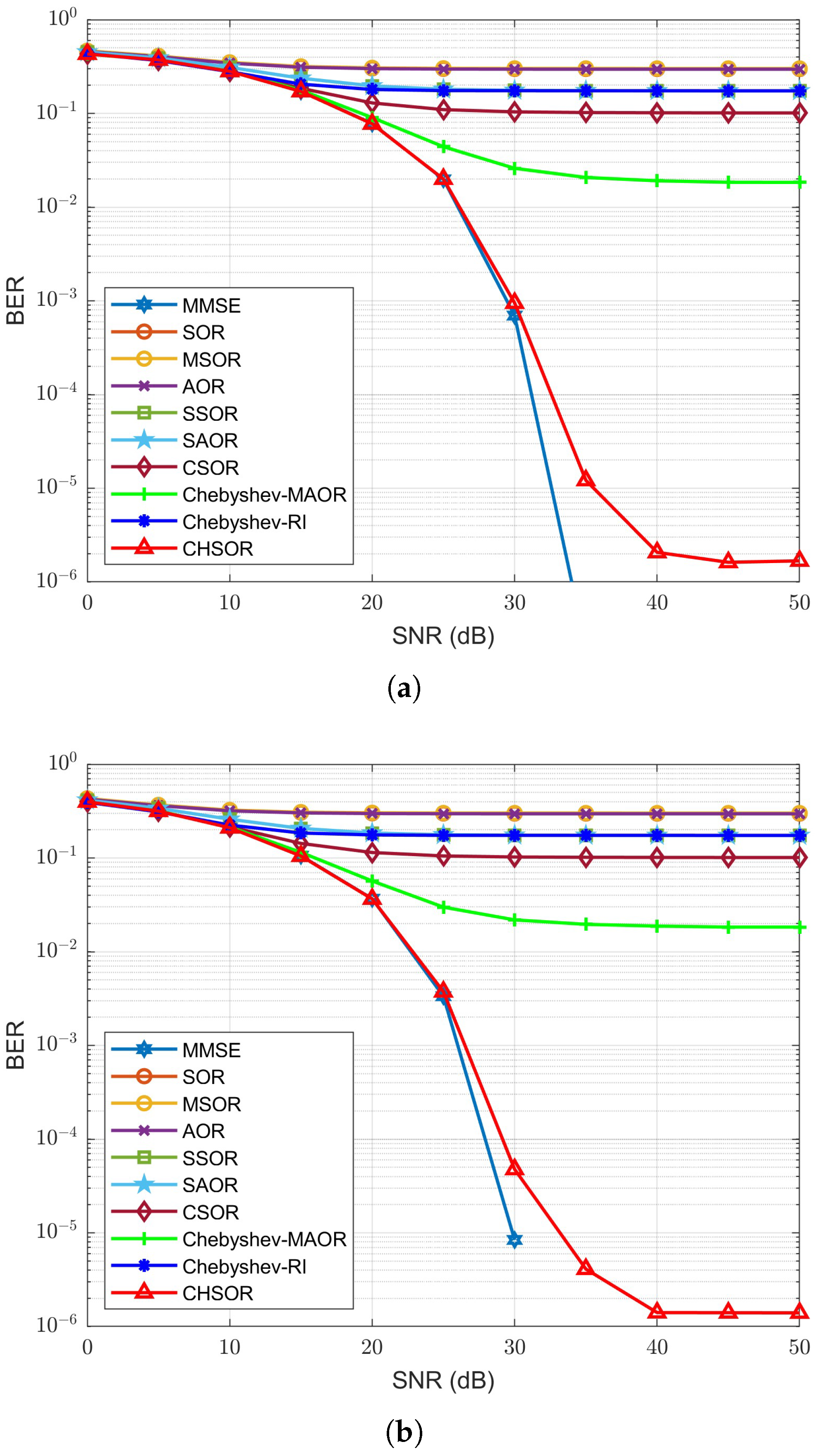
To observe the impact of M-MIMO on the BER performance of different detectors, we increased the number of receiving antennas from 128 to 192, and then to 256, as shown in Figure 10, Figure 11 and Figure 12, respectively. Our proposed CHSOR detector still provides superior BER performance compared to the others. It is worth mentioning that when the number of receiving antennas is 128, the BER performance curve of the proposed CHSOR method remains very close to the MMSE detection method after two iterations. When the number of antennas $N_R$ is increased to 192 and then again to 256, the BER performance of our proposed CHSOR method still maintains the same trend, only needing one iteration for both OFDM and UFMC. It can be seen that increasing the number of receiving antennas can speed up the convergence of the receiver without exception. These represent promising results for the application of M-MIMO to B5G applications.

For more clarity,

Table 3. BER numerical results improvement rate of proposed CHSOR and Chebyshev-MAOR at SNR = 30 dB for $N_R\times N_T=128\times 16$ and $N_R\times N_T=192\times 16$ under OFDM and UFMC.

	OFDM			UFMC
	CHSOR’s BER	Chebyshev-MAOR’s BER	Improvement Rate (%)	CHSOR’s BER	Chebyshev-MAOR’s BER	Improvement Rate (%)
$N_R$ = 128 $i=2$	$3.737\times {10}^{-3}$	$6.892\times {10}^{-2}$	94.578	$1.951\times {10}^{-4}$	$6.471\times {10}^{-2}$	99.699
$N_R$ = 192 $i=1$	$9.476\times {10}^{-4}$	$2.592\times {10}^{-2}$	96.344	$4.764\times {10}^{-5}$	$2.184\times {10}^{-2}$	99.782

enumerates the detailed BER results of the proposed CHSOR scheme and the Chebyshev-MAOR scheme. The improvement rate of the proposed CHSOR scheme is compared to the Chebyshev-MAOR scheme at SNR = 30 dB for $N_R\times N_T=128\times 16$ and $N_R\times N_T=192\times 16$ under both the OFDM and UFMC systems. Examining the numerical data in the CHSOR scheme in Table 3. when $N_R$ increases, in addition to the decrease in BER and enhancement of the improvement rate relative to other detectors, the application of UFMC for B5G systems is especially powerful.

According to the discussion in Section 3, convergence means that the signal vector gradually tends to a stable state after iteration; in other words, the BER reaches a stable value when the state no longer changes. To facilitate subsequent discussion, we define a convergence parameter that we call the BER altered rate ${\delta }^{\left(k\right)}$ for each iteration, as follows:

$${\delta }^{\left(k\right)}={\displaystyle \frac{{\psi }^{\left(k\right)}-{\psi }^{(k+1)}}{{\psi }^{\left(k\right)}}}$$

(41)

where ${\psi }^{\left(k\right)}$ represents the BER obtained at the $kth$ iteration and ${\delta }^{\left(k\right)}$ represents the altered rate in BER between the current iteration and the next iteration. In this paper, without loss of generality, we select a small enough ${\delta }^{\left(k\right)}$ variation of 1%; therefore, the iteration schemes can be convergent as long as they meet the following conditions:

$${\delta }^{\left(k\right)}<1\%.$$

(42)

To verify and compare the iteration convergence among all detectors in this study, we enumerate the BER altered rate for each iteration in

Table 4. The altered rate in BER between iterations of each method at $N_R\times N_T=64\times 16$ and $\mathrm{SNR}=37\mathrm{dB}$ for (a) OFDM and (b) UFMC.

Scheme	${\mathit{\delta }}^{\left(1\right)}$	${\mathit{\delta }}^{\left(2\right)}$	${\mathit{\delta }}^{\left(3\right)}$	${\mathit{\delta }}^{\left(4\right)}$	${\mathit{\delta }}^{\left(5\right)}$
(a)
SOR	31.973%	46.006%	60.562%	75.059%	83.093%
MSOR	27.944%	37.631%	50.730%	63.708%	74.285%
AOR	34.035%	53.444%	72.523%	86.377%	86.256%
SSOR	32.479%	41.178%	50.509%	58.834%	64.508%
SAOR	34.866%	44.787%	55.058%	64.132%	69.552%
CSOR	38.972%	60.083%	76.246%	85.268%	79.095%
Chebyshev-MAOR	−11.658%	−5.862%	−2.816%	−1.857%	−1.283%
Chebyshev-RI	25.154%	37.638%	54.286%	69.577%	81.921%
CHSOR	93.986%	93.033%	36.644%	2.966%	0.195%
(b)
MSOR	29.970%	37.830%	51.624%	66.313%	78.997%
AOR	34.100%	53.920%	74.763%	90.855%	96.159%
SSOR	32.565%	41.600%	51.857%	61.534%	68.615%
SAOR	34.970%	45.315%	56.784%	67.506%	74.740%
CSOR	39.202%	61.307%	79.396%	90.574%	93.302%
Chebyshev-MAOR	−11.660%	−5.846%	−2.813%	−1.854%	−1.280%
Chebyshev-RI	25.210%	37.957%	55.632%	74.093%	89.304%
CHSOR	95.928%	98.926%	93.233%	25.568%	0.894%

,

Table 5. The altered rate in BER between iterations of each method at $N_R\times N_T=128\times 16$ and $\mathrm{SNR}=34\mathrm{dB}$ for (a) OFDM and (b) UFMC.

Scheme	${\mathit{\delta }}^{\left(1\right)}$	${\mathit{\delta }}^{\left(2\right)}$	${\mathit{\delta }}^{\left(3\right)}$	${\mathit{\delta }}^{\left(4\right)}$	${\mathit{\delta }}^{\left(5\right)}$
(a)
SOR	54.855%	80.580%	95.354%	92.632%	34.096%
MSOR	51.649%	75.891%	92.787%	94.472%	55.665%
AOR	57.374%	85.023%	97.147%	87.003%	17.657%
SSOR	70.512%	89.219%	94.574%	79.240%	22.364%
SAOR	71.458%	90.276%	94.951%	75.746%	18.477%
CSOR	77.082%	95.770%	93.943%	32.539%	2.321%
Chebyshev-MAOR	45.546%	31.766%	23.355%	10.575%	5.714%
Chebyshev-RI	54.160%	79.458%	95.306%	88.386%	40.738%
CHSOR	97.426%	6.456%	−0.002%	0.035%	0.004%
(b)
SOR	55.083%	82.094%	97.525%	99.640%	91.201%
MSOR	51.844%	77.248%	95.202%	99.153%	98.063%
AOR	57.632%	86.603%	98.981%	99.737%	64.124%
SSOR	71.347%	91.470%	97.761%	98.461%	89.436%
SAOR	72.319%	92.552%	98.243%	98.691%	82.061%
CSOR	78.343%	97.640%	99.755%	91.586%	−1.653%
Chebyshev-MAOR	46.397%	31.882%	22.743%	10.002%	5.292%
Chebyshev-RI	54.522%	82.204%	98.437%	99.417%	85.085%
CHSOR	99.985%	28.235%	0%	−0.820%	0%

,

Table 6. The altered rate in BER between iterations of each method at $N_R\times N_T=192\times 16$ and $\mathrm{SNR}=32\mathrm{dB}$ for (a) OFDM and (b) UFMC.

Scheme	${\mathit{\delta }}^{\left(1\right)}$	${\mathit{\delta }}^{\left(2\right)}$	${\mathit{\delta }}^{\left(3\right)}$	${\mathit{\delta }}^{\left(4\right)}$	${\mathit{\delta }}^{\left(5\right)}$
(a)
SOR	68.751%	93.826%	97.939%	48.856%	3.412%
MSOR	66.646%	91.967%	97.924%	62.866%	5.643%
AOR	70.434%	95.359%	97.726%	35.321%	2.003%
SSOR	89.008%	98.134%	81.405%	11.401%	0.934%
SAOR	89.409%	98.240%	79.749%	10.561%	0.905%
CSOR	91.680%	98.491%	53.111%	3.244%	0.095%
Chebyshev-MAOR	92.071%	80.046%	43.541%	14.506%	7.654%
Chebyshev-RI	72.978%	95.883%	94.635%	39.338%	6.868%
CHSOR	59.505%	0.086%	−0.012%	−0.002%	0.002%
(b)
SOR	69.246%	95.436%	99.890%	96.420%	11.864%
MSOR	67.105%	93.680%	99.761%	98.853%	14.634%
AOR	70.964%	96.813%	99.950%	89.069%	4.630%
SSOR	90.438%	99.469%	99.658%	49.537%	2.752%
SAOR	90.905%	99.552%	99.618%	44.103%	3.670%
CSOR	93.238%	99.907%	97.484%	6.034%	3.670%
Chebyshev-MAOR	93.894%	80.776%	44.157%	16.235%	9.455%
Chebyshev-RI	74.083%	98.350%	99.848%	84.871%	11.382%
CHSOR	98.685%	−2.941%	0%	0%	0%

and

Table 7. The altered rate in BER between iterations of each method at $N_R\times N_T=256\times 16$ and $\mathrm{SNR}=30\mathrm{dB}$ for (a) OFDM and (b) UFMC.

Scheme	${\mathit{\delta }}^{\left(1\right)}$	${\mathit{\delta }}^{\left(2\right)}$	${\mathit{\delta }}^{\left(3\right)}$	${\mathit{\delta }}^{\left(4\right)}$	${\mathit{\delta }}^{\left(5\right)}$
(a)
SOR	77.258%	93.372%	89.753%	11.497%	0.633%
MSOR	75.907%	96.739%	91.871%	15.639%	0.897%
AOR	78.342%	97.875%	87.069%	8.460%	0.387%
SSOR	95.701%	96.458%	26.869%	2.027%	0.213%
SAOR	95.857%	96.373%	26.058%	2.006%	0.208%
CSOR	96.496%	92.876%	13.021%	0.575%	−0.031%
Chebyshev-MAOR	95.767%	38.911%	0.234%	0.380%	0.150%
Chebyshev-RI	85.245%	97.220%	70.412%	9.261%	1.720%
CHSOR	9.023%	−0.009%	0.007%	−0.001%	0%
(b)
SOR	78.108%	98.918%	99.868%	42.308%	1.111%
MSOR	76.737%	98.447%	99.885%	55.808%	3.794%
AOR	79.209%	99.258%	99.834%	28.911%	1.114%
SSOR	97.260%	99.928%	80.490%	5.080%	−0.282%
SAOR	97.410%	99.931%	78.588%	5.319%	0.281%
CSOR	98.171%	99.927%	46.047%	−1.437%	−0.850%
Chebyshev-MAOR	99.488%	96.588%	21.663%	0.279%	0.280%
Chebyshev-RI	87.531%	99.771%	98.085%	29.760%	7.368%
CHSOR	49.130%	−1.425%	0.281%	0%	0%

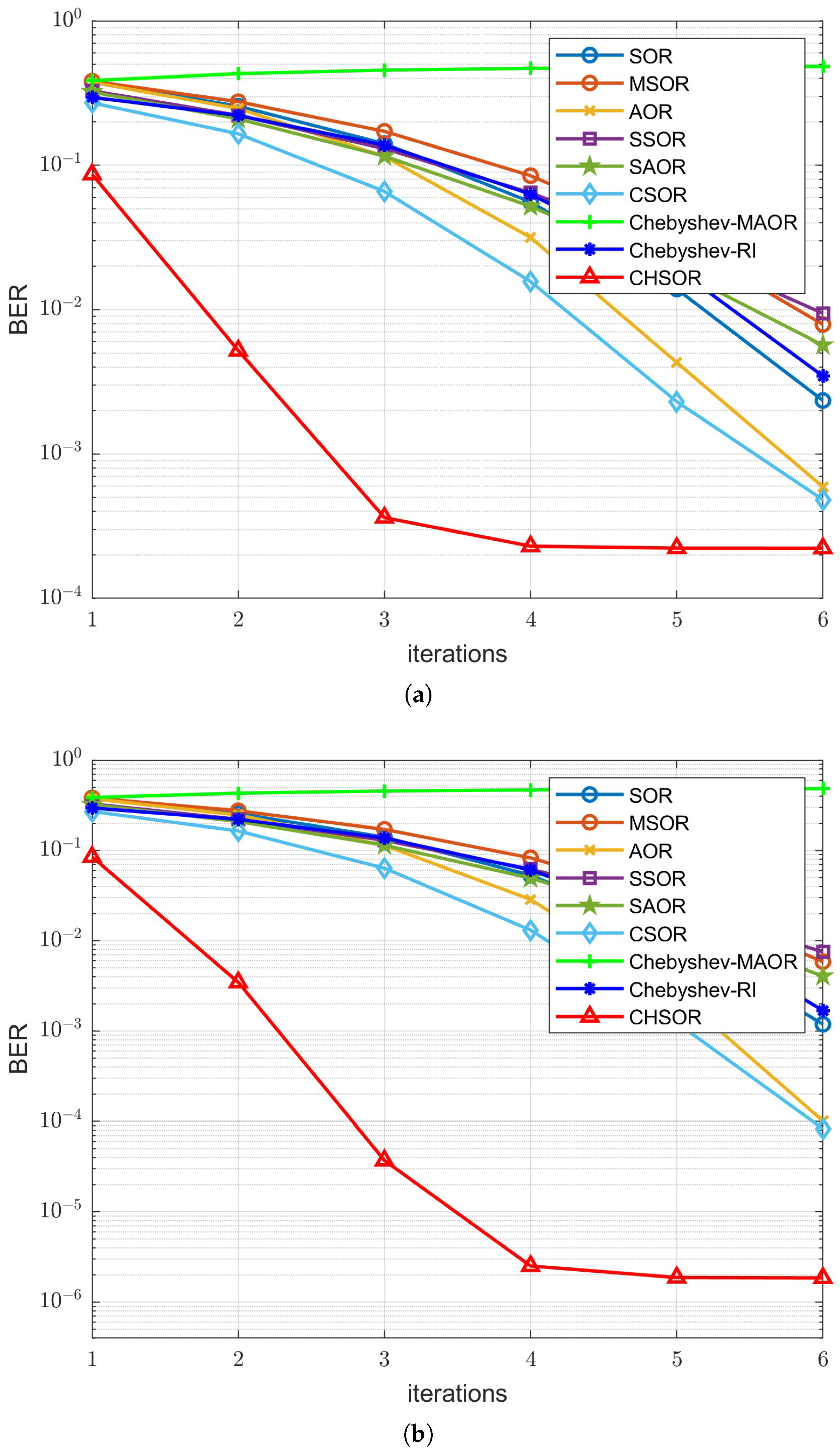
and plot the convergence curve in Figure 13, Figure 14, Figure 15 and Figure 16 with antenna configurations of $N_R\times N_T=64\times 16$, $N_R\times N_T=128\times 16$, $N_R\times N_T=192\times 16$, and $N_R\times N_T=256\times 16$, respectively. For Figure 13, the antenna configuration $N_R\times N_T$ is $64\times 16$ and the SNR is 37 dB, in which Figure 13a,b show the experiments conducted with the OFDM and UFMC systems, respectively. From the overall numerical analysis and observation of Table 4 and Figure 13a, it can be seen that the CHSOR method always performs the best and converges within five iterations. Compared to the second-best performing CSOR method, the BER improves by $90.329\%$. The results for the UFMC system are shown in Figure 13b. When the number of iterations is 5, the BER performance of the CHSOR method is improved by $99.849\%$ compared with the CSOR method. 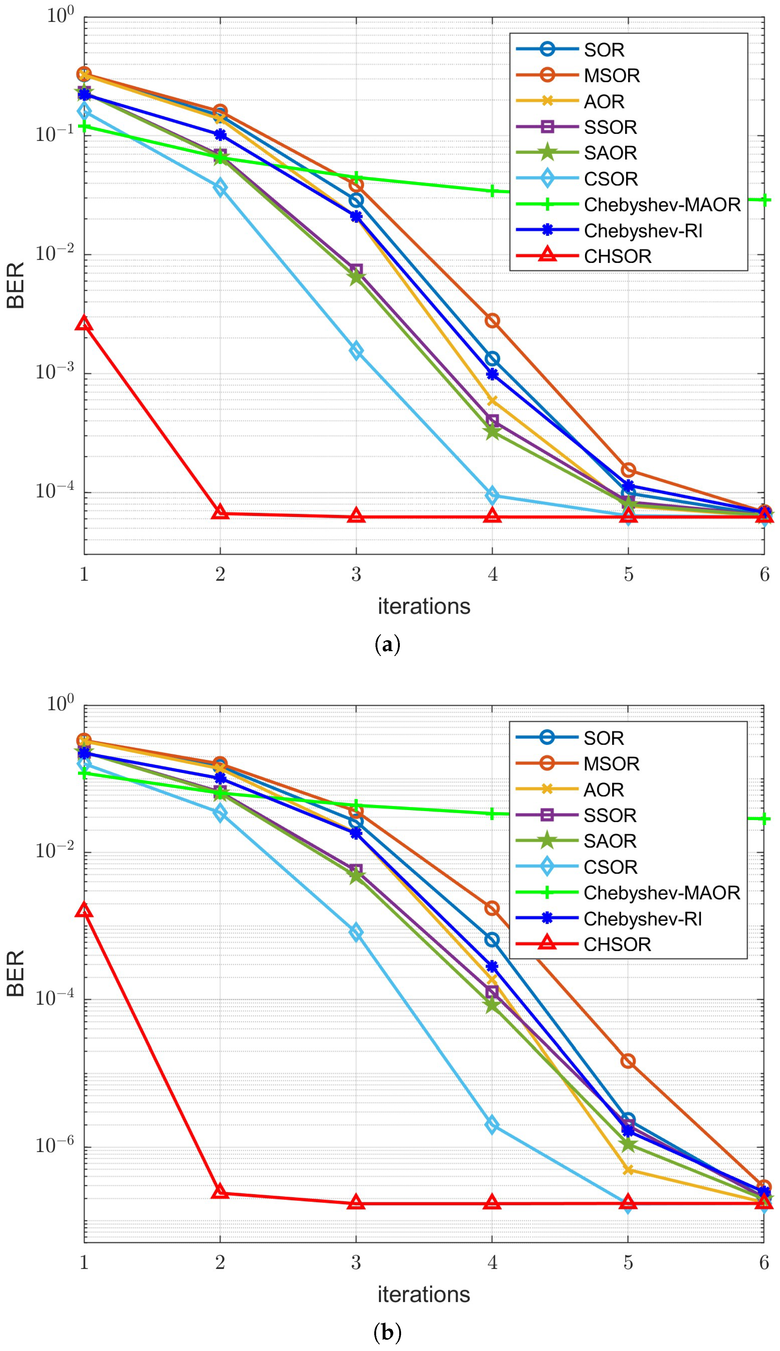When the $N_R$ is increased to 128 and the SNR is 34 dB, the proposed method converges in three iterations, while the other methods fail to converge even after five iterations. The simulation results for $N_R$ increased to 192 and SNR of 32 dB are shown in Figure 15a,b for the OFDM and UFMC systems, respectively. Similar to the results for $N_R$ of 128, Table 6b shows that the proposed method converges in three iterations for UFMC; furthermore, Table 6a shows that CHSOR converges after just two iterations for OFDM. 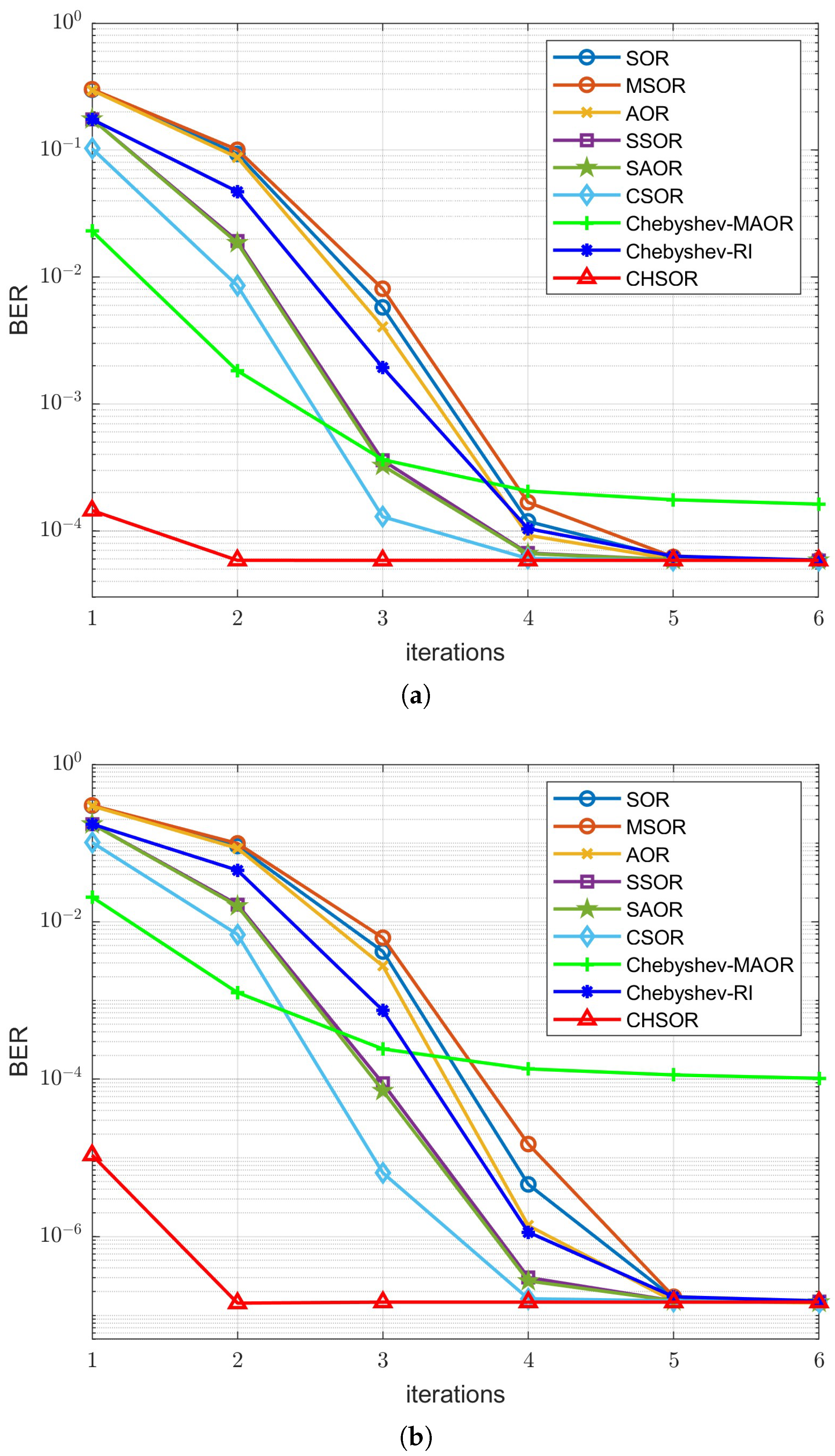When the number of iterations is 2, the proposed scheme has an improvement rate of $96.789\%$ and $99.989\%$ over Chebyshev-MAOR in the OFDM and UFMC systems, respectively. While CHSOR already demonstrates near-MMSE performance with only two iterations at $N_R$ of 192, its advantage becomes even better when the number of antennas is further increased to 256. As shown in the BER vs. iteration curves in Figure 16, the line for the CHSOR scheme is almost flat for both OFDM and UFMC systems, indicating that the proposed method converges almost within one iteration. With a large enough number of antennas, such as 192 or 256, it can significantly aid the HSOR stage to reduce the burden on the Chebyshev stage. In contrast, although Chebyshev-MAOR remains the fastest among the other methods, it still requires 3–4 iterations to reach a similar BER level, as evidenced in Table 7.

In summary, among the related detectors discussed in this paper, our proposed CHSOR algorithm has fast convergence speed and presents the best BER performance. Moreover, the experimental results in Figure 13, Figure 14, Figure 15 and Figure 16 and Table 4, Table 5, Table 6 and Table 7 along with Appendix A theoretically prove the convergence of the proposed scheme and verify convergence from the obtained experimental data.

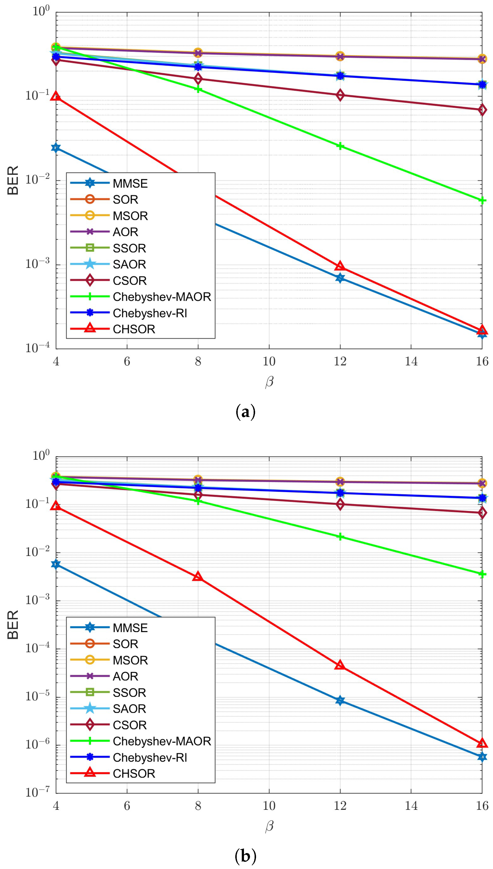
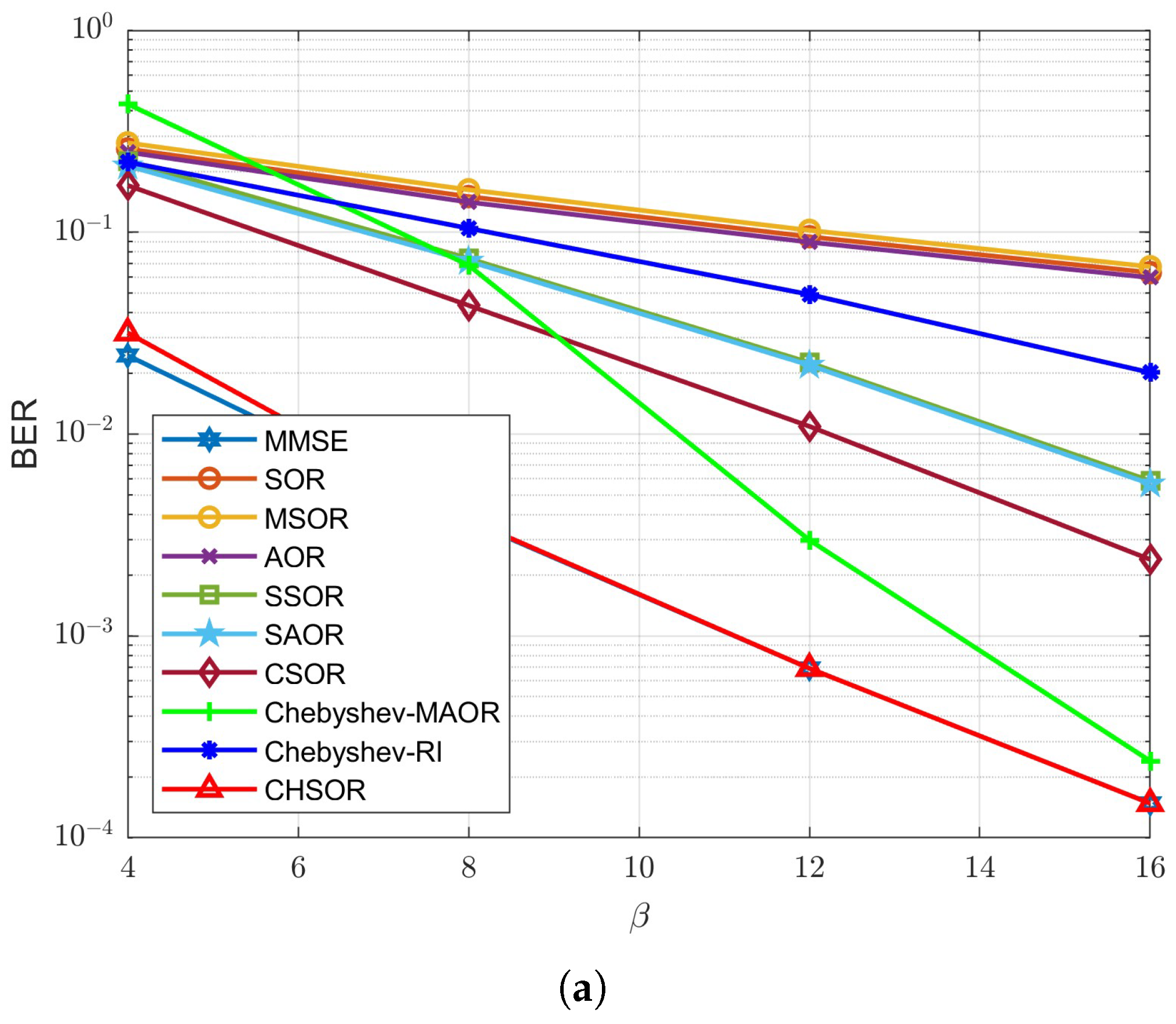
To analyze the BER performance of different detectors varies with different ratios of $N_R$ to the total number of user antennas $N_T$, we denote this as $\beta$, or the antenna ratio [50,59]. Figure 17 and Figure 18 show the results of the experiments with one and two iterations, respectively, when the SNR is 30 dB. In Figure 17, it can be seen tht when the antenna ratio is low, no method can achieve the BER performance of MMSE with one iteration. As $\beta$ increases, the BER of the proposed CHSOR scheme decreases significantly and gradually approaches the MMSE detector. Even though the BER of other methods also improves, the declining trend is quite slow compared with our CHSOR scheme. When $\beta$ is equal to 16, the CHSOR scheme is remarkably close to the MMSE detector. Next, the results with two iterations are shown in Figure 18. Compared with Figure 17, the BER performance of each method improves, but all are still inferior to our proposed method. Moreover, the curve of the CHSOR method almost coincides with the MMSE curve at any antenna ratio $\beta$.

To show the performance differences more intuitively, we enumerate the BER differences between each method and the MMSE detector under the same conditions in

Table 8. BER difference rate between the BER of all detection methods and MMSE at different $\beta$ when the number of iterations is 1 and the SNR is 30 dB for (a) OFDM and (b) UFMC.

Scheme	$\mathit{\beta }=4$	$\mathit{\beta }=8$	$\mathit{\beta }=12$	$\mathit{\beta }=16$
(a)
SOR	$3.533\times {10}^{-1}$	$3.242\times {10}^{-1}$	$2.982\times {10}^{-1}$	$2.778\times {10}^{-1}$
MSOR	$3.583\times {10}^{-1}$	$3.281\times {10}^{-1}$	$3.012\times {10}^{-1}$	$2.802\times {10}^{-1}$
AOR	$3.506\times {10}^{-1}$	$3.211\times {10}^{-1}$	$2.956\times {10}^{-1}$	$2.756\times {10}^{-1}$
SSOR	$3.047\times {10}^{-1}$	$2.291\times {10}^{-1}$	$1.753\times {10}^{-1}$	$1.374\times {10}^{-1}$
SAOR	$2.983\times {10}^{-1}$	$2.284\times {10}^{-1}$	$1.754\times {10}^{-1}$	$1.377\times {10}^{-1}$
CSOR	$2.473\times {10}^{-1}$	$1.582\times {10}^{-1}$	$1.032\times {10}^{-1}$	$6.916\times {10}^{-2}$
Chebyshev-MAOR	$3.621\times {10}^{-1}$	$1.181\times {10}^{-1}$	$2.506\times {10}^{-2}$	$5.661\times {10}^{-3}$
Chebyshev-RI	$2.713\times {10}^{-1}$	$2.196\times {10}^{-1}$	$1.740\times {10}^{-1}$	$1.381\times {10}^{-1}$
CHSOR	$7.368\times {10}^{-2}$	$4.886\times {10}^{-3}$	$2.463\times {10}^{-4}$	$1.453\times {10}^{-5}$
(b)
SOR	$3.719\times {10}^{-1}$	$3.276\times {10}^{-1}$	$2.986\times {10}^{-1}$	$2.776\times {10}^{-1}$
MSOR	$3.769\times {10}^{-1}$	$3.314\times {10}^{-1}$	$3.016\times {10}^{-1}$	$2.801\times {10}^{-1}$
AOR	$3.693\times {10}^{-1}$	$3.245\times {10}^{-1}$	$2.961\times {10}^{-1}$	$2.755\times {10}^{-1}$
SSOR	$3.232\times {10}^{-1}$	$2.319\times {10}^{-1}$	$1.747\times {10}^{-1}$	$1.360\times {10}^{-1}$
SAOR	$3.167\times {10}^{-1}$	$2.312\times {10}^{-1}$	$1.749\times {10}^{-1}$	$1.363\times {10}^{-1}$
CSOR	$2.656\times {10}^{-1}$	$1.608\times {10}^{-1}$	$1.025\times {10}^{-1}$	$6.779\times {10}^{-2}$
Chebyshev-MAOR	$3.810\times {10}^{-1}$	$1.195\times {10}^{-1}$	$2.164\times {10}^{-2}$	$3.637\times {10}^{-3}$
Chebyshev-RI	$2.898\times {10}^{-1}$	$2.230\times {10}^{-1}$	$1.745\times {10}^{-1}$	$1.381\times {10}^{-1}$
CHSOR	$8.548\times {10}^{-2}$	$2.900\times {10}^{-3}$	$3.604\times {10}^{-5}$	$4.883\times {10}^{-7}$

and

Table 9. BER difference rate between the BER of all detection methods and MMSE at different $\beta$ when the number of iterations is 2 and the SNR is 30 dB for (a) OFDM and (b) UFMC.

Scheme	$\mathit{\beta }=4$	$\mathit{\beta }=8$	$\mathit{\beta }=12$	$\mathit{\beta }=16$
(a)
SOR	$2.342\times {10}^{-1}$	$1.465\times {10}^{-1}$	$9.432\times {10}^{-2}$	$6.295\times {10}^{-2}$
MSOR	$2.526\times {10}^{-1}$	$1.586\times {10}^{-1}$	$1.015\times {10}^{-1}$	$6.732\times {10}^{-2}$
AOR	$2.248\times {10}^{-1}$	$1.372\times {10}^{-1}$	$8.861\times {10}^{-2}$	$5.942\times {10}^{-2}$
SSOR	$2.002\times {10}^{-1}$	$7.042\times {10}^{-2}$	$2.190\times {10}^{-2}$	$5.719\times {10}^{-3}$
SAOR	$1.886\times {10}^{-1}$	$6.819\times {10}^{-2}$	$2.126\times {10}^{-2}$	$5.519\times {10}^{-3}$
CSOR	$1.461\times {10}^{-1}$	$3.969\times {10}^{-2}$	$1.023\times {10}^{-2}$	$2.243\times {10}^{-3}$
Chebyshev-MAOR	$4.071\times {10}^{-1}$	$6.498\times {10}^{-2}$	$2.293\times {10}^{-3}$	$9.210\times {10}^{-5}$
Chebyshev-RI	$1.981\times {10}^{-1}$	$1.009\times {10}^{-1}$	$4.847\times {10}^{-2}$	$2.002\times {10}^{-2}$
CHSOR	$7.230\times {10}^{-3}$	$4.010\times {10}^{-5}$	$6.793\times {10}^{-9}$	$-8.832\times {10}^{-8}$
(b)
SOR	$2.521\times {10}^{-1}$	$1.480\times {10}^{-1}$	$9.257\times {10}^{-2}$	$6.061\times {10}^{-2}$
MSOR	$2.708\times {10}^{-1}$	$1.604\times {10}^{-1}$	$9.991\times {10}^{-2}$	$6.501\times {10}^{-2}$
AOR	$2.425\times {10}^{-1}$	$1.385\times {10}^{-1}$	$8.672\times {10}^{-2}$	$5.707\times {10}^{-2}$
SSOR	$2.174\times {10}^{-1}$	$6.899\times {10}^{-2}$	$1.803\times {10}^{-2}$	$3.672\times {10}^{-3}$
SAOR	$2.055\times {10}^{-1}$	$6.662\times {10}^{-2}$	$1.733\times {10}^{-2}$	$3.479\times {10}^{-3}$
CSOR	$1.618\times {10}^{-1}$	$3.741\times {10}^{-2}$	$7.688\times {10}^{-3}$	$1.206\times {10}^{-3}$
Chebyshev-MAOR	$4.261\times {10}^{-1}$	$6.420\times {10}^{-2}$	$1.323\times {10}^{-3}$	$1.610\times {10}^{-5}$
Chebyshev-RI	$2.160\times {10}^{-1}$	$1.023\times {10}^{-1}$	$4.607\times {10}^{-2}$	$1.697\times {10}^{-2}$
CHSOR	$7.884\times {10}^{-3}$	$8.138\times {10}^{-6}$	$6.836\times {10}^{-8}$	$4.185\times {10}^{-9}$

based on Figure 17 and Figure 18. Table 8a for the OFDM system shows that when $\beta$ is 12 and 16, the distances are $2.463\times {10}^{-4}$ and $1.453\times {10}^{-5}$, respectively. Table 8b for the UFMC system shows that when $\beta$ is 12 and 16, the gap can be reduced to $3.604\times {10}^{-5}$ and $4.883\times {10}^{-7}$, respectively. Moreover, when the number of iterations is 2 and with a sufficiently high $\beta$, the gap between our method and MMSE can be reduced to approximately order ${10}^{-9}$ for both the OFDM or UFMC systems, as enumerated in Table 9.

Thus far, the discussion on the impact of the number of receive antennas and antenna ratios on the uplink receiver of the BER performance has been well established. Due to the advantage actuated by the spatial diversity gain of massive antennas, as long as the antenna ratio $\beta$ becomes higher, the BER of any method will decrease without exception. It is worth noting that the effect is particularly significant for our proposed CHSOR scheme. Moreover, this performance echoes what was inferred earlier; when $N_R$ increases, BER performance can be improved and convergence acceleration can be achieved with reduced complexity. This means that the experimental results are reasonable and confirms that the proposed method can adequately and efficiently utilize the spatial diversity gain, resulting in performance quite close to that of the MMSE baseline. Moreover, the sensitivity of different schemes to the number of antennas is also worth observing and discussing. For instance, Chebyshev-MAOR exhibits strong dependence on the number of antennas. Its performance degrades considerably under low antenna ratio MIMO configurations, such as $\beta =4$, and only shows good results when the number of receiving antennas is high enough, such as $\beta =16$. On the other hand, for Chebyshev-RI the performance improvement remains marginal even when the number of antennas increases. In contrast, the proposed CHSOR method demonstrates robust and consistent performance across various antenna settings. CHSOR remains stable and effective regardless of whether the antenna ratio is low or high, highlighting its superior adaptability and reliability in M-MIMO systems.

4.2. Computational Complexity Analysis

4.2.1. Complexity Formula Analysis

In this subsection, we evaluate the computational complexity of the proposed method in terms of the number of required complex multiplications and additions (CMAs) and compare it with other detection methods mentioned in this paper [17,18,19,20,21,22,24,25]. We use i and $N_T$ to denote the number of iterations and total number of user antennas, respectively. We sequentially analyze the algebraic calculation of the proposed CHSOR detection method through its iterative equation as follows:

$$\begin{array}{c}\hfill {\tilde{\mathbf{x}}}^{\left(k\right)}={\displaystyle \frac{2{\mu }^{\left(k\right)}}{{\mu }^{(k-1)}·\mu }}({\mathbf{G}}_{HSOR}{\tilde{\mathbf{x}}}^{(k-1)}+{\mathbf{d}}_{HSOR})-{\displaystyle \frac{{\mu }^{\left(k\right)}}{{\mu }^{(k-2)}}}{\tilde{\mathbf{x}}}^{(k-2)}\end{array}$$

(43)

where the iteration matrix ${\mathbf{G}}_{HSOR}$ is equal to $\left[{\mathbf{M}}_{SOR}^{-1}{\mathbf{N}}_{SOR}{\mathbf{M}}_{MSOR}^{-1}{\mathbf{N}}_{MSOR}\right]$, which requires $\left[6N_T^2-2N_T\right]$ CMAs, and the compensation vector ${\mathbf{d}}_{HSOR}$ is $\left[{\mathbf{G}}_{SOR}{\mathbf{d}}_{MSOR}+{\mathbf{d}}_{SOR}\right]$, which needs $\left[3N_T^2+N_T\right]$ CMAs. Therefore, according to Equation (38), the operation complexity for the first stage can be obtained as a total of $\left[11N_T^2-N_T\right]$ CMAs. For the second stage, executing the Chebyshev acceleration algorithm, including $\left[{\displaystyle \frac{2{\mu }^{\left(k\right)}}{{\mu }^{(k-1)}·\mu }}({\mathbf{G}}_{HSOR}{\tilde{\mathbf{x}}}^{(k-1)}+{\mathbf{d}}_{HSOR})\right]$, $\left[-{\displaystyle \frac{{\mu }^{\left(k\right)}}{{\mu }^{(k-2)}}}{\tilde{\mathbf{x}}}^{(k-2)}\right]$, and their addition operation, requires $\left[2N_T^2+N_T\right]$, $N_T$, and $N_T$ CMAs, respectively. Because the second stage is an iterative algorithm, the above computational complexity is added and multiplied by the number of iterations i, expressed as $\left[i(2N_T^2+3N_T)\right]$. Therefore, our proposed CHSOR method requires a total of $\left[11N_T^2-N_T+i(2N_T^2+3N_T)\right]$ CMAs. The complexity analysis for the other methods is derived similarly and is not elaborated here. For greater clarity, the algebraic expressions of the computational complexity for different schemes are tabulated in

Table 10. Algebraic expressions of computational complexity for different detectors.

Detection Methods	Complex Multiplications and Additions (CMAs)
SOR	${\displaystyle \frac{5}{2}}{N}_T^2+{\displaystyle \frac{1}{2}}{N}_T+i(2N_T^2+N_T)$
MSOR	${\displaystyle \frac{5}{2}}{N}_T^2-{\displaystyle \frac{3}{2}}{N}_T+i(2N_T^2+N_T)$
AOR	$3N_T^2+i\left(3N_T^2\right)$
SSOR	$5N_T^2+N_T+i(4N_T^2+2N_T)$
SAOR	$6N_T^2+i\left(6N_T^2\right)$
CSOR	${\displaystyle \frac{5}{2}}{N}_T^2+{\displaystyle \frac{1}{2}}{N}_T+i(2N_T^2+3N_T)$
Chebyshev-MAOR	${\displaystyle \frac{17}{2}}{N}_T^2-{\displaystyle \frac{3}{2}}{N}_T+i(2N_T^2+3N_T)$
Chebyshev-RI	$3N_T^2-2N_T+i(2N_T^2+3N_T)$
CHSOR	$11N_T^2-N_T+i(2N_T^2+3N_T)$

. It is worth mentioning that it can be seen from the algebraic formulas in Table 10 that the complexity is independent of the number of receiving antennas. Of course, this is an important attraction for the B5G uplink system, which urgently needs M-MIMO.

4.2.2. Complexity Quantitative Analysis

For more intuitive comparison and quantitative analysis, the exact parameter values are substituted in Table 10, with numerical values enumerated in

Table 11. Numerical complexity comparison for different detectors with $N_T=16$.

Detection Methods	CMAs $\mathit{i}=1$	CMAs $\mathit{i}=2$	CMAs $\mathit{i}=3$	CMAs $\mathit{i}=4$	CMAs $\mathit{i}=5$	CMAs $\mathit{i}=6$
SOR	1176	1704	2232	2760	3288	3816
MSOR	1144	1672	2200	2728	3256	3784
AOR	1536	2304	3072	3840	4608	5376
SSOR	2352	3408	4464	5520	6576	7632
SAOR	3072	4608	6144	7680	9216	10,752
CSOR	1464	2280	3096	3912	4728	5544
Chebyshev-MAOR	2968	3784	4600	5416	6232	7048
Chebyshev-RI	1552	2368	3184	4000	4816	5632
CHSOR	3360	3920	4480	5040	5600	6160

and presented using a bar chart in Figure 19.

Next, computational complexity and BER performance are discussed to provide a comprehensive comparison. It can be seen from Figure 9a,b that with four iterations the proposed method improves the BER by $91.624\%$ and $99.638\%$ compared with CSOR in the OFDM and UFMC systems, respectively. For complexity, Table 11 shows that it only increases by $22.381\%$ regardless of whether the OFDM or UFMC system is used.

Moreover, Figure 13 along with Table 4 and Table 11 allow us to observe and compare each method’s iterative procedure and required complexity when it reaches convergence under the antenna configuration with $N_R\times N_T=64\times 16$ and SNR at 37 dB. Evidently, the CHSOR method converges at the fourth iteration and the complexity load is 5040 CMAs. Among the other methods, the CSOR scheme has the best performance; however, it still has not converged after six iterations, and its complexity burden of 5544 CMAs has exceeded that of the CHSOR method after four iterations. Although at first glance our proposed CHSOR scheme seems slightly higher than the CSOR method with the same number of iterations, the BER performance of the CHSOR scheme can be much better than that of the CSOR method with only a few iterations.

As previously mentioned, Figure 13, Figure 14, Figure 15 and Figure 16 show the relationship between the number of iterations i and BER performance among all schemes for different antenna configurations. From these results, we can conclude that faster the convergence is achieved when there are more antennas at the receiving end. Taking the proposed method as an example, when $N_R$ increases from 64 to 256, the number of iterations required for convergence can be reduced from 4 to 2 or even 1; in addition, the BER performance is significantly better than other methods. Therefore, the proposed CHSOR detector achieves a strong balance between computational complexity and BER performance. When $N_R$ increases, the proposed CHSOR detector takes full advantage of the spatial diversity gain of M-MIMO and the optimal initial conditions of the HSOR stage to provide excellent convergence speed without sacrificing any computational complexity, thereby considering both computational complexity and BER performance.

5. Conclusions

In development to date, M-MIMO has become the hope for the next generation of advanced wireless communications. In this article, we propose a high-efficiency and low-complexity two-stage receiver called CHSOR to overcome the challenge of M-MIMO technology applied to B5G uplink environments.

First, we utilize the double refinement feature of SOR and MSOR to provide more accurate initial status and estimated parameters for the next stage. In the second stage, the Chebyshev recurrence relation is used to achieve rapid convergence and higher BER performance estimation. As expected, the first stage facilitates the speed and convergence direction of the second stage.

Our simulation results show that the proposed CHSOR scheme has the best BER performance compared to previous detectors. In particular, it delivers a 91.624% BER improvement over CSOR, demonstrating superior detection capability. Moreover, thanks to its rapid convergence, the proposed CHSOR scheme does not need to sacrifice complexity for BER performance. At the same time, its computational complexity is independent of the number of receiving antennas; as the antenna ratio increases, not only does its BER performance improve, its complexity decreases instead of increasing, since convergence is accelerated. This is undoubtedly an important benefit for the B5G uplink system, which urgently needs M-MIMO. It is worth mentioning that as the antenna ratio continues to increase, the proposed CHSOR scheme converges to the optimal MMSE baseline in almost one iteration; therefore, we expect that the load of the Chebyshev stage can be significantly reduced.

In summary, the proposed method uses a double refinement feature and a relatively simple SOR-based architecture. This results in excellent characteristics of high BER performance and moderate computational complexity that make it suitable for application in current and next-generation wireless communication environments and provides a high-performance option with guaranteed convergence for B5G uplink systems.