LLM-Based Cyberattack Detection Using Network Flow Statistics

Abstract

Cybersecurity is a growing area of research due to the constantly emerging new types of cyberthreats. Tools and techniques exist to keep systems secure against certain known types of cyberattacks, but are insufficient for others that have recently appeared. Therefore, research is needed to design new strategies to deal with new types of cyberattacks as they arise. Existing tools that harness artificial intelligence techniques mainly use artificial neural networks designed from scratch. In this paper, we present a novel approach for cyberattack detection using an encoder–decoder pre-trained Large Language Model (T5), fine-tuned to adapt its classification scheme for the detection of cyberattacks. Our system is anomaly-based and takes statistics of already finished network flows as input. This work makes significant contributions by introducing a novel methodology for adapting its original task from natural language processing to cybersecurity, achieved by transforming numerical network flow features into a unique abstract artificial language for the model input. We validated the robustness of our detection system across three datasets using undersampling. Our model achieved consistently high performance across all evaluated datasets. Specifically, for the CIC-IDS-2017 dataset, we obtained an accuracy, precision, recall, and F-score of more than 99.94%. For CSE-CIC-IDS-2018, these metrics exceeded 99.84%, and for BCCC-CIC-IDS-2017, they were all above 99.90%. These results collectively demonstrate superior performance for cyberattack detection, while maintaining highly competitive false-positive rates and false-negative rates. This efficacy is achieved by relying exclusively on real-world network flow statistics, without the need for synthetic data generation.

1. Introduction

Cybersecurity has become an essential field due to the continuous emergence of new risks. Given the wide range of threats that can affect a computer system, it is crucial to implement techniques and tools to minimize the impact of persistent attacks on computer networks. However, such measures are still insufficient, as cybercriminals are always ahead of the curve, constantly developing new types of cyberthreats [1].

It is thus necessary to protect information since it is the most important asset of an organization. To this end, we have a wide range of tools at our disposal that can be used to reduce the risks faced by these systems.

In terms of protecting organization networks, we have so-called Security Information and Event Management (SIEM) systems [2], Intrusion Prevention Systems (IPSs) [3], and Intrusion Detection Systems (IDSs) [4].

An IDS can be classified into host-based and network-based. The first monitors a computer, and the second, known as the Network Intrusion Detection System (NIDS), monitors a network. Finally, a NIDS could be classified as (a) signature-based, focused on signatures of attacks or specific patterns; or (b) anomaly-based, which is focused on abnormalities and malicious activity, identifying departures from the normal behavior of computer networks [5]. It is worth noting that our approach is aligned with anomaly-based NIDS.

The main purpose of the aforementioned tools is the detection of cyberattacks. However, the continuous appearance of new types of attacks makes it necessary to have cyberattack detection systems that can use Artificial Intelligence (AI) techniques to infer new attacks. To develop such systems, Deep Learning (DL) [6] algorithms can be used and, more specifically, a model based on Artificial Neural Networks (ANNs) [7].

This task can be solved by defining and training a model from scratch, or by selecting an existing pre-trained one, to apply fine-tuning or transfer learning, which, despite being similar techniques, have certain differences. The use of pre-trained models is growing, particularly for building new ones, typically aimed at solving specific tasks related to the original one. This approach is widely used in supervised learning for models based on different tasks, such as face recognition, object recognition, and Natural Language Processing (NLP) [8].

Transfer learning [9] is a well-established technique focused on modifying part of the architecture of an existing ANN that has already been trained, replacing the last layers with new ones that are relevant to the new task, and then retraining only the altered layers to adapt a model to a new domain.

In contrast, fine-tuning [10] is an approach used to modify weights of an existing ANN, without altering its architecture, to solve a specific task, different from that for which it was initially trained. The starting point is a pre-trained model, which will be transformed into a new one after applying a training step using new data. Fine-tuning techniques are typically used to solve a more specific issue, within the purpose for which a model was initially trained. However, in our case, we radically changed the purpose for which the model was initially trained. Although applying this technique means that all layers of a model require some learning, this is faster than training a model from scratch [9].

Section 4 contains a bibliographic study with several publications on the detection of attacks using AI techniques, most of which are based on DL, such as [11,12,13,14,15,16,17,18,19,20,21,22,23,24]. As a subset of DL, Large Language Models (LLMs) have evolved from their roots in NLP to encompass a wider range of applications, including cybersecurity. Following the classification proposed in Liu et al. [25], LLMs can be classified into three types based on their transformer architecture: decoder-only, encoder-only, and encoder–decoder models. Decoder-only models, such as GPT-3, excel at generating text, while encoder-only models, such as BERT, are better suited for tasks like text classification. Encoder–decoder models, such as T5 [26], combine the strengths of both approaches and can perform a wide range of tasks. However, we found only two publications on cyberattack detection models based on fine-tuning LLMs. Li et al. [27] used an encoder-only model, namely BERT, whereas Manocchio et al. [28] compared the use of an encoder-only model and a decoder-only model, that is, BERT and GPT 2.0, respectively. Ferrag et al. [29] presented an architecture based on BERT, called SecurityBERT, designed specifically for cyberthreat detection in IoT/IIoT devices. They only used a specific dataset for Internet of things (IoT), Edge-IIoTset.

We present a new approach for the detection of cyberattacks, based on the fine-tuning of an encoder–decoder LLM pre-trained for NLP tasks, more concretely T5. This strategy allows us to evaluate the most suitable LLM-based architecture for the detection of cyberattacks. Beyond the architectural differences, another significant distinction between our approach and other LLM-based methodologies lies in the handling of data imbalance and the nature of the data used for training. We used undersampling and they used synthetic data. In contrast with Ferrag et al. [29], our study focuses on a more general NIDS for broad cyberattack detection on standard network flow statistics, without the specific privacy-preserving layers tailored for IoT constraints. The experiments performed obtained promising results for the metrics selected (accuracy, precision, recall and F-score [30]) for the aforementioned task, using the smallest available size of the T5 model. The results are 99.84%, 99.94%, and 99.90%, respectively, for all metrics, applying our method to the CSE-CIC-IDS2018, CIC-IDS-2017, and BCCC-CIC-IDS-2017 datasets. These exceptionally high results, confirmed through rigorous stratified fivefold cross-validation and empirical analysis of training and validation loss curves, demonstrate robust generalization and the absence of overfitting. Considering all the results from the papers included in the bibliographic study, as shown in Section 4, our results demonstrate superior performance.

The present paper describes a cyberattack detection system using a DL model. More specifically, we fine-tune an encoder–decoder model, for NLP, to obtain a new model focused on solving a completely different task, namely, the detection of cyberattacks. We believe that our strategy is a novel approach, as we found no studies on transformer-based encoder–decoder models. In any event, after comparing our results with other LLM-based and non-LLM Machine Learning (ML)-based strategies, we can assert that our system achieves superior performance.

The structure of this paper is as follows: Section 2 details the most relevant datasets for cyberattack detection and introduces the design of our system, describing the training steps, the data preprocessing process, including data cleaning and data transformation. It also analyses the data cleaning results in depth, including undersampling and data splitting, and describes the fine-tuning process; Section 3 details the results of the experiments performed; Section 4 describes the papers identified regarding strategies based on LLM, and other strategies non-LLM based on ML. It also compares our results with those from the studies mentioned in the literature review, with a particular focus on each dataset. Finally, Section 5 presents the conclusions and proposals for future work.

2. Materials and Methods

2.1. Cyberattack Datasets

The number of public datasets related to IDS is limited, especially if seeking a high-quality one. The following datasets are the most significant:

• KDD Cup 1999 [31] was published by the University of California, Irvine, CA, USA, in 1999. This dataset is an updated version of DARPA98. It has been widely used in academic settings for research on IDS.
• NSL-KDD [32] was published in 2009 by the University of New Brunswick (UNB), Fredericton, NB, Canada, being the improved and updated version of the KDD Cup 1999 dataset. It essentially solves different problems that were detected in the previous version.
• UNSW-NB15 [33] was published by the University of New South Wales (UNSW), Sydney, NSW, Australia, for academic purposes. The training set was generated over a period of time of 16 h and the test set over a period of 15 h. This dataset contains 9 types of attacks and 49 features.
• CIC-IDS-2017 [34,35] was created to respond to the lack of adequate datasets to properly evaluate the new cyberattack detection models developed by researchers. It was published by the Canadian Institute for Cybersecurity (CIC), UNB, Fredericton, NB, Canada. They concluded that all the public datasets published before were unreliable, outdated, and had little data volume. To fill this gap, a dataset was published with a wealth of information, including benign traffic and 14 types of attacks, grouped into 7 main types, which are the most popular so far. Moreover, this dataset was designed in an environment that is as realistic as possible. It is still widely used because it contains the most popular and up-to-date types of attacks. It was built using the CICFlowMeter [36] tool, which generates 84 features of network flow statistics.
• CSE-CIC-IDS2018 [35,37] was published after a collaboration between CIC, UNB, Fredericton, NB, Canada, and the Communications Security Establishment (CSE), Ottawa, ON, Canada. It follows the same structure as the previous dataset, CIC-IDS-2017. Although the main difference between them is that the latter version was configured over an Amazon Web Service (AWS) environment, both datasets are considered the most modern and up-to-date ones for IDS and continue to be widely used. It was also built using the CICFlowMeter tool. Therefore, the number of features and their nature is the same. However, their creators selected almost the same types of attacks.
• CIC-DDoS2019 [38,39] is another well-known dataset, published by the same entity, CIC, UNB, Fredericton, NB, Canada, with a taxonomy of DDoS attacks.
• AWID2 [40] and AWID3 [41] are datasets focused on 802.11 networks. They were published in 2016 and 2021, respectively, by the University of the Aegean, Mytilene, Greece. AWID2 contains the most popular attacks on 802.11 and is focused on their signatures. This dataset contains normal and attack traffic against 802.11 networks [42]. AWID3 is a newer version that includes some modern attacks, focused on WPA2 Enterprise, 802.11w, and Wi-Fi 5. It also contains multilayer attacks, such as Krack and Kr00k [43].
• BCCC-CIC-IDS-2017 [44,45], launched in 2024, is an augmented dataset, published by the Behavior-Centric Cybersecurity Center (BCCC), York University, Toronto, ON, Canada. This dataset was created by processing the original PCAP files from the CIC-IDS-2017 dataset with NTLFlowLyzer [44,46], which is a data analyzer specifically developed to solve the weaknesses of CICFlowMeter. Unlike CIC-IDS-2017 and CSE-CIC-IDS2018, this dataset contains 122 features.

Table 1. Datasets for detection of cyberattacks.

Dataset	Year	Attack Types	Features	Records
KDD Cup 1999	1999	4	41	4,898,431
NSL-KDD	2009	22	41	125,973
UNSW-NB15	2015	9	49	2,540,047
CIC-IDS-2017	2017	14	84	2,830,743
CSE-CIC-IDS2018	2018	14	84	16,232,943
CIC-DDoS2019	2019	18	84	12,794,627
AWID2	2016	3	155	42,388,298
AWID3	2021	13	253	15,574,911
BCCC-CIC-IDS-2017	2025	13	122	2,438,052

compares the datasets mentioned above. NSL-KDD includes the most types of attacks but has the smallest number of records. The one with the largest number of records is AWID2, but it is focused on 802.11 networks and contains only 3 attacks. CIC-IDS-2017 and CSE-CIC-IDS2018 include a large number of types of attacks, and the latter also contains an especially large number of rows. In addition, CIC-IDS-2017 and CSE-CIC-IDS2018 [37] are considered to contain the most modern and up-to-date types of attacks. Both were built using the CICFlowMeter tool. Therefore, they present the same structure and contain 84 columns. Moreover, among their labels, both include 14 types of attacks, as well as the benign class. In Section 4, we list the most recent studies using CSE-CIC-IDS2018 for the detection of cyberattacks.

The selection of appropriate datasets is crucial for the robust evaluation of IDSs, as it directly impacts the generalizability and real-world applicability of the models. An extensive analysis of commonly used datasets in IDS research, as highlighted by Wasim et al. [47], underscores the importance of considering several key factors: datasets should encompass comprehensive communications utilizing diverse protocols (both normal and attack traffic), include a wide variety of up-to-date malware and attack categories, and provide sufficient documentation detailing the testing environment, attack system infrastructure, victim system infrastructure, and attack scenarios. In alignment with these critical considerations, our study employs the CIC-IDS-2017 and CSE-CIC-IDS-2018 datasets, which are explicitly designed to account for these factors. Furthermore, to enhance the comprehensiveness and temporal relevance of our evaluation, we also incorporate the BCCC-CIC-IDS-2017 dataset, an augmented version of CIC-IDS-2017.

2.2. Designing the Cyberattack Detection System

Our proposal for the construction of a cyberattack detection system is the use of an existing pre-trained LLM. We applied a fine-tuning process to the selected model, T5, to make the complete adjustment of all their weights. Therefore, we changed its purpose from NLP tasks to cyberattack detection.

The T5 model has a transformer-based architecture. Developed by Google AI, it was published in 2019. It is an encoder–decoder model, i.e., it uses recurrent neural networks for sequence-by-sequence problem prediction, and it is prepared to solve text-to-text tasks. This type of architecture is relatively new and, in fact, was included in Google’s translation service in 2016 [48].

Figure 1 shows the scheme of our proposed LLM-based cyberattack detection system. The system comprises distinct stages, designed to adapt a pre-trained LLM to this specific cybersecurity task. First, network traffic is transformed by the Extract, Transform, and Load (ETL) module, which performs the following tasks:

• It transforms network packets into network flow statistics. This module is implemented using CICFlowMeter [36]. CICFlowMeter is a network traffic flow generator that produces 84 network traffic characteristics [35].
• As the LLM (in our case, the T5 model) is inherently designed for text-based input, the next stage converts the numerical features to strings.
• Finally, it sequentially concatenates these strings, building an input string that represents an abstract artificial language.

Figure 1. LLM-based cyberattack detection system.

Figure 1. LLM-based cyberattack detection system.

The core of the system is the fine-tuned LLM. This pre-trained LLM carries out a fine-tuning process using the prepared textual representations of network flows. During fine-tuning, the model learns to recognise patterns within this abstract language that distinguish between normal and malicious network behaviors.

Finally, the detection module uses the fine-tuned LLM to produce an alarm if the incoming network flow is classified as malignant.

2.3. Training the Cyberattack Detection System

Our system requires a preliminary training phase to adapt the pre-trained LLM for the specific task of distinguishing between normal and malicious network behaviors.

In this training, a preprocessing is performed by homogenizing column names and removing useless columns and rows. Useless columns include those with missing values for most records, as well as columns with unique values and columns with high correlation. This preprocessing is described in more detail in Section 2.3.1. We used the CSE-CIC-IDS2018 dataset to illustrate the detailed process. The data cleaning results are detailed in depth for this dataset in Section 2.3.2.

We preprocessed the aforementioned dataset to optimize the training of our model, applying undersampling to the benign data in order to balance benign and malignant data. Section 2.3.3 illustrates this process using the CSE-CIC-IDS2018 dataset. Following this step, the data-splitting procedure is conducted, as described in Section 2.3.4, where we generate different training and validation subsets, as well as a test subset. Using the generated training and validation pairs, we fine-tuned the selected pre-trained model (Section 2.3.5). Finally, the adjusted model was evaluated using the previously generated test subset. The final model predicts the specific type of attack. Figure 2 shows this process.

2.3.1. Data Preprocessing

Data preprocessing is extremely important for the experiments to be carried out successfully. The main purposes of this task are: (a) to filter useless data by removing columns and rows that provide no extra information to the model or could cause worse results, and (b) to adapt data for it to be used directly in experiments.

1.

Data cleaning

The following paragraphs detail the data cleaning process:

• Homogenization of column names: The selected dataset contains column names with all lowercase letters, words with the first letter capitalized, words with all letters capitalized, words separated by blanks or with the underscore character, and most names start with a blank space. We decided to remove initial blanks and to homogenize column names. To achieve this, all leading and trailing blanks were removed, all blanks were replaced by an underscore, and all letters were changed to upper case.
• Removal of useless columns: The selected dataset contains a number of useless columns, since they are available for just a few rows of data, and are located in a single file. This involves missing values for most records. These columns are: (a) FLOW_ID identifies the flow, (b) SRC_IP identifies the source machine by its IP address, (c) SRC_PORT identifies the port in the source machine, and (d) DST_IP identifies the destination machine by its IP address. With the exception of the columns mentioned above, which were removed, the rest of the columns were maintained.
• Removal of columns with unique values: Columns with unique values are not useful for model building as they provide no extra information. To carry out this process, the standard deviation of all columns is calculated, and if the deviation is 0, it means that all values are equal. If the deviation is close to 0, it means that almost all values are equal, and, in fact, it would also contribute nothing to the future model. In the experiments, we compared the number of columns with a standard deviation of 0 and with a very low standard deviation, for example, 0.01, and applying both filters, we obtained the same columns to be removed. Hence, we decided to eliminate all columns with a standard deviation equal to 0, since for both filters, we would have to remove the same columns.
• Removal of columns with high correlation: Columns with high correlation were removed because they are not useful for the future model. The steps are as follows: (a) calculate the correlation matrix, (b) obtain the upper triangular matrix, (c) list the columns whose correlation is greater than 0.95, and (d) remove the columns with high correlation.
• Removal of infinite, empty, and null values: Infinite, empty, and null values are useless, since they provide no additional information to the model. Therefore, rows containing such values were deleted.
• Removal of duplicate rows: Finally, duplicated rows have to be removed, since they contribute nothing to our dataset, a common step in a data cleaning process.

2.

Data transformation

The features contained in the dataset, after cleaning, cannot be used directly with the T5 model, due to its architecture. Therefore, we apply two transformations:

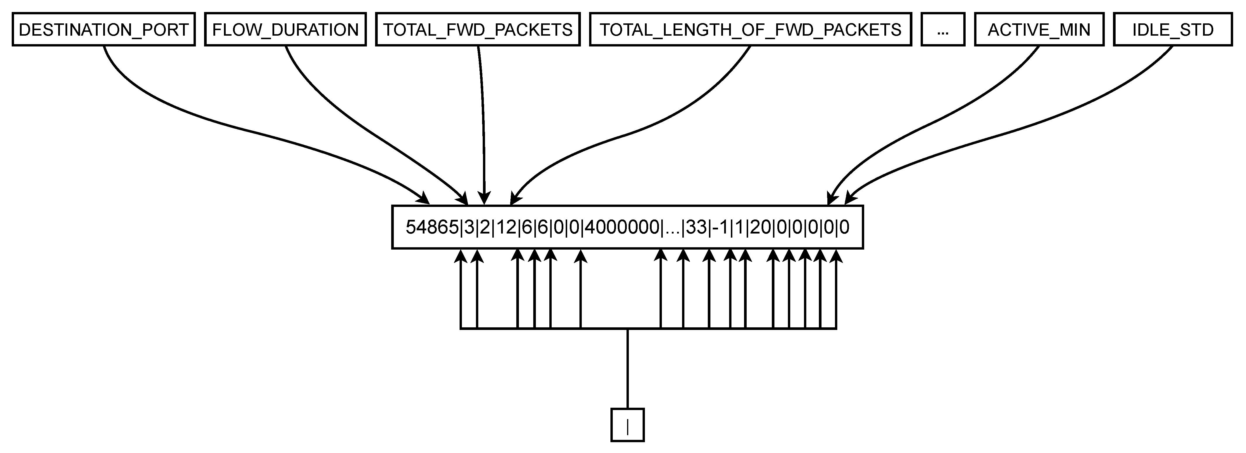
• Preparation of input strings: The T5 model, having been pre-trained on diverse NLP tasks, inherently requires string-based input for its “source_text” field. Our dataset, however, comprises 44 numerical features representing network flow statistics. To bridge this modality gap and enable the T5 model to process network flow data, we developed an abstract artificial language.
  This innovative design involves a two-step transformation process for each row of numerical data:

  -

  Feature-to-text conversion: Each numerical feature is individually converted into its string representation.

  -

  Sequential concatenation: These string representations of the features are then sequentially concatenated to form a single continuous input string. Inspired by the data representation strategy that we designed in a previous work [49], where adapted T5 for translation tasks involving multiple input features (such as jokes and puns) against a single model input, we used the vertical bar character (|) as a separator between each feature’s string value, following a predefined, consistent order.

  This process results in a unique character string for each network flow, effectively translating the numerical statistics of a network flow into a structured textual sequence. This abstract language allows the T5 model to process network flow data as if it were a specialized form of text, enabling the fine-tuning process to adapt the model’s powerful pattern recognition capabilities from linguistic structures to the complex patterns present in network flow statistics for cyberattack detection. Figure 3 shows an example of the construction of these input strings, given statistics of network flows. The top section displays the characteristics, while the bottom section shows the separator character. The central box presents a preprocessed input entry. Arrows indicate where each feature value is placed, alongside the vertical bar separating them.

  -

  Labeling: The labels with the types of attacks contained in the dataset are strings with alphanumeric characters, and, in this way, they are useful if the intention is to identify the type of attack at first sight. However, labels must be encoded to avoid issues in classification. We decided to encode the labels using sequential numbers, starting from 0.

2.3.2. Data Cleaning Results for CSE-CIC-IDS2018

The initial dataset consisted of 16,232,943 rows and 84 features. After cleaning, we had 15,705,343 rows and 45 columns, which were used to build our system.

Table 2. Summary of data cleaning results.

Step	Rows	Removed Rows	Columns	Removed Columns
Initial status	16,232,943		84
Removal of useless columns	16,232,943		80	4
Removal of columns with unique values	16,232,943		72	8
Removal of columns with high correlation	16,232,943		45	27
Removal of infinite, empty and null values	16,137,183	95,760	45
Removal of duplicate rows	15,705,343	431,840	45

shows a brief summary of the data cleaning results.

Table 3. Statistics of the data cleaning process by type of attack.

Types of Attacks	Initial Rows	After Cleaning	Removed Rows	Removed Proportion
Benign	13,484,708	13,352,392	132,316	0.98%
DDoS attacks-LOIC-HTTP	576,191	576,175	16	0.00%
DDOS attack-HOIC	686,012	668,461	17,551	2.56%
DoS attacks-Hulk	461,912	434,873	27,039	5.85%
Bot	286,191	282,310	3881	1.36%
Infiltration	161,934	160,604	1330	0.82%
SSH-Bruteforce	187,589	117,322	70,267	37.46%
DoS attacks-GoldenEye	41,508	41,455	53	0.13%
DoS attacks-Slowloris	10,990	10,285	705	6.41%
DDOS attack-LOIC-UDP	1730	1730	0	0%
Brute Force -Web	611	611	0	0%
Brute Force -XSS	230	230	0	0%
SQL Injection	87	87	0	0%
DoS attacks-SlowHTTPTest	139,890	19,462	120,428	86.09%
FTP-BruteForce	193,360	39,346	154,014	79.65%
	16,232,943	15,705,343	527,600	3.25%

shows a complete analysis after applying the entire data cleaning process to the selected dataset. The most interesting values are in bold. It is worth highlighting some aspects of interest. The labels SQL Injection, Brute Force-XSS, Brute Force-Web, and DDOS attack-LOIC-UDP lost no data rows. In addition, the most affected types were DoS attacks-SlowHTTPTest and FTP-BruteForce, since we removed 86.09% and 79.65% of the rows, respectively. Furthermore, the proportions across the attack types differ greatly.

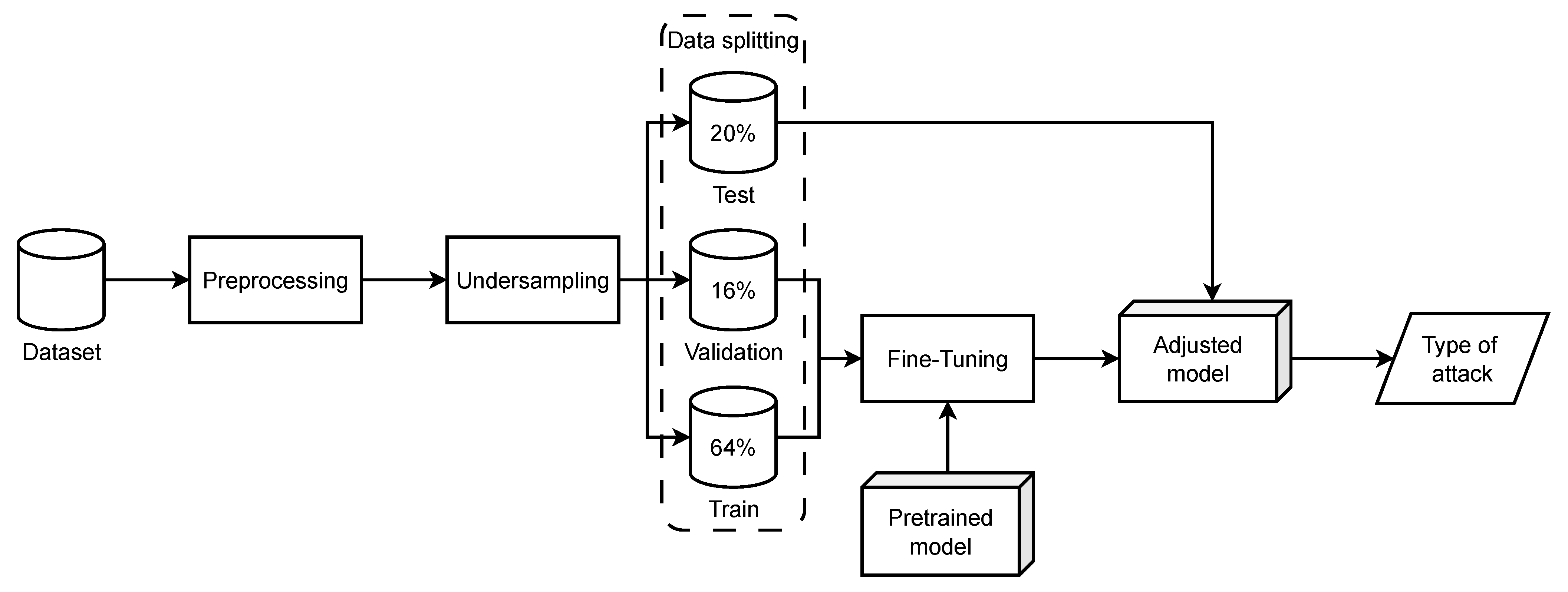
2.3.3. Undersampling

Table 4. Statistics of the data cleaning process grouped by benign/malignant.

Types of Attacks	Initial Rows	After Cleaning	Removed Rows	Removed Proportion
Benign	13,484,708	13,352,392	132,316	0.98%
Malignant	2,748,235	2,352,951	395,284	14.38%
	16,232,943	15,705,343	527,600	3.25%

contains an analysis similar to that performed for Table 3 but classifies the dataset into two types of network flows, that is, benign and malignant. The original dataset exhibited a significant class imbalance because the number of benign instances far exceeded the number of malignant ones. Originally, the dataset contained 13,484,708 benign rows and 2,748,235 malignant rows, accounting for 83.07% and 16.93%, respectively. The data cleaning process removed a substantial number of rows, but disproportionately affected the benign class. This further exacerbated the existing class imbalance. Even after cleaning, the dataset remained highly imbalanced, with 13,352,392 benign rows and 2,352,951 malignant rows. It is worth noting the proportion of data removed for both benign and malignant types of attacks, being 0.98% benign and 14.38% malignant, which corresponds to 132,316 and 395,284 rows, respectively.

Class imbalance can significantly impact the performance of machine learning models. Models trained on imbalanced datasets may become biased towards the majority class, leading to poor performance in the minority class. To address the severe class imbalance, the authors applied the undersampling technique, which is a widely used technique for addressing class imbalance. It involves reducing the number of instances in the majority class to match the number of instances in the minority class. Therefore, we agreed to balance the dataset with a proportion of approximately 50% benign data and 50% malignant data. We thus decided to randomly select 20% benign rows, resulting in a more balanced dataset, in terms of proportions between classes, and a balanced dataset in terms of proportions between benign and malignant data.

Table 5. Dataset statistics by type of attack after applying undersampling.

Types of Attacks	After Cleaning		Undersampling 20% Benign
	Rows	Prop.	Rows	Prop.
Benign	13,352,392	85.02%	2,670,478	53.16%
DDoS attacks-LOIC-HTTP	576,175	3.67%	576,175	11.47%
DDOS attack-HOIC	668,461	4.26%	668,461	13.31%
DoS attacks-Hulk	434,873	2.77%	434,873	8.66%
Bot	282,310	1.80%	282,310	5.62%
Infiltration	160,604	1.02%	160,604	3.20%
SSH-Bruteforce	117,322	0.75%	117,322	2.34%
DoS attacks-GoldenEye	41,455	0.26%	41,455	0.83%
DoS attacks-Slowloris	10,285	0.07%	10,285	0.20%
DDOS attack-LOIC-UDP	1730	0.01%	1730	0.03%
Brute Force -Web	611	0.004%	611	0.01%
Brute Force -XSS	230	0.001%	230	0.005%
SQL Injection	87	0.001%	87	0.002%
DoS attacks-SlowHTTPTest	19,462	0.12%	19,462	0.39%
FTP-BruteForce	39,346	0.25%	39,346	0.78%
	15,705,343		5,023,429

shows the final number of rows and their proportion for each class, after cleaning and after performing an undersampling of 20% benign network flows. The final proportions were slightly more balanced, since there are 53.16% benign rows, and the proportions of malignant labels increased by 313%. Therefore, after undersampling, the malignant types with the most rows had 13.31%, 11.47%, and 8.66%, for the classes DDOS attack-HOIC, DDoS attacks-LOIC-HTTP, and DoS attacks-Hulk, respectively.

Table 6. Dataset statistics grouped by benign/malignant after applying undersampling.

Types of Attacks	After Cleaning		Undersampling 20% Benign
	Rows	Prop.	Rows	Prop.
Benign	13,352,392	85.02%	2,670,478	53.16%
Malignant	2,352,951	14.98%	2,352,951	46.84%
	15,705,343		5,023,429

contains a similar analysis but classifies the rows as benign and malignant. After cleaning, the dataset had 13,352,392 benign rows and 2,352,951 malignant rows, which corresponds to 85.02% and 14.98%, respectively. At this point, the dataset had a pronounced imbalance. Hence, after applying the aforementioned undersampling of 20% benign rows of data, the proportions approached 53.16% benign network flows, with 46.84% being malignant.

The proportions resulting from the imbalance of the selected dataset are specified in Table 5 and Table 6. In addition to being useful for analyzing the distribution of data for each type of attack, these values are also useful to study the results, as well as to calculate the weighted metrics. It is worth highlighting that, in terms of rows per label, the dataset was still imbalanced, but slightly less than before, while in terms of proportions between benign and malignant network flows, the dataset was now balanced.

2.3.4. Data Splitting

At this point, we had a preprocessed dataset with two columns: source_text with the prepared input features, as explained in Section 2.3.1; and target_text with their labels. The only remaining step left was to separate the dataset into different subsets to correctly fine-tune each model. This means we needed training and validation subsets together to train each model and, finally, we needed the test subset, with data which each model had never seen, to subsequently obtain all the values for each metric. To achieve this, we split the preprocessed dataset using Cross-Validation (CV).

The agreed proportions were as follows. After performing a data shuffle, we fixed the first 80% to apply stratified fivefold CV, and the remaining 20% was fixed as the test subset. This means that for all folds in the CV, the test subset always contained the same collection of data rows.

Stratified fivefold CV [50] was applied as follows. In the first fixed 80% of the data, we divided it into 5 parts, and for each fold, the k-th part was selected as the validation subset, and the remaining 4 parts were selected as the training subset. That is, for the first fold, the first part, which contained 16% of the data, was selected as the validation subset, and the other 4 parts, which contained 64% of the data, were selected as the training subset. The remaining fixed 20% was considered as the test subset for all the folds.

In the case of the selected strategy, stratified means that each subset contained the same proportion of data rows for each label. The selected dataset contained a considerable amount of information. Therefore, in advance, applying this strategy might not have been necessary. Nevertheless, considering the presence of labels with very few rows of data, we decided to apply the strategy in order to obtain models that could classify these labels as accurately as possible.

2.3.5. Fine-Tuning Process

Training consists of adjusting the weights of each neuron of an ANN, such that predictions can be adjusted as closely as possible to the expected outputs. Fine-tuning involves using a pre-trained model as a starting point to solve a different problem. In essence, we load a pre-trained model and train it with our dataset, to adjust its weights to solve a new type of problem. Thus, instead of starting with a random weight configuration, we start with a weight configuration focused on solving a certain type of problem. In our case, the T5 model was pre-trained with the C4 [26] dataset, Colossal Clean Crawled Corpus, which was composed of hundreds of gigabytes of English text obtained from the Internet. Subsequently we applied fine-tuning with another dataset, focused on an entirely different scope, like that selected for our experiments.

Transfer Learning could be another option. This technique is similar to fine-tuning but with a particular difference. Fine-tuning updates all the weights of an ANN, unlike Transfer Learning, in which several layers are locked, such that they retain their weights, and only the weights of the unlocked layers are adjusted. Therefore, we decided to fine-tune all the weights, as the purpose of the model is being radically altered.

Once we had decided to fine-tune an existing snapshot of the T5 model, using the SimpleT5 [51] wrapper, the next step was to optimize the hyperparameters. SimpleT5 is a wrapper built over PyTorch 2.0.1, to perform fine-tuning of T5 without modifying its architecture. This package provides users with different functions to use different sizes of the T5 model by only developing a few lines of code. It contains functions for downloading pre-trained snapshots and assigning them to a new instance, training models, and predicting values or loading models previously trained with this package. SimpleT5 has several hyperparameters available for use, which we carefully analyzed to select the most appropriate values for some and identify others to be optimized. Once this task is completed, the fine-tuning of the model can be successfully executed. Therefore, SimpleT5, provides users with the following hyperparameters:

• max_epochs is the maximum number of epochs for the training step. It is set to 10, since LLMs have a high level of maturity and require relatively few epochs to achieve a good model. Therefore, after performing the preliminary experiments, we observed that the best-performing model of an experiment was never selected beyond the tenth epoch. Depending on the experiment, an overfitting could appear in one of the first epochs, even in the second one. Hence, 10 is a sufficiently large value.
• target_max_token_len contains the maximum number of output tokens. Since the selected model performs a classification task, it is unnecessary to set an excessively large value. It should be pointed out that the output of the model is a numerical value between 0 and 14. The maximum number of tokens is 512, which substantially exceeds the number typically required. Preliminary experiments concluded that the minimum number of tokens was 3 and we observed that the values for the selected metrics maintained the same trend for any value between 3 and 512. In addition, this parameter has the same behavior as the variable source_max_token_len parameter in terms of the relationship between the number of tokens and training time. Therefore, setting 3 as its value significantly reduces training times.
• batch_size is the parameter that contains the batch size to be used to train this model. The default value is 8 and values that are a power of 2 are typically used, such that values like 8, 16, or 32 are commonly used. The value 16 is set, which is a medium value, since it is neither the minimum nor is it too large.
• precision is the parameter that contains the training precision. The available values are double precision (64), full precision (32), or half precision (16). By default, this wrapper uses the value 32, which is the value used for the experiments. Here, 32 was selected because it is the central value, for instance, being neither the smallest nor the largest value.
• source_max_token_len contains the maximum number of input tokens, which, in this case, is 512 tokens. The larger the number of input tokens, the longer the training time, while the lower the value, the shorter the training time. Logically, a shorter training time is desired, so it is of interest to set this variable to the lowest possible value. However, given that the character strings used as input have an average of 189 characters, a minimum of 109, and a maximum of 345, it is important to consider that if too few tokens are selected, then the model will not take into account much of the input information needed for satisfactory task performance. Therefore, we must seek a balance, taking this parameter into account in the search for an optimal value that allows the model to be trained in the shortest possible time while keeping the selected metrics as high as possible. We planned to perform the optimization with 50, 100, 150, 200, 250, 350, and 500 tokens. The evaluation of the hyperparameter optimization process was carried out using the following evaluation metrics: accuracy, precision, recall, and F-score.

Table 7. Metrics for the hyperparameter optimization step.

Max. Input Tokens	Accuracy	Precision	Recall	F-score	Training Time
50	99.75%	99.75%	99.75%	99.75%	2:22:33
100	99.84%	99.84%	99.84%	99.84%	2:45:20
150	99.84%	99.85%	99.84%	99.84%	3:15:47
200	99.84%	99.85%	99.84%	99.84%	3:43:27
250	99.84%	99.85%	99.84%	99.84%	4:20:27
350	99.84%	99.85%	99.84%	99.84%	5:28:13
500	99.84%	99.85%	99.84%	99.84%	7:42:27

shows all the results in depth. It is worth highlighting the whole row for the value 150 of the maximum number of input tokens, since all values for all metrics for 150 are the best ones. The entire row is formatted in bold. This does not mean, however, that it is the best value, since all values for a greater maximum number of input tokens follow the same trend and differ slightly. Therefore, we added a new variable, which is the training time. It is important to note the increasing trend of this index, because the higher the number of input tokens, the longer the training time. Therefore, on the one hand, all values for all metrics for the value 150 are sufficiently stable to justify selecting it as the optimal value for the aforementioned hyperparameter, as it yields the best results for the selected metrics. On the other hand, it is also desirable to select a model that requires less training time. Hence, we chose the minimum value among the aforementioned candidates, which is 150.

3. Experimental Results

The experiments were performed in an environment with software that is commonly used for data science. We selected Python 3.8.17 to develop the experiments. All experiments were performed on the supercomputer of the University of Cádiz. It contains several NVIDIA A100 GPUs with 40GB of GPU memory and 256GB of RAM, each node with 2 CPUs and each with 64 cores. Moreover, it contains a number of nodes with more memory, more concretely with 1TB each node.

The hyperparameter optimization process led us to select the best value for the hyperparameter of the maximum number of input tokens. Using the best configuration for the training step, we performed a fine-tuning task using the stratified fivefold CV approach, which executes five different fine-tuning processes, each with its related pair of training and validation subsets. Each execution generates a snapshot that performs the classification between benign and malignant data and, in the second case, directly obtains the type of attack between the 14 types contained in the CSE-CIC-IDS2018 dataset. Since we configured the execution of 10 epochs, we obtained 10 model snapshots for each fold. Therefore, for each fold, we obtained the predictions using the validation subsets in order to select the best epoch, and finally, for the best one, we obtained the predictions using the test subset, which the model had never seen. We used these test predictions to calculate the values for each one of the selected metrics, for each fold. Finally, to complete the whole process, we calculated the mean and the standard deviation, for each metric.

The evaluation of the experiments published in this paper, as well as the hyperparameter optimization process, was carried out using the following evaluation metrics: accuracy, precision, recall and F-score. It is worth noting that we calculated the weighted metrics since the dataset is imbalanced, in terms of rows of data for each type of attack. In addition, these values allow us to compare our results with those reported in other publications. Considering the aforementioned information, we obtained 99.84%, for all the selected metrics.

The calculated metrics may not provide conclusive information under certain conditions. However, these metrics may conceal some information that could be interpreted in a confusion matrix.

Table 8. Confusion matrix, with y as rows and $\widehat{y}$ as columns, for CSE-CIC-IDS2018.

Label	Benign	DDoS Attacks-LOIC-HTTP	DDOS Attack-HOIC	DoS Attacks-Hulk	Bot	Infiltration	SSH-Bruteforce	DoS Attacks-GoldenEye	DoS Attacks-Slowloris	DDOS Attack-LOIC-UDP	Brute Force -Web	Brute Force -XSS	SQL Injection	DoS Attacks-SlowHTTPTest	FTP-BruteForce
Class	0	1	2	3	4	5	6	7	8	9	10	11	12	13	14	Misclassified
0	532,635	19	0	0	14	1,420	5	0	0	0	3	0	0	0	0	0.27%
1	4	115,231	0	0	0	0	0	0	0	0	0	0	0	0	0	0%
2	0	0	133,692	0	0	0	0	0	0	0	0	0	0	0	0	0%
3	0	0	0	86,975	0	0	0	0	0	0	0	0	0	0	0	0%
4	5	0	0	0	56,457	0	0	0	0	0	0	0	0	0	0	0.01%
5	72	0	0	0	0	32,049	0	0	0	0	0	0	0	0	0	0.22%
6	0	0	0	0	0	0	23,464	0	0	0	0	0	0	0	0	0%
7	1	0	0	0	0	0	0	8290	0	0	0	0	0	0	0	0.01%
8	0	0	0	0	0	0	0	0	2057	0	0	0	0	0	0	0%
9	0	0	0	0	0	0	0	0	0	346	0	0	0	0	0	0%
10	7	0	0	0	0	0	0	0	0	0	106	7	2	0	0	13.11%
11	3	0	0	0	0	0	0	0	0	0	0	42	1	0	0	8.7%
12	5	0	0	0	0	0	0	0	0	0	1	7	4	0	0	76.47%
13	0	0	0	0	0	0	0	0	0	0	0	0	0	3892	0	0%
14	0	0	0	0	0	0	0	0	0	0	0	0	0	0	7869	0%

shows the confusion matrix for the first fold. The results are highly optimistic since the higher values are in the main diagonal and the remaining values are 0 or close to 0. In addition, two interesting conclusions were extracted from this matrix. The first is the number of false negatives that appear when the model predicted Infiltration, label number 5, where the right answer is Benign, label number 0. This means that, for the model, both classes are confusing for a minimum proportion of data.

The other interesting finding is that the model exhibited lower recall and precision for certain minority classes within the datasets. For instance, SQL Injection attacks, representing an extremely low proportion of the total instances (only 17 samples), achieved a detection accuracy of merely 23.53%. Similarly, Brute-Force-Web attacks, with 122 samples, showed an accuracy of 86.89%, and Brute-Force-XSS attacks, with 46 samples, reached 91.3%. While the latter two showed reasonable accuracy given their sample sizes, their performance was still impacted by their minority status compared to the overall dataset. This indicates that the primary challenge for these specific attack types lies in the severe data imbalance at the sub-category level. The limited availability of training data for some types of attacks hinders the capacity of LLMs to classify them accurately, leading to an increased number of false negatives or misclassifications, particularly for SQL Injection, Brute Force-Web and Brute Force-XSS.

Appendix A contains and describes the confusion matrices for the CIC-IDS-2017 and BCCC-CIC-IDS-2017 datasets.

An initial analysis of the confusion matrix for the CSE-CIC-IDS2018 dataset was conducted, from which we extracted interesting information. The next step of our analysis was to study the effectiveness of our system using the aforementioned metrics, namely, accuracy, precision, recall, F-score, and some critical cybersecurity-specific metrics such as False-Positive Rate (FPR), False-Negative Rate (FNR), and Detection Latency. Without these metrics, we cannot verify whether our methodology is valid regardless of the dataset used.

Table 9. Results of our approach for different datasets.

Dataset	Accuracy	Precision	Recall	F-score	FPR	FNR	Detection Latency
CIC-IDS-2017	99.94%	99.94%	99.94%	99.94%	0.01%	0.05%	0.035 s
CSE-CIC-IDS2018	99.84%	99.84%	99.84%	99.84%	0.27%	0.02%	0.032 s
BCCC-CIC-IDS-2017	99.90%	99.90%	99.90%	99.90%	0.11%	0.04%	0.037 s

displays all the results for all the selected metrics, using the previously studied CSE-CIC-IDS2018, as well as CIC-IDS-2017 and BCCC-CIC-IDS-2017.

We obtained the best results when applying our methodology to the CIC-IDS-2017 dataset. We obtained 99.94% for all the metrics, which is 0.1% better than applying it to CSE-CIC-IDS2018. Regarding the augmented dataset, we obtained 99.9% for all the metrics applying our approach to BCCC-CIC-IDS-2017. Considering that this dataset contains a larger set of features, we obtained results that were 0.04% worse than those achieved with the original dataset, CIC-IDS-2017. Nonetheless, we can see that all the results are relatively consistent and present promising values according to the metrics selected for this study.

On the other hand, the CIC-IDS-2017 also demonstrated an exceptionally low FPR of only 0.01%, indicating a minimal rate of false alarms, which is crucial for reducing alert fatigue in operational security centers. Furthermore, its FNR of 0.05% underscores the model’s high effectiveness in detecting actual attacks, significantly reducing the risk of missed threats. For CSE-CIC-IDS2018, it recorded an FPR of 0.27% and an FNR of 0.02%. Although its FPR is higher than for CIC-IDS-2017, it remains within an acceptable range for many security operations. Its FNR is particularly low, indicating robust detection of true positives. The BCCC-CIC-IDS-2017 also maintained a highly respectable FPR of 0.11% and an FNR of 0.04%.

Figure 4 displays the progression of the training loss, validation loss, and validation accuracy over ten epochs for our models trained on the CSE-CIC-IDS2018, CIC-IDS-2017, and BCCC-CIC-IDS-2017 datasets. A clear decrease in both loss values is observed within the first two epochs, indicating that the model rapidly learns the fundamental patterns from the data. Following this initial phase, both the training loss and validation loss curves converge and stabilize at very low values. Notably, the validation loss remains consistently low and does not exhibit an upward trend as training progresses, which would be a clear indicator of overfitting. This behavior provides strong evidence that the three models generalize effectively to unseen data and do not present overfitting.

Simultaneously, the validation accuracy curve shows a rapid initial increase, stabilizing at very high values, which complements the information provided by the loss curves. This consistent behavior across all three datasets provides strong evidence that our models not only learn effectively from the training data but also generalize robustly to unseen data and do not suffer from overfitting.

Concerning detection latency, our system consistently demonstrated efficient processing times across all datasets. The CIC-IDS-2017 showed an average latency of 0.035 s, compared to 0.032 s for CSE-CIC-IDS2018, and 0.037 s for BCCC-CIC-IDS-2017. These low latency values highlight the potential for integrating our LLM-based solution into systems requiring timely threat analysis.

Overall, despite minor variations, the results across all datasets are remarkably consistent and demonstrate highly promising values for all selected metrics, underscoring the robustness and reliability of our proposed LLM-based cyberattack detection approach.

At this stage, we can thus compare our results with the aforementioned research papers. This comparison focuses on widely accepted performance metrics, including accuracy, precision, recall, F1-score, FPR, and FNR. It is important to note that direct comparisons of detection latency were not feasible due to variations in the hardware environments used for model training and inference reported in the respective literature, which could significantly skew such comparisons. Therefore, our focus remains on the efficacy of detection.

We already demonstrated the validity of our methodology across different datasets. Section 4 compares our approach with different strategies published in other research papers.

4. Related Work

To provide an overview of the published papers on cyberattack detection models, Section 4.1 describes the strategies based on LLM, while Section 4.2 details the ML (non-LLM) techniques [52]. In Section 4.3, we compare our approach with others already published by other authors using the selected metrics.

4.1. Strategies Based on LLM

In this paper, we present a new approach, namely, the detection of cyberattacks based on the fine-tuning of an encoder–decoder model pre-trained for NLP tasks. Regarding our approach, we found a limited number of papers related to NIDS based on an LLM, using the CSE-CIC-IDS2018 dataset, presented in this section. Two papers are based on an encoder-only model and the other on encoder-only and decoder-only models. Moreover, we include two papers based on the same line of research, but using a different dataset.

Manocchio et al. [28] introduced FlowTransformer, which is a transformer framework for flow-based NIDS. They used three datasets for the study of results: CSE-CIC-IDS2018, NSL-KDD and UNSW_NB15. They used different approaches and two well-known transformer architectures, GPT 2.0 and BERT. These are decoder-only and encoder-only LLMs, respectively. In contrast, our proposed approach uses the T5 model, which is based on an encoder–decoder architecture. For the CSE-CIC-IDS2018 dataset, using the GPT-based model, they obtained an accuracy of 95.86% and an F-score of 96.93%, and for the BERT-based model, they obtained an accuracy of 95.48% and an F-score of 95.80%.

Li et al. [27] presented the Conditional Generative Adversarial Network (CGAN), used together with BERT, for intrusion detection. Beyond the architectural differences previously discussed, another significant distinction between our approach and other LLM-based methodologies lies in the handling of data imbalance and the nature of the data used for training. The CGAN was used to balance the dataset with data augmentation. We used original data, since we performed an undersampling of the majority class, while they used synthetic data. They presented results after testing their approach with the datasets NF-ToN-IoT-V2, NF-UNSW-NB15, and CSE-CIC-IDS2018. However, in their study, we did not find all the original types of attacks for the latter dataset, which is that used for our research. Finally, they prepared a comparison between the three aforementioned datasets using different methods. For the CSE-CIC-IDS2018 dataset, using their proposed approach, they obtained 98.22% accuracy, 98.25% precision, 98.22% recall, and 98.23% F-score. For the other methods, their accuracies are between 86.07% and 96.83%, precision rates between 85.91% and 97.46%, recall rates between 86.07% and 96.83%, and an F-score between 84.39% and 97.01%.

The references mentioned in the previous two paragraphs are the only ones working on an LLM-based approach, for the detection of cyberattacks, using the same dataset as in the present study. After comparing both studies and our proposed approach, we can assert that our results are superior, as we explain in Section 4.

Ferrag et al. [29] presented an architecture based on BERT, called SecurityBERT, obtaining 98.2% accuracy and 98% precision, recall, and F-score. They reported an inference time of 0.15 s on an average CPU and a compact model size of 16.7MB. They introduced a privacy-preserving BERT-based lightweight model designed specifically for cyber threat detection in IoT/IIoT devices. Their approach, while also leveraging a transformer architecture (BERT, an encoder-only model), includes a unique information encoding layer aimed at preserving data privacy, which is a critical concern in resource-constrained and sensitive IoT environments. This specialization for IoT/IIoT networks, driven by specific privacy requirements, distinguishes their work. In contrast, our study focuses on a more general NIDS, using an encoder–decoder model, T5, for broad cyberattack detection on standard network flow statistics, without the specific privacy-preserving layers tailored for IoT constraints. They only used the Edge-IIoTset dataset, which contains network traffic, but is focused on IoT.

Lira et al. [53] presented a model called BERTIDS, based on BERT. This paper was published in 2024 but only used the NSL-KDD dataset, published in 2009. The authors published a comparative table with other approaches, which obtained accuracies of no more than 90%. They obtained 98.01% accuracy, 98.31% precision, 98.01% recall and 98.09% F-score. In this sense, it is not comparable to our results as they are different datasets and different models, but the following can be highlighted: we used a more modern dataset (with the most up-to-date and popular types of attacks); our model is based on a more modern model (both are LLM, both created by Google, but BERT was published in 2018 and T5 in 2019), BERT is an encoder-only model and T5 is an encoder–decoder model; and our accuracy is higher than 98.01%.

The results of the latter two papers are not directly comparable with our research, since they used different datasets.

4.2. Other Strategies Non-LLM Based on ML

Given there are few research papers related to our approach, we present some of the latest research results related to NIDS, which use different AI techniques. In order to analyse related works, we focus on strategies that make use of the selected dataset, so as to be able to compare the effectiveness of our proposal.

Macas et al. [5] published an interesting survey, which lists the most widely used techniques for each cybersecurity field. One of these is related to NIDS; they also introduced different AI techniques, none of which used, however, models based on NLP. Nonetheless, they mentioned BERT, in addition to GPT-3, but for SPAM detection. This survey references two interesting papers: Abdel-Basset et al. [12] proposed a Semi-Supervised DL approach for Intrusion Detection (SS-Deep-ID) with the following results for CSE-CIC-IDS2018: 98.71% accuracy, 94.91% precision, 94.30% recall, and 94.92% F-score. Their results were the following using the CIC-IDS-2017 dataset: 99.69% accuracy, 92.31% precision, 96.29% recall, and 94.18% F-score. They compared their results with other papers. With their proposal obtaining the best results for the metrics they selected. In the other cited paper, Nie et al. [13] proposed a Generative Adversarial Network (GAN)-based approach, using the CSE-CIC-IDS2018 dataset. They reported a 95.32% accuracy, 99.88% precision, 95.85% recall, and 97.30% F-score. They also compared their results with different approaches found in other publications.

Wang et al. [22] proposed a Genetic Algorithm with a Back Propagation Neural Network (GA-BPNN) model for computer network safety. They applied their approach to the CIC-IDS-2017 datasets. Their results were 98% accuracy, 98.5% precision, 95% recall and 96.5% F-score.

Maruthupandi et al. [11] introduced an Intelligent Attention-Based Deep Convoluted Learning (IADCL) model. They applied their approach to different datasets, such as, NSL-KDD, CIC-IDS-2017, and CSE-CIC-IDS2018. They compared their results with other approaches they applied, including Immune Net, eXtreme Gradient Boosting (XGBoost), Random Forest (RF), Decision Tree (DT), and Logistic Regression (LR). Considering the aforementioned techniques, that is, first their proposed approach and then the other approaches, their results when applying CSE-CIC-IDS2018 in terms of accuracy were 98.70%, 99.63%, 99.09%, 98.81%, 98.54%, and 92.96%; 99.72%, 99.64%, 99.03%, 98.82%, 93.41%, and 98.80% precision; 99.70%, 99.63%, 99.07%, 98.81%, 96.76%, and 90.96% recall; and an F-score of 99.71%, 99.63%, 99.07%, 98.81%, 95.06%, and 90.87%, respectively. Meanwhile, for CIC-IDS-2017, they reported 99.70%, 99.63%, 99.09%, 98.81%, 98.54%, and 92.96% accuracy; 99.72%, 99.64%, 99.03%, 98.82%, 93.41%, and 90.80% precision; 99.70%, 99.63%, 99.07%, 98.81%, 96.76%, and 90.96% recall; and an F-score of 99.71%, 99.63%, 99.07%, 98.81%, 95.06%, and 90.87%, respectively.

Guo et al. [23] introduced a 1D-TCN-ResNet-BiGRU-Multi-Head Attention (TRBMA)-based model, more concretely TRBMA (BS-OSS), a variant of the TRBMA model that integrates borderline SMOTE-OSS hybrid sampling, applying their approach to the CIC-IDS-2017 dataset. Their results were 99.88% accuracy, 99.86% precision, 99.88% recall, and 99.89% F-score.

Hariharan et al. [24] proposed a hybrid DL model for NIDS using Seq2Seq and ConvLSTM-Subnets, applied to the CIC-IDS-2017 dataset. Their results were 99% accuracy, 97% precision, 96% recall, and 97% F-score.

Vo et al. [54] introduced an approach based on Augmented Wasserstein GAN (AWGAN) and Parallel Ensemble Learning-based Intrusion Detection (PELID) algorithms, known as APELID. They used the CSE-CIC-IDS2018 and NSL-KDD datasets for their study. Their results, after applying their approach with the first dataset, were 99.99% for all the metrics: accuracy, precision, recall, and F-score. This strategy is characterized by balancing the dataset using a GAN, generating synthetic data to improve training. This means that we cannot compare our results with those published in this paper since we do not use the same data to train our model.

Amin et al. [55] proposed Chaotic Zebra Optimization Algorithm and Long Short-Term Memory (CZOLSTM) for the detection of cyberthreats. They used the CSE-CIC-IDS2018 dataset and their results were 99.92% accuracy and 99.94% precision, recall and F-score. They made a binary classification between benign and malignant data, and, in addition to taking just malignant data, developed a classification from a subset of types of attacks contained in the original dataset. Therefore, our results cannot be compared with theirs.

Kunang et al. [14] proposed a hybrid DL model for an IDS on the IoT platform. For this study, they used the Bot-IoT and CSE-CIC-IDS2018 datasets. For their proposal, and using the latter dataset, their results were 99.17% accuracy, 99.26% precision, 99.17% recall, and 99.2% F-score.

Bhardwaj et al. [15] proposed a framework based on a Convolutional Neural Network (CNN). They used different datasets, such as CSE-CIC-IDS2018, UNSW-NB15, and CIC-Darknet2020. For the first dataset, they obtained a 99.4% of accuracy, using their proposed framework.

Wang et al. [16] presented an Attention-based CNN for IDS. They carried out their research using CSE-CIC-IDS2018. For their proposed model, they obtained 99.36% accuracy. They reported no results on other metrics.

Tapu et al. [17] proposed a novel idea of hybrid meta-DL to detect malicious packet data. They used a combination of Siamese and Prototypical networks, where the first was used for binary classification and the latter for multiclass classification. For their hybrid meta-approach, using the CSE-CIC-IDS2018 dataset, their results were 90.64% accuracy, 91.66% precision, 90.64% recall and 91% F-score. Additionally, using CIC-IDS-2017, their results were 95.68% accuracy, 96.50% precision, 95.68% recall and 96.10% F-score.

Li et al. [18] proposed the Hierarchical and Dynamic Feature Extraction Framework (HDFEF) for IDS. They presented results for different datasets as CIC-IDS-2017, UNSW-NB15, and CSE-CIC-IDS2018. For the first dataset, they obtained 99.73% precision, 99.96% recall and 99.84% F-score. For the latter dataset, they obtained 98.22% precision, 99.77% recall and 98.49% F-score. They reported no results about accuracy.

Yilmaz et al. [19] used different approaches for NIDS, including RF, CatBoost, LightGBM and XGBoost, applied to different datasets, such as CIC-IDS-2017, CSE-CIC-IDS2018, and INSDN. Regarding their results with the CSE-CIC-IDS2018 dataset, using RF, they obtained 93% precision, 71% recall, and 74% F-score; using CatBoost, they obtained 89%, 83%, and 83%, respectively; and using LightGBM they obtained 87%, 84%, and 85%, respectively. Finally, with XGBoost, they obtained 89%, 85%, and 86% respectively. They presented no results related to accuracy. For CIC-IDS-2017, using RF, they obtained 93% precision, 71% recall, and 74% F-score; using CatBoost, they obtained 89%, 83%, and 83%; using LightGBM, they obtained 87%, 84%, and 85%; and using XGBoost, they obtained 89%, 85%, and 86%, all respectively. No results were reported for accuracy.

Hammad et al. [20] proposed a classifier using an approach called Multinomial Mixture Modeling with Median Absolute Deviation and RF (MMM-RF). They used the CSE-CIC-IDS2018 dataset and obtained 99.98% of accuracy with their approach. They presented no results for other metrics.

Yu et al. [21] presented a Packet Bytes-based CNN (PBCNN) for NIDS. They used CSE-CIC-IDS2018, with their results being 99.99% accuracy, 98.2% precision, and 98.3% recall and F-score.

4.3. Comparative Analysis

This section details the comparison between our approach and other strategies published by other authors. More concretely, in Section 4.3.1, we compare our results with other studies which used the CSE-CIC-IDS2018 dataset, while Section 4.3.2 compares with CIC-IDS-2017. Unfortunately, we cannot compare our results for BCCC-CIC-IDS-2017 with other approaches because we were unable to find any studies, since this latter dataset is new.

4.3.1. Using the CSE-CIC-IDS2018 Dataset

Section 4.1 and Section 4.2 contain details on the publications included in this comparative study.

Table 10. Results for the selected metrics using CSE-CIC-IDS2018.

Reference	Technique	Accuracy	Precision	Recall	F-score	FPR	FNR
Our approach	T5	99.84%	99.84%	99.84%	99.84%	0.27%	0.02%
Li et al. [27]	CGAN + BERT	98.22%	98.25%	98.22%	98.23%	–	–
Manocchio et al. [28]	GPT 2.0	95.86%	–	–	96.93%	0.11%	–
	BERT	95.48%	–	–	95.80%	0.47%	–
Maruthupandi et al. [11]	IADCL	99.82%	99.80%	99.81%	99.80%	–	–
	Immune Net	99.78%	99.77%	99.78%	99.70%	–	–
	XGBoost	99.00%	99.03%	99.00%	99.01%	–	–
	RF	98.81%	98.82%	98.81%	98.81%	–	–
	DT	98.69%	93.41%	98.79%	96.03%	–	–
	LR	87.96%	90.80%	87.96%	88.99%	–	–
Abdel-Basset et al. [12]	SS-Deep-ID	98.71%	94.91%	94.30%	94.92%	–	–
Nie et al. [13]	GAN	95.32%	99.88%	95.85%	97.30%	0.89%	–
Kunang et al. [14]	Hybrid DL Model	99.17%	99.26%	99.17%	99.20%	0.18%	–
Bhardwaj et al. [15]	CNN-1D	99.40%	–	–	–	–	–
Wang et al. [16]	CNN	99.36%	–	–	–	0.16%	0.79%
Tapu et al. [17]	Hybrid DL Model	90.64%	91.66%	90.64%	91.00%	–	–
Li et al. [18]	HDFEF	–	98.22%	99.77%	98.49%	–	–
Yilmaz et al. [19]	RF	–	94.00%	76.00%	79.00%	0.53%	–
	CatBoost	–	91.00%	80.00%	83.00%	0.43%	–
	LightGBM	–	91.00%	81.00%	83.00%	0.42%	–
	XGBoost	–	89.00%	83.00%	84.00%	0.42%	–
Hammad et al. [20]	MMM-RF	99.98%	–	–	–	0.02%	–
Yu et al. [21]	PBCNN	99.99%	98.20%	98.30%	98.30%	–	–

shows the results published in these papers and in ours, after applying our approach to the CSE-CIC-IDS2018 dataset. Beyond standard metrics such as accuracy, precision, recall, and F-score, this comparison critically includes the FPR and FNR, which are paramount for assessing the operational viability of an IDS. This table is divided into three parts by dark horizontal lines. The first part, with only one row, contains the results of our approach. Our approach, utilizing the T5 model, achieves a leading accuracy of 99.84%, demonstrating its strong overall performance. More importantly for real-world deployment, our model exhibits a highly competitive FPR of 0.27% and a remarkably low FNR of 0.02%.

The second part shows the results of two approaches based on LLM and the same dataset we used. Our results are at least one percentage unit better than the others, for the metrics of accuracy, precision, recall, and F-score. Therefore, our approach performs better than those in the aforementioned papers, and it is worth noting that we selected the smallest size of the available snapshots of the T5 model. Regarding FPR and FNR, our system demonstrates a robust balance. For instance, while Manocchio et al. [28], GPT 2.0 shows a lower FPR of 0.11%, and their overall accuracy (95.86%) is considerably lower, suggesting a trade-off in broader detection capability. Conversely, their BERT model yields a 0.47% higher FPR than ours.

Finally, in the last part of the table mentioned above, we can find several references regarding IDS-related models that used ML techniques, non-LLM, and the same dataset we used. Our results are again better. Considering that we selected the smallest available size of the T5 model, we can assert that our results for all metrics are better than most of the papers found. Only two approaches, that is [20,21], obtained superior accuracies, and only another, namely [13], obtained slightly better precision. In the case of Yu et al. [21], although accuracy is better, for the other metrics, their values are poorer than ours. In this sense, Harrell [56] affirms that accuracy can be a misleading metric for imbalanced datasets. Therefore, our system can be said to perform better. As for Hammad et al. [20], although their accuracy is higher, this alone is not informative without other metrics; hence we cannot conclude their approach is more effective than ours.

Regarding FPR and FNR, Nie et al. [13] reported an FPR of 0.89%, and Yilmaz et al. [19], with various ML models, reported higher FPR values, ranging from 0.42% to 0.53%. Our model also compares favorably with Wang et al. [16], where our FNR is significantly lower, indicating fewer missed attacks despite a slightly higher FPR. Notably, Hammad et al. [20] achieves a lower FPR, but full comparative metrics for a balanced assessment are not available.

Figure 5 provides a detailed visual analysis of the performance of our proposed approach and other comparative strategies, illustrating the difference of each metric relative to the absolute best value observed within each dataset CSE-CIC-IDS2018. For metrics not reported in the original comparative studies, a value of -1 is assigned for visualization purposes. This clearly distinguishes non-comparable data points, indicating that the original work did not provide these specific performance indicators, rather than implying a negative performance. A shorter bar or one closer to zero indicates that the proposal achieves the best performance or is very close to it for that specific metric. We can observe that for accuracy, precision, recall, and F-score metrics, our T5 approach consistently positions itself as one of the best or the outright best, exhibiting minimal (or zero, as for recall and F-score) differences compared to the maximum value achieved. This highlights our model’s high capability for general classification and effective attack identification.

The consistently low FNR of our T5 model, especially in conjunction with its high accuracy and competitive FPR, highlights its superior ability to minimize missed attacks while keeping false alarms at an acceptable level, thus offering a more balanced and practical solution for threat detection. Therefore, our approach performs the best among the LLM-based research papers, and our results compared to the other ML-based techniques, are better for all the metrics, with the exception of a pair of studies, over which we obtained better results for most of the selected metrics.

4.3.2. Using the CIC-IDS-2017 Dataset

Section 4.2 contains details on the publications included in this comparative analysis.

Table 11. Results for the selected metrics using CIC-IDS-2017.

Reference	Technique	Accuracy	Precision	Recall	F-Score	FPR	FNR
Our approach	T5	99.94%	99.94%	99.94%	99.94%	0.01%	0.05%
Maruthupandi et al. [11]	IADCL	99.70%	99.72%	99.70%	99.71%	–	–
	Immune Net	99.63%	99.64%	99.63%	99.63%	–	–
	XGBoost	99.09%	99.03%	99.07%	99.07%	–	–
	RF	98.81%	98.82%	98.81%	98.81%	–	–
	DT	98.54%	93.41%	96.76%	95.06%	–	–
	LR	92.96%	90.80%	90.96%	90.87%	–	–
Abdel-Basset et al. [12]	SS-Deep-ID	99.69%	92.31%	96.29%	94.18%	–	–
Tapu et al. [17]	Hybrid DL Model	95.68%	96.50%	95.68%	96.10%	–	–
Li et al. [18]	HDFEF	–	99.73%	99.96%	99.84%	–	–
Yilmaz et al. [19]	RF	–	93.00%	71.00%	74.00%	0.14%	–
	CatBoost	–	89.00%	83.00%	83.00%	0.02%	–
	LightGBM	–	87.00%	84.00%	85.00%	0.01%	–
	XGBoost	–	89.00%	85.00%	86.00%	0.02%	–
Wang et al. [22]	GA-BPNN	98.00%	98.50%	95.00%	96.50%	–	–
Guo et al. [23]	TRBMA (BS-OSS)	99.88%	99.86%	99.88%	99.89%	–	–
Hariharan et al. [24]	Hybrid DL Model	99.00%	97.00%	96.00%	97.00%	–	–

displays the results reported in these papers and ours, after applying our approach to the CIC-IDS-2017 dataset. This table is divided into two parts by dark horizontal lines. The first part, with only one row, contains the results of our approach. Our T5-based approach demonstrates exceptional performance on CIC-IDS-2017, achieving 99.94% across all core metrics. Crucially, it records an extremely low FPR of 0.01%, signifying an almost negligible rate of false alarms, which is a highly desirable characteristic for operational security. Concurrently, its FNR of 0.05% underscores its robust ability to identify actual threats, minimizing the risk of undetected attacks.

The second part shows several references for IDS-related models that used ML techniques, since we found no studies on LLM, using CIC-IDS-2017. Our results are again better. Considering we selected the smallest available size of the T5 model, we can state that our results for all metrics are better than almost all the papers found. Only one approach, that of Li et al. [18], obtained slightly better recall. When examining the error rates of other methods that report FPR, our model generally maintains a competitive or superior balance. For instance, while some traditional ML models from Yilmaz et al. [19] achieve very low FPRs, not better than ours, their corresponding recall values are significantly lower than those of our model, implying a higher risk of missed attacks, which suggests higher FNR, although this was not reported by the authors.

Figure 6 extends this comparative analysis to the CIC-IDS-2017 dataset, using the same perspective as Figure 5. Consistent with our findings on CSE-CIC-IDS2018, our approach continues to demonstrate its strength across accuracy, precision, recall, and F-score. The consistently minimal (or zero) differences from the best-observed values reaffirm the robustness and superior performance of our model for cyberattack detection across different benchmark datasets.

Our model’s capacity to achieve near-perfect core metrics alongside such a low FPR and FNR highlights its comprehensive and balanced detection capability. Therefore, our approach performs best among the ML-based techniques.

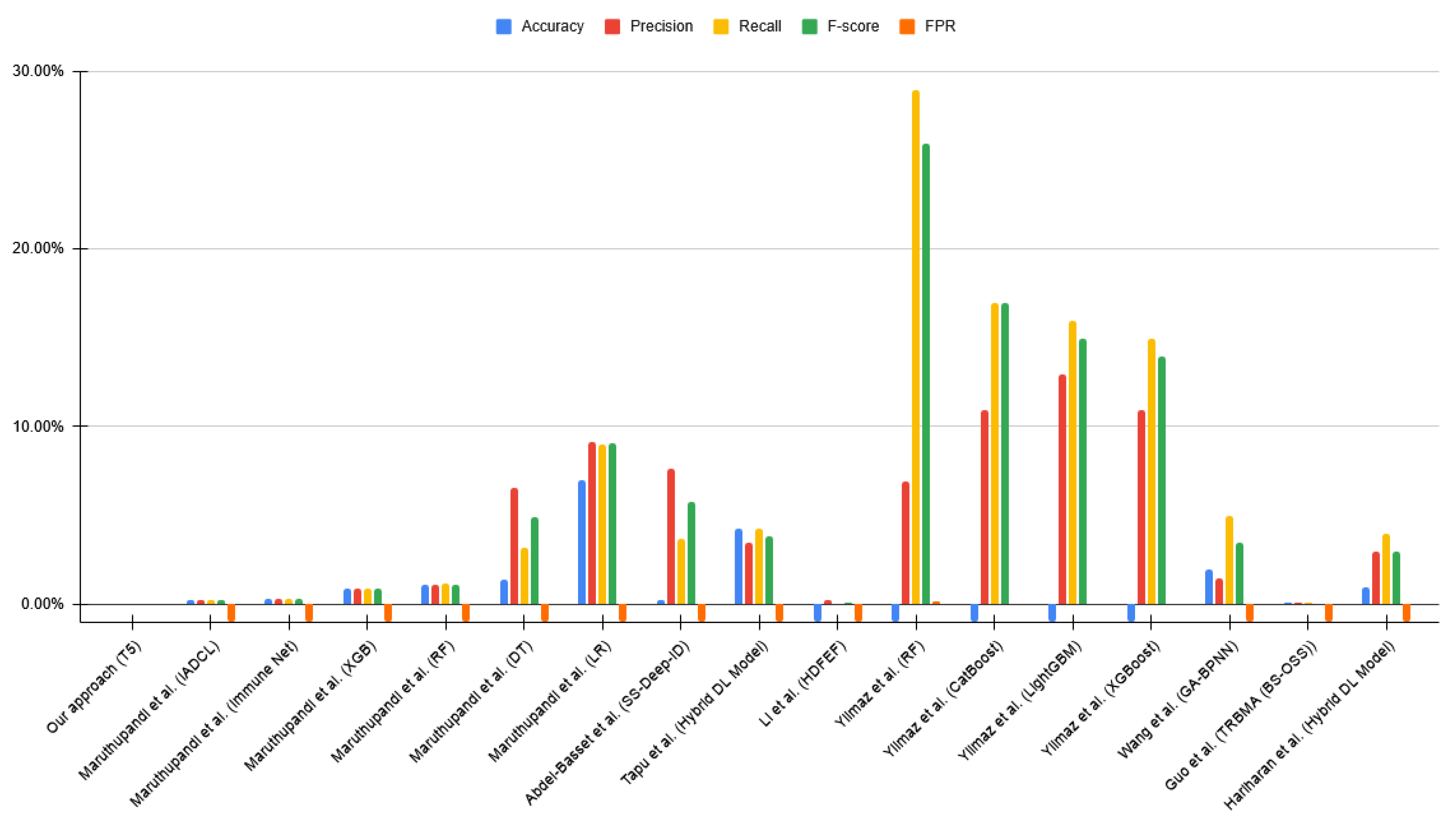
4.3.3. Using the BCCC-CIC-IDS-2017 Dataset

Finally, we unfortunately found no studies with results after applying the BCCC-CIC-IDS-2017 dataset, since it was launched while the present study was under development.

5. Conclusions and Future Work

The dynamic and increasing range of cyberattacks presents a significant challenge to current security systems, necessitating the development of new strategies for robust threat detection.

The current study presented a novel approach for cyberattack detection using an encoder–decoder pre-trained LLM, fine-tuned to adapt its classification scheme for the detection of cyberattacks. Given statistics of already finished network flows, we built an anomaly-based system for the detection of cyberattacks. We presented a novel methodology based on the adaptation of the original tasks of an LLM from NLP to detect cyberattacks. Our first contribution is to convert the numerical network flow statistics into a consistent abstract artificial language input string to be interpreted by the LLM.

We validate the robustness of our detection system across three diverse and widely recognized datasets, CSE-CIC-IDS2018, CIC-IDS-2017, and BCCC-CIC-IDS-2017. By using undersampling and a Stratified Fivefold Cross-Validation approach, our model achieved consistently high performance across all evaluated datasets. Specifically, for the CIC-IDS-2017 dataset, we obtained accuracy, precision, recall, and F-score of more than 99.94%. For CSE-CIC-IDS-2018, these metrics exceeded 99.84%, and for BCCC-CIC-IDS-2017, they were all above 99.90%. These results collectively demonstrate superior performance for cyberattack detection, while maintaining highly competitive FPR and FNR, ensuring both minimal false alarms and robust threat identification. Crucially, the consistent convergence of training and validation loss, alongside stable high validation accuracy across all datasets, provides strong empirical evidence that our model generalizes effectively to unseen data and does not suffer from overfitting. This efficacy is achieved by relying exclusively on real-world network flow statistics, without the need for synthetic data generation, differentiating our approach from those that may use synthetic data for training.

Future Work

Future work will focus on several key directions aimed at refining current capabilities and addressing identified limitations.

A primary focus will be the mitigation of the effectiveness limitations observed for attack types that are poorly represented in the dataset, which currently leads to a higher FNR (as detailed in our granular analysis of the confusion matrix in Section 3 with SQL Injection, Brute Force-Web and Brute Force-XSS). To address this issue, we plan to conduct a comprehensive study on the application of advanced data augmentation and oversampling techniques specifically tailored for highly imbalanced cybersecurity datasets. This will involve exploring methods such as Synthetic Minority Oversampling Technique (SMOTE) and Adaptive Synthetic Sampling (ADASYN). The objective is to enrich the dataset for these under-represented attack categories, providing the LLM with a more robust and diverse set of training examples.

While our current system effectively uses the T5 encoder–decoder architecture, future work will involve exploring and comparing various LLM architectures and model sizes. This includes investigating the performance trade-offs of smaller, more efficient T5 variants for potential edge deployments, as well as evaluating other encoder–decoder models or even novel hybrid architectures. The aim is to optimize the balance between detection performance and computational efficiency for diverse operational environments, particularly for low-resource settings.

We selected fine-tuning to perform our experiments. Our strategy achieved better results than other approaches mentioned in Section 4. However, it would be interesting to study the differences between the application of fine-tuning or Transfer Learning. Therefore, we propose to apply the latter approach in order to determine which is better in our case.

To enhance the scalability and precision of multiclass attack classification, future research will explore a hierarchical classification framework for attack types based on their similarities. Instead of a single LLM classifying directly into numerous specific attack categories, this approach proposes a cascaded detection system. The initial stage would involve a primary LLM-based model performing a binary classification (benign vs. malignant). This modular approach breaks down a complex multiclass problem into more manageable subproblems, potentially enhancing both model performance and interpretability.

Finally, given the inherent black-box nature of complex LLMs, a crucial future direction is to enhance the explainability and interpretability of the model’s detection decisions. We intend to apply techniques such as LIME (Local Interpretable Model-agnostic Explanations) or SHAP (SHapley Additive exPlanations), to analyze the attention mechanisms within the transformer, to understand why the model classifies a specific network flow as malicious.

References

1. Admass, W.S.; Munaye, Y.Y.; Diro, A.A. Cyber security: State of the art, challenges and future directions. Cyber Secur. Appl. 2024, 2, 100031. [Google Scholar] [CrossRef]
2. Vielberth, M.; Pernul, G. A Security Information and Event Management Pattern. In Proceedings of the 12th Latin American Conference on Pattern Languages of Programs (SLPLoP), Valparaíso, Chile, 20–23 November 2018. [Google Scholar] [CrossRef]
3. Ashoor, A.S.; Gore, S. Difference between intrusion detection system (IDS) and intrusion prevention system (IPS). In Proceedings of the Advances in Network Security and Applications: 4th International Conference, CNSA 2011, Chennai, India, 15–17 July 2011; Springer: Berlin/Heidelberg, Germany, 2011; pp. 497–501. [Google Scholar] [CrossRef]
4. Ashoor, A.S.; Gore, S. Importance of intrusion detection system (IDS). Int. J. Sci. Eng. Res. 2011, 2, 1–4. [Google Scholar]
5. Macas, M.; Wu, C.; Fuertes, W. A survey on deep learning for cybersecurity: Progress, challenges, and opportunities. Comput. Netw. 2022, 212, 109032. [Google Scholar] [CrossRef]
6. LeCun, Y.; Bengio, Y.; Hinton, G. Deep Learning. Nature 2015, 521, 436–444. [Google Scholar] [CrossRef]
7. Burkov, A. The Hundred-Page Machine Learning Book; Andriy Burkov: Quebec City, QC, Canada, 2019. [Google Scholar]
8. Church, K.W.; Chen, Z.; Ma, Y. Emerging trends: A gentle introduction to fine-tuning. Nat. Lang. Eng. 2021, 27, 763–778. [Google Scholar] [CrossRef]
9. Too, E.C.; Yujian, L.; Njuki, S.; Yingchun, L. A comparative study of fine-tuning deep learning models for plant disease identification. Comput. Electron. Agric. 2019, 161, 272–279. [Google Scholar] [CrossRef]
10. Alzubaidi, L.; Bai, J.; Al-Sabaawi, A.; Santamaría, J.; Albahri, A.; Al-dabbagh, B.S.N.; Fadhel, M.A.; Manoufali, M.; Zhang, J.; Al-Timemy, A.H.; et al. A survey on deep learning tools dealing with data scarcity: Definitions, challenges, solutions, tips, and applications. J. Big Data 2023, 10, 46. [Google Scholar] [CrossRef]
11. Maruthupandi, J.; Sivakumar, S.; Dhevi, B.L.; Prasanna, S.; Priya, R.K.; Selvarajan, S. An intelligent attention based deep convoluted learning (IADCL) model for smart healthcare security. Sci. Rep. 2025, 15, 1363. [Google Scholar] [CrossRef]
12. Abdel-Basset, M.; Hawash, H.; Chakrabortty, R.K.; Ryan, M.J. Semi-Supervised Spatiotemporal Deep Learning for Intrusions Detection in IoT Networks. IEEE Internet Things J. 2021, 8, 12251–12265. [Google Scholar] [CrossRef]
13. Nie, L.; Wu, Y.; Wang, X.; Guo, L.; Wang, G.; Gao, X.; Li, S. Intrusion Detection for Secure Social Internet of Things Based on Collaborative Edge Computing: A Generative Adversarial Network-Based Approach. IEEE Trans. Comput. Soc. Syst. 2022, 9, 134–145. [Google Scholar] [CrossRef]
14. Kunang, Y.; Nurmaini, S.; Stiawan, D.; Suprapto, B. An end-to-end intrusion detection system with IoT dataset using deep learning with unsupervised feature extraction. Int. J. Inf. Secur. 2024, 23, 1619–1648. [Google Scholar] [CrossRef]
15. Bhardwaj, S.; Dave, M. Enhanced neural network-based attack investigation framework for network forensics: Identification, detection, and analysis of the attack. Comput. Secur. 2023, 135, 103521. [Google Scholar] [CrossRef]
16. Wang, Z.; Ghaleb, F. An Attention-Based Convolutional Neural Network for Intrusion Detection Model. IEEE Access 2023, 11, 43116–43127. [Google Scholar] [CrossRef]
17. Tapu, S.; Shopnil, S.; Tamanna, R.; Dewan, M.; Alam, M. Malicious Data Classification in Packet Data Network Through Hybrid Meta Deep Learning. IEEE Access 2023, 11, 140609–140625. [Google Scholar] [CrossRef]
18. Li, Y.; Qin, T.; Huang, Y.; Lan, J.; Liang, Z.; Geng, T. HDFEF: A hierarchical and dynamic feature extraction framework for intrusion detection systems. Comput. Secur. 2022, 121, 102842. [Google Scholar] [CrossRef]
19. Yilmaz, M.; Bardak, B. An Explainable Anomaly Detection Benchmark of Gradient Boosting Algorithms for Network Intrusion Detection Systems. In Proceedings of the 2022 Innovations in Intelligent Systems and Applications Conference (ASYU 2022), Antalya, Turkey, 7–9 September 2022. [Google Scholar] [CrossRef]
20. Hammad, M.; Hewahi, N.; Elmedany, W. MMM-RF: A novel high accuracy multinomial mixture model for network intrusion detection systems. Comput. Secur. 2022, 120, 102777. [Google Scholar] [CrossRef]
21. Yu, L.; Dong, J.; Chen, L.; Li, M.; Xu, B.; Li, Z.; Qiao, L.; Liu, L.; Zhao, B.; Zhang, C. PBCNN: Packet Bytes-based Convolutional Neural Network for Network Intrusion Detection. Comput. Netw. 2021, 194, 108117. [Google Scholar] [CrossRef]
22. Wang, J.; Wang, X. An optimization model of computer network security based on GABP neural network algorithm. EURASIP J. Inf. Secur. 2025, 2025, 14. [Google Scholar] [CrossRef]
23. Guo, D.; Xie, Y. Research on Network Intrusion Detection Model Based on Hybrid Sampling and Deep Learning. Sensors 2025, 25, 1578. [Google Scholar] [CrossRef]
24. Hariharan, S.; Annie Jerusha, Y.; Suganeshwari, G.; Syed Ibrahim, S.P.; Tupakula, U.; Varadharajan, V. A Hybrid Deep Learning Model for Network Intrusion Detection System Using Seq2Seq and ConvLSTM-Subnets. IEEE Access 2025, 13, 30705–30721. [Google Scholar] [CrossRef]
25. Liu, Y.; He, H.; Han, T.; Zhang, X.; Liu, M.; Tian, J.; Zhang, Y.; Wang, J.; Gao, X.; Zhong, T.; et al. Understanding LLMs: A comprehensive overview from training to inference. Neurocomputing 2025, 620, 129190. [Google Scholar] [CrossRef]
26. Raffel, C.; Shazeer, N.; Roberts, A.; Lee, K.; Narang, S.; Matena, M.; Zhou, Y.; Li, W.; Liu, P.J. Exploring the Limits of Transfer Learning with a Unified Text-to-Text Transformer. arXiv 2020, arXiv:1910.10683. [Google Scholar]
27. Li, F.; Shen, H.; Mai, J.; Wang, T.; Dai, Y.; Miao, X. Pre-trained language model-enhanced conditional generative adversarial networks for intrusion detection. Peer-to-Peer Netw. Appl. 2024, 17, 227–245. [Google Scholar] [CrossRef]
28. Manocchio, L.D.; Layeghy, S.; Lo, W.W.; Kulatilleke, G.K.; Sarhan, M.; Portmann, M. FlowTransformer: A transformer framework for flow-based network intrusion detection systems. Expert Syst. Appl. 2024, 241, 122564. [Google Scholar] [CrossRef]
29. Ferrag, M.A.; Ndhlovu, M.; Tihanyi, N.; Cordeiro, L.C.; Debbah, M.; Lestable, T.; Thandi, N.S. Revolutionizing Cyber Threat Detection with Large Language Models: A Privacy-Preserving BERT-Based Lightweight Model for IoT/IIoT Devices. IEEE Access 2024, 12, 23733–23750. [Google Scholar] [CrossRef]
30. Sokolova, M.; Lapalme, G. A systematic analysis of performance measures for classification tasks. Inf. Process. Manag. 2009, 45, 427–437. [Google Scholar] [CrossRef]
31. University of California. KDD Cup 1999 Data; University of California: Irvine, CA, USA, 1999. [Google Scholar]
32. UNB. NSL-KDD Dataset; UNB: Fredericton, NB, Canada, 2009. [Google Scholar]
33. UNSW. The UNSW-NB15 Dataset; UNSW: Sydney, NSW, Australia, 2015. [Google Scholar]
34. UNB. Intrusion Detection Evaluation Dataset (CIC-IDS2017); UNB: Fredericton, NB, Canada, 2017. [Google Scholar]
35. Sharafaldin, I.; Habibi Lashkari, A.; Ghorbani, A.A. Toward Generating a New Intrusion Detection Dataset and Intrusion Traffic Characterization. In Proceedings of the 4th International Conference on Information Systems Security and Privacy (ICISSP), Funchal, Portugal, 22–24 January 2018; SciTePress: Setúbal, Portugal, 2018; pp. 108–116. [Google Scholar] [CrossRef]
36. UNB. CICFlowMeter; UNB: Fredericton, NB, Canada, 2016. [Google Scholar]
37. UNB. IPS/IDS Dataset on AWS (CSE-CIC-IDS2018); UNB: Fredericton, NB, Canada, 2018. [Google Scholar]
38. UNB. DDoS Evaluation Dataset (CIC-DDoS2019); UNB: Fredericton, NB, Canada, 2019. [Google Scholar]
39. Sharafaldin, I.; Lashkari, A.H.; Hakak, S.; Ghorbani, A.A. Developing Realistic Distributed Denial of Service (DDoS) Attack Dataset and Taxonomy. In Proceedings of the 2019 International Carnahan Conference on Security Technology (ICCST), Chennai, India, 1–3 October 2019; pp. 1–8. [Google Scholar] [CrossRef]
40. University of the Aegean. The AWID2 Dataset; University of the Aegean: Mytilene, Greece, 2016. [Google Scholar]
41. University of the Aegean. The AWID3 Dataset; University of the Aegean: Mytilene, Greece, 2021. [Google Scholar]
42. Kolias, C.; Kambourakis, G.; Stavrou, A.; Gritzalis, S. Intrusion detection in 802.11 networks: Empirical evaluation of threats and a public dataset. IEEE Commun. Surv. Tutor. 2016, 18, 184–208. [Google Scholar] [CrossRef]
43. Chatzoglou, E.; Kambourakis, G.; Kolias, C. Empirical Evaluation of Attacks against IEEE 802.11 Enterprise Networks: The AWID3 Dataset. IEEE Access 2021, 9, 34188–34205. [Google Scholar] [CrossRef]
44. Shafi, M.; Lashkari, A.H.; Roudsari, A.H. NTLFlowLyzer: Towards generating an intrusion detection dataset and intruders behavior profiling through network and transport layers traffic analysis and pattern extraction. Comput. Secur. 2025, 148, 104160. [Google Scholar] [CrossRef]
45. York University. Behaviour-Centric Cybersecurity Center (BCCC): Cybersecurity Datasets; York University: Toronto, ON, Canada, 2025. [Google Scholar]
46. York University. NTLFlowLyzer; York University: Toronto, ON, Canada, 2025. [Google Scholar]
47. Ali, W.; Sandhya, P.; Roccotelli, M.; Fanti, M.P. A Comparative Study of Current Dataset Used to Evaluate Intrusion Detection System. Int. J. Eng. Appl. (IREA) 2022, 10, 336. [Google Scholar] [CrossRef]
48. Wu, Y.; Schuster, M.; Chen, Z.; Le, Q.V.; Norouzi, M.; Macherey, W.; Krikun, M.; Cao, Y.; Gao, Q.; Macherey, K.; et al. Google’s Neural Machine Translation System: Bridging the Gap between Human and Machine Translation. arXiv 2016, arXiv:1609.08144. [Google Scholar]
49. Galeano, L.G. LJGG @ CLEF JOKER Task 3: An improved solution joining with dataset from task 1. In Proceedings of the CEUR Workshop Proceedings, Bologna, Italy, 5–8 September 2022; Volume 3180, pp. 1818–1827. [Google Scholar]
50. scikit-learn developers. Cross-Validation: Evaluating Estimator Performance, 2007–2024. Available online: https://scikit-learn.org/stable/modules/cross_validation.html (accessed on 11 May 2025).
51. Roy, S. simpleT5. 2022. Available online: https://github.com/Shivanandroy/simpleT5 (accessed on 11 May 2025).
52. Torre, D.; Mesadieu, F.; Chennamaneni, A. Deep learning techniques to detect cybersecurity attacks: A systematic mapping study. Empir. Softw. Eng. 2023, 28, 76. [Google Scholar] [CrossRef]
53. Lira, O.G.; Marroquin, A.; Antonio To, M. Harnessing the Advanced Capabilities of LLM for Adaptive Intrusion Detection Systems. In Proceedings of the Advanced Information Networking and Applications; Barolli, L., Ed.; Springer: Cham, Switzerland, 2024; pp. 453–464. [Google Scholar]
54. Vo, H.; Du, H.; Nguyen, H. APELID: Enhancing real-time intrusion detection with augmented WGAN and parallel ensemble learning. Comput. Secur. 2024, 136, 103567. [Google Scholar] [CrossRef]
55. Amin, R.; El-Taweel, G.; Ali, A.; Tahoun, M. Hybrid Chaotic Zebra Optimization Algorithm and Long Short-Term Memory for Cyber Threats Detection. IEEE Access 2024, 12, 93235–93260. [Google Scholar] [CrossRef]
56. Harrell, F.E. Regression Modeling Strategies: With Applications to Linear Models, Logistic and Ordinal Regression, and Survival Analysis, 2nd ed.; Springer: Cham, Switzerland, 2015. [Google Scholar]
Figure 2. System training scheme.
Applsci 15 06529 g002
Figure 3. Feature encoding into our abstract artificial language representation.
Applsci 15 06529 g003
Figure 4. Loss and accuracy vs. epoch plots: (a) Model trained with CSE-CIC-IDS2018. (b) Model trained with CIC-IDS-2017. (c) Model trained with BCCC-CIC-IDS2017.
Applsci 15 06529 g004
Figure 5. Metrics comparison for CSE-CIC-IDS2018. References [11,12,13,14,15,16,17,18,19,20,21,27,28].
Applsci 15 06529 g005
Figure 6. Metrics comparison for CIC-IDS-2017. References [11,12,17,18,19,22,23,24].
Applsci 15 06529 g006