Optimizing Activation Function for Parameter Reduction in CNNs on CIFAR-10 and CINIC-10

Abstract

This paper explores a simple CNN architecture used for image classification. Since the first introduction of the CNN idea, LeNet5, CNNs have become the main method for image exploration. A previously unexplored activation function is proposed, which improves the accuracy on one hand, while reducing the execution time. The other positive side is the faster convergence of the loss function. Unlike other well-known activation functions, such as ReLU, Tanh, and others, Exponential Partial Unit (EPU) does not overfit after 100 or more iterations. For this study, the CIFAR-10 dataset is chosen, which is a benchmark for this kind of research. This paper aims to present another view on CNNs, showing that effective networks can be trained with fewer parameters and reduced computational resources.

1. Introduction

Image recognition is an important mechanism for modern technology nowadays and plays an essential role in several industries. In medicine, it is used to diagnose diseases. In transportation, it is used to recognize road signs and pedestrians in autonomous vehicles—this technology has been the basis of many innovations. Furthermore, in security and surveillance, image recognition algorithms are critical for biometric systems such as facial and fingerprint recognition, as well as for real-time monitoring and identification of potential threats. It is important for these algorithms to be ‘lightweight’ to function efficiently on devices with limited resources. Although architectures such as AlexNet [1], Inception [2], and ResNet [3] demonstrate high accuracy and performance, this is often achieved at the cost of millions of hyperparameters and significant computational resources. These numbers can be reduced significantly. However, parameter reduction often requires more training cycles to achieve similar results, which presents a challenge for researchers. The goal of this study is to propose a novel approach to convolutional neural network (CNN) architecture that combines high performance with minimal resources. This research also presents a new activation function—Exponential Partial Unit (EPU). The EPU function not only improves accuracy, but also provides faster convergence of the loss function while reducing the risk of overfitting even after 100 or more iterations. Moreover, the runtime remains relatively uniform compared to traditional activations. By presenting an efficient network with a reduced number of parameters and using CIFAR-10 as a benchmark, this research aims to demonstrate how reliable performance can be achieved with limited resources, opening new opportunities for deployment in low-power consumption devices and real-world applications.

2. Related Work

2.1. Datasets

There are many widely used datasets for image recognition. One of the most popular is ImageNet [4]; others are STL-10 [5] and Caltech 101 [6]. However, the foundational dataset is MNIST [7], which was created over 30 years ago and continues to be the original image recognition dataset. They all differ whether in the number of classes, resolution, or other characteristics of the photos. In our work, we chose to use the CIFAR-10 [8] dataset. It was developed in 2008–2009 by the Canadian Institute for Advanced Research (CIFAR). There is a larger related CIFAR-100, but it is not included in this study due to technical limitations. CIFAR-10 contains 60,000 color images with a resolution of 32 × 32 pixels, divided into 10 different categories (from aircraft to deer), with 6000 images in each category. It was chosen because of its low resolution, reasonable number of different classes, and diversification of classes. The images are in different contexts and taken from different angles, making classification more difficult.

CINIC-10 [9] is an extension of CIFAR-10 designed to bridge the gap between CIFAR-10 and more complex datasets like ImageNet. By augmenting the original CIFAR-10 images with a collection of downsampled ImageNet images, CINIC-10 expands the diversity and complexity of the dataset while retaining the same 10-class structure. In total, it comprises 270,000 images, split evenly into training, validation, and test sets. This hybrid design introduces additional variability in terms of image context, lighting, and resolution, thereby offering a more challenging benchmark for evaluating model performance and generalization capabilities in scenarios that simulate real-world domain shifts.

2.2. Previous Research

Since CIFAR-10 was created, it has been of interest for algorithms performing image classification. Different architectures give results that vary a lot on their own (60–99.5% accuracy). The best ones have many parameters (over 50 M), which raises the question of computational cost when scaling the system. This can be a crucial factor in some cases. The following papers present models with marginally better performance (accuracy) but with more headlong parameters. For example, ref. [10] presents a model with six convolutional layers and two FFNNs, with many hidden units. It achieves 87.5% accuracy, which is not a very high percentage for the number of parameters it consists of. Despite the large number of parameters due to the hidden units, the performance of the network is far from the desired result. However, this is not the worst case, because there are such as [11], where there are many more parameters than in [10], yet they achieve similar results. This drives the need for systems with high accuracy and a small number of parameters. Ref. [12] is closer to what this paper aims for, but still there are four times as many parameters compared to our proposed system, at the expense of approximately 4% improvement in accuracy. Obviously, ref. [12] uses fewer parameters than well-known state-of-the-art architectures, but the current paper increases the range of devices on which it can be implemented. As mentioned in [13], when two architectures have similar characteristics, the one with fewer parameters consumes less energy than the other. The idea for this improvement was inspired by SqueezeNet [14], which also reduces the number of parameters significantly, while the performance remains the same. A paper that uses the approach proposed in [14] is reducedSqNet [15], which uses the so-called Fire Module. The approach considered in this paper, however, differs from this one by being based on the basic CNN view with only a modified activation function for feature extraction from the images. However, our proposed system achieves better accuracy while requiring less computational power, memory usage, and computation time.

3. Architecture

3.1. Exponential Partial Unit (EPU)

During the development of neural networks, it was found that their efficient training requires the use of nonlinear activation functions. The most popular of these is ReLU (Rectified Linear Unit) [16]. Its popularity is attributed to its simplicity and efficiency, which are reflected in high accuracy and easy computation.

$$ReLU\left(x\right)=max(0, x),$$

(1)

However, this simplicity can lead to problems. One of them is the so-called exploding gradient, when the error gradients become extremely large, leading to excessively large changes in the model weights. This can make the model unstable—in extreme cases the weights reach huge values or even cause numerical errors that interrupt training. The solution to this problem lies in limiting the activation values to a certain maximum.

$$Clipped ReLU\left(x\right)=min\left(ReLU\right(x),\mathrm{a})$$

(2)

where a is the coefficient of clipping. But this solution does not solve the other existing problem known in the community as the “Dying ReLU” problem. This means that the weighted sum of the inputs to these neurons consistently results in a negative value, causing the ReLU activation to output zero. Once a neuron becomes inactive, it effectively stops learning since the gradient during backpropagation is zero for negative inputs, due to the zero-derivative generated by the ReLU philosophy. There are also solutions to this, such as Leaky ReLU [17], which adds a small gradient for negative numbers so that the slope is not 0.

$$\mathrm{Leaky}\mathrm{ReLU}\left(x\right)=\max \left(\mathsf{\alpha }x,x\right)$$

(3)

α is a constant in this equation, usually a small number. Other related solutions include ELU (Exponential Linear Unit) [18] and SeLU (Scaled Exponential Linear Unit) [19]. However, there are activation functions that are trained during training offering additional benefits by allowing the network to optimize the activation parameters depending on the specific characteristics of the data and the training process, resulting in better performance and stability of the models. Examples of such features are PReLU (Parametric ReLU) [20] and LeLeLU (Learnable Leaky ReLU) [21].

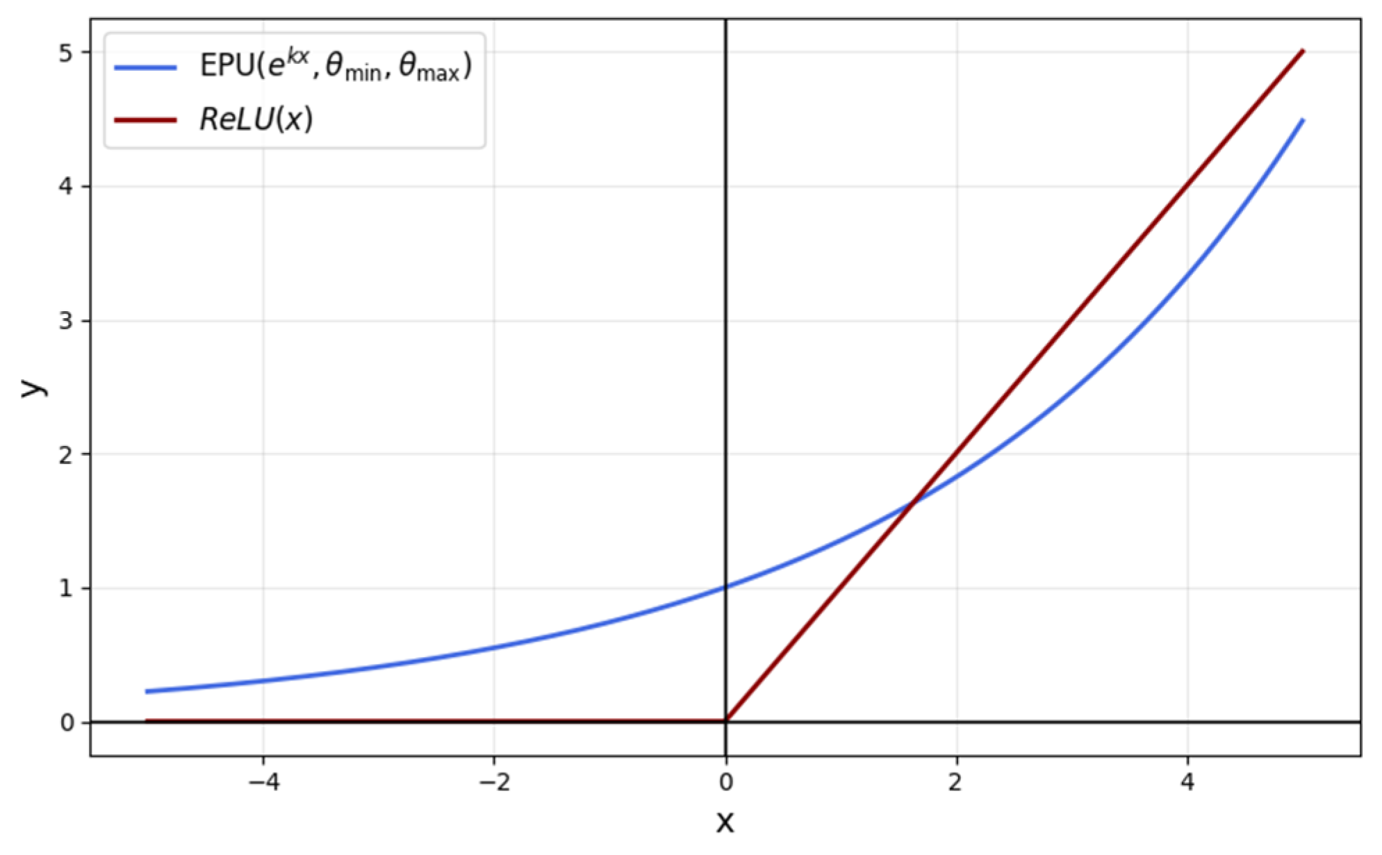
This paper presents a new activation function called Exponential Partial Unit (EPU), which is based on the exponential function. Although it does not belong to the ReLU family, it combines low computational complexity and greater flexibility with respect to real data. The formula that describes the EPU is as follows:

$$\mathrm{EPU}\left(\mathrm{x}\right)=\mathrm{clip}\left(e^{kx},{\mathsf{\theta }}_{\min },{\mathsf{\theta }}_{\max }\right)$$

(4)

where $e^{kx}$ represents the exponential function with base e raised to the power of the scaling factor k times the input variable. ${\theta }_{min} \mathrm{a}\mathrm{n}\mathrm{d} {\theta }_{max}$ represent the minimum and maximum bounds, respectively. The clip function is defined as

$$clip(e^{kx}, {\theta }_{min}, {\theta }_{max})=\left\{\begin{array}{c}{\theta }_{min}, if e^{kx}<{\theta }_{min} \\ e^{kx}, if {\theta }_{min}<e^{kx}<{\theta }_{max}\\ {\theta }_{max}, if e^{kx}>{\theta }_{max} \end{array}\right.$$

(5)

In the proposed function, the parameters k, ${\theta }_{min} \mathrm{a}\mathrm{n}\mathrm{d} {\theta }_{max}$ are defined as learnable parameters, allowing them to be dynamically optimized during the training process, all initialized following uniform distribution. The boundary of initialization of these parameters differs from each other. The parameter min is initialized within a negative range, ensuring that it acts as a lower bound when clamping input values, between −5 and −1.

$${\mathsf{\theta }}_{min}\sim \mathcal{U}\left(-\mathrm{5,1}\right)$$

(6)

Symmetrically, ${\theta }_{max}$ is initialized within a positive range from 1 to 5. By enforcing ${\theta }_{min}$< ${\theta }_{max}$ at initialization, the function ensures a well-defined input transformation.

$${\mathsf{\theta }}_{max}\sim \mathcal{U}\left(\mathrm{1,5}\right)$$

(7)

Meanwhile, k is initialized within a small positive range, controlling the scaling factor in the exponential function.

$$k\sim \mathcal{U}\left(\mathrm{0,1}\right)$$

(8)

Figure 1 illustrates the comparison between the ReLU and EPU functions, highlighting their respective behaviors across the specified range.

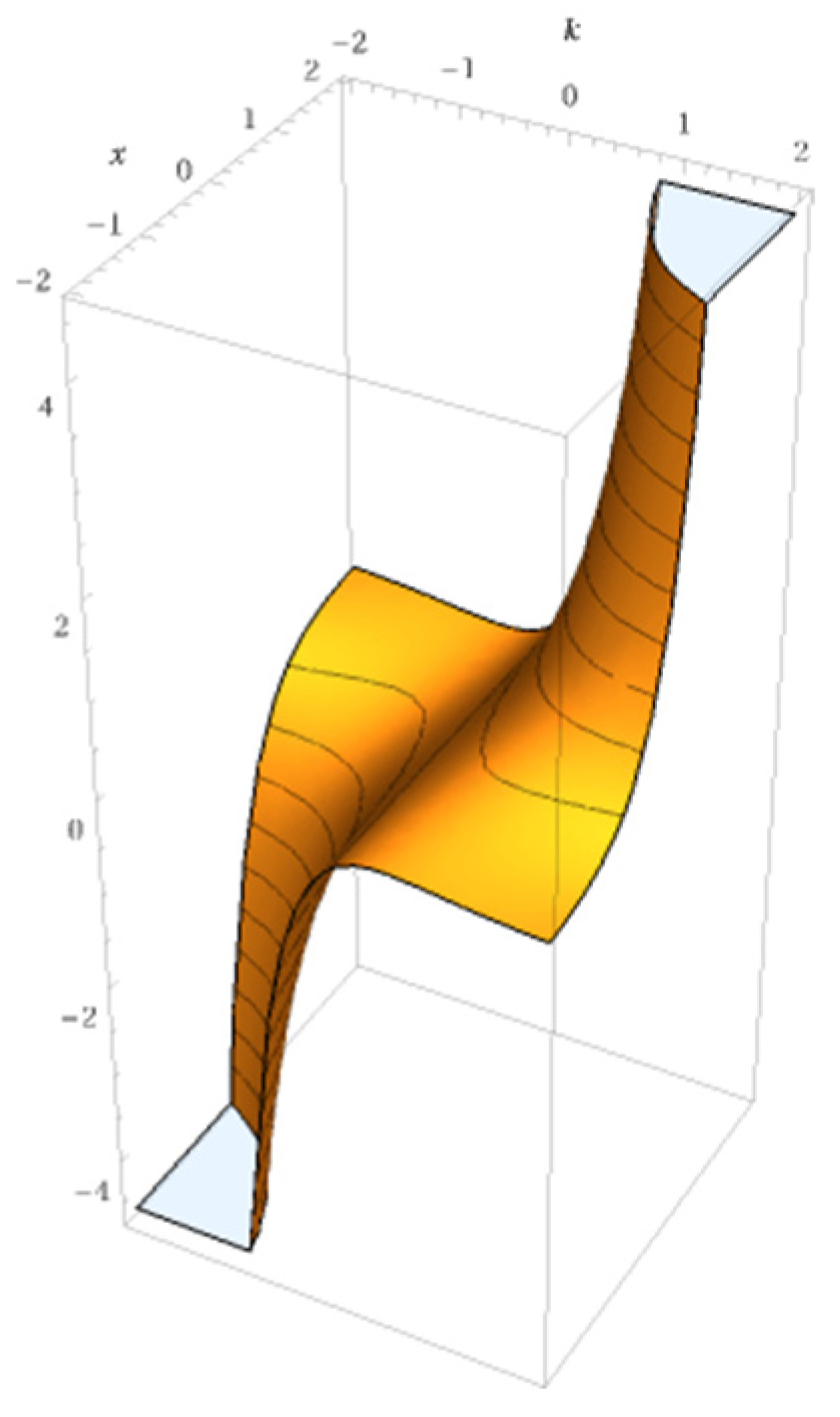
One of the major advantages of the EPU is its ability to introduce non-linearity while maintaining smooth gradient flow, which enhances optimization and helps prevent “vanishing gradients”. Another advantage is that its first derivative can be easily calculated during training. This property simplifies the backpropagation process, as the gradient of the activation function can be efficiently computed, ensuring smooth and stable updates to the learnable parameters. The derivative of the exponential function is straightforward, making it computationally efficient for optimization tasks, and it helps maintain the stability of the training process. The 3D plot is shown in Figure 2, providing a visual representation of the function's behavior.

$${\displaystyle \frac{d}{dx}}\left(e^{kx}\right)=k{e}^{kx}$$

(9)

We acknowledge the extensive development of ReLU variants, each designed to address specific limitations of the original ReLU function. While these variants generally introduce only minor modifications to the core ReLU concept, they nonetheless offer measurable improvements in aspects like mitigating the vanishing gradient problem, accelerating convergence, or enhancing the performance of certain tasks.

In contrast, our proposed activation function presents a novel approach that distinguishes itself from the traditional ReLU family. By uniquely integrating the exponential function in a way that fundamentally redefines activation behavior, our method offers an innovative alternative that not only addresses existing limitations, but also introduces distinct performance benefits and enhanced stability. This new concept goes beyond incremental modifications, representing a significant and original contribution to the design of activation functions.

In modern deep learning frameworks, neural networks rely heavily on automatic differentiation to efficiently compute gradients during training. This capability is particularly important when employing novel activation functions like our Exponential Partial Unit (EPU). Thanks to the straightforward derivative of the exponential function our EPU enables faster, and more efficient gradient computation compared to more complex activation functions. This computational efficiency not only accelerates the automatic differentiation process, but also contributes to faster overall training and enhanced stability during backpropagation.

Furthermore, as noted in [22,23], the existing literature does not provide a detailed analysis of activation functions that employ such an exponential integration approach. This highlights the novelty of our method, which extends beyond traditional modifications of ReLU and offers a unique contribution to activation function design.

3.2. Batch Normalization

Generally, in neural networks, the output of the first layer is used as input to the second layer, the output of the second layer is fed to the third layer, and this process continues on. When the parameters of a layer are changed during training, this results in a change in the distribution of input values for subsequent layers. These input distribution changes can lead to serious complications, especially if the network has more layers. This problem is described in detail in [24], as follows: “We define Internal Covariate Shift as the change in the distribution of network activations due to the change in network parameters during training”. This problem is solved precisely by Batch Normalization. Other normalization approaches have appeared as well, such as Group Normalization [25] and Switchable Normalization [26], but for the experiments in this study, we have decided to use Batch Normalization due to its popularity and good benchmark results.

For a given mini-batch of input data, the mean and variance are first computed.

$${\mathsf{\mu }}_B={\displaystyle \frac{1}{m}}\sum _{i=1}^m{x}_i$$

(10)

$${\mathsf{\sigma }}_B^2={\displaystyle \frac{1}{m}}\sum _{i=1}^m{\left(x_i-{\mathsf{\mu }}_B\right)}^2$$

(11)

Then, this “normalization” is applied to each input x by subtracting the mean ${\mu }_B$ and dividing by the square root of the variance ${\sigma }_B^2$, with a small constant ϵ added to the denominator to prevent division by zero and ensure numerical stability.

$$\widehat{x_i}={\displaystyle \frac{x_i-{\mathsf{\mu }}_B}{\sqrt{{\mathsf{\sigma }}_B^2+\mathsf{ϵ}}}}$$

(12)

After normalization, the data are scaled and shifted using learnable parameters γ and β These parameters, which are optimized during training, allow the network to retain or adapt an optimal representation of the data after normalization.

$$y_i=\mathsf{\gamma }\widehat{x_i}+\mathsf{\beta }$$

(13)

3.3. Regularization

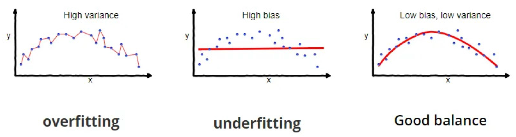
Oversaturation has always plagued neural network designers. Ordinary users would never realize how much time and effort is required for solving high-variance problems. High variance and high bias are two major components of prediction error. A high-variance model pays too much attention to the training data and fails to perform well on new, unseen data. This can lead to very high scores on the training data, but low scores on validation and tests. On the other hand, a high-bias model pays too little attention to the training data and makes overly simplistic inferences that do not reflect the complexity of the problem well. This leads to large errors in all data distributions. These two types of errors—variance and bias—create a tradeoff called the bias–variance tradeoff, shown in Figure 3. When we try to reduce one error, it often leads to an increase in the other. To find the perfect balance, various regularization methods have emerged. Among the most well-known methods are L2 regularization [27] and Dropout [28]. As presented in [29], L2 shows better results in some cases, while Dropout works better in others. To address the bias–variance tradeoff effectively, we use both methods in this study.

The idea behind Dropout is simple: During training some neurons are “turned off’’. At each training step, a random subset of neurons in a layer is selected and temporarily deactivated. These neurons do not contribute to either forward propagation or backpropagation during that step. By deactivating neurons at random, the network is forced to rely on a wider range of neurons rather than depending too much on specific ones. This encourages the model to learn more robust and diverse patterns from the data, making it better at handling new, unseen examples.

The dropout rate is a hyperparameter that determines the probability of a neuron being dropped. For instance, a dropout rate of 0.2 means that 20% of neurons will be deactivated at each training step. Sometimes, an improperly chosen dropout rate can significantly impact the effectiveness of training, potentially deteriorating the model’s performance. To compensate for the absence of the dropped neurons, the outputs of the remaining active neurons are scaled up. For instance, if 50% of neurons are deactivated, the outputs of the remaining active neurons are scaled up by a factor equal to the probability of keeping a neuron active. This helps maintain the network’s overall functionality and balance during training. During testing, dropout is turned off. All neurons are active, but their weights are adjusted to match the expected behavior during training. In our study, wherever dropout is used, the dropout rate is set to 0.2.

Besides Dropout, as mentioned earlier, another method of regularization is used—L2 Regularization also known as Weight Decay. In our case, we limit the complexity of the model with this method by limiting the update of the weights. This function takes away from the complexity of the model by adding the element called the regularization term. The regularization term is added to the underlying cost function, thus affecting the optimization process. The standard cost function J(W), which measures the difference between predicted and actual output values, can be extended by adding the L2 regularization. Thus, the cost function becomes

$$J={\displaystyle \frac{1}{m}}\sum _{i=1}^m\mathcal{L}\left(\widehat{y_i},y_i\right)+{\displaystyle \frac{\mathsf{\lambda }}{2m}}\sum _{l=1}^L|w^{\left[l\right]}{|}_2^2$$

(14)

This addition to the cost function results in smaller weights, which in turn reduces the ability of the model to overfit to specific examples in the training data. λ is a regularization hyperparameter that controls the balance between the model’s accuracy on the training data and its complexity. m is the number of training examples used to train the model, and L is the loss function that computes the difference between the predicted value $\widehat{y}$ and the actual value y for each training example i. ${\left|w^{\left[l\right]}\right|}_2^2$ represents the L2-norm of the weights of layer l, that is, the sum of the squares of all the elements of the weights.

$$|w^{\left[l\right]}{|}_2=\sqrt{\sum _{i=1}^{n_l}\sum _{j=1}^{n_{l-1}}{\left(w_{ij}^{\left[l\right]}\right)}^2}$$

(15)

Once we compute the gradients of the cost function with an added regularization term, the weight update is

$$dW\left[l\right]={\displaystyle \frac{\partial \mathcal{L}}{\partial W\left[l\right]}}+{\displaystyle \frac{\mathsf{\lambda }}{m}}W\left[l\right]$$

(16)

3.4. He Initialization

Initialization in neural networks is the process of setting the initial values of the weights before training. This step is the key in creating models with fast convergence. Poorly initialized weights can slow down training or even make it impossible. Typically, these weights are initialized by following some distribution (most commonly a normal or uniform distribution) [30]. However, there are other methods that are based on activation functions. For example, Xavier Initialization [31] is designed for functions such as sigmoid and tanh, guaranteeing similarity of variance of inputs and outputs.

This paper considers another initialization approach, He Initialization [20], which we empirically found to be the most appropriate in our case. After all, this method was designed to improve the performance of image recognition architectures. The main idea behind He Initialization is to ensure that the variance of the outputs from each layer of the network remains almost unchanged when passing through a layer. This helps prevent excessive increase or decrease in gradients during training, which can lead to faster convergence and better model performance.

$$W\sim \mathcal{N}\left(0,{\displaystyle \frac{2}{n_{\mathrm{in}}}}\right)$$

(17)

This formula describes the He initialization of the weights in the neural network, where the weights are initialized with a normal distribution with zero mean and variance proportional to two, divided by the number of inputs to the layer n_in. This method ensures the stability of the gradients and prevents the problems of decay or explosion of the gradients when using activation functions such as ReLU and, in our case, EPU.

3.5. The Neural Network

Deep neural networks are a foundational approach in artificial intelligence (AI) to solve different types of problems in a robust manner. They are the basis of popular architectures such as transformer [32], which in turn underlie modern chatbots and solutions for natural language processing (NLP) tasks. In computer vision, architectures such as Vision Transformer (ViT) [33], built on the principles of the previously mentioned transformers, find applications in tasks such as image classification, object detection, and segmentation. Other models, such as U-Net [34], specialize in semantic and medical segmentation tasks, making them widely used in medical diagnostics. These neural networks can be of different types—feed-forward neural networks (FFNNs), convolutional neural networks (CNNs), recurrent neural networks (RNNs), as well as specialized architectures such as graph neural networks (GNNs) and autoencoders for specific tasks.

One of the first approaches to solving the image classification problem considered in this paper is using a FFNN. Ever since the distant past [35] until now [36], people have been trying to develop models that can efficiently process and classify visual data using FFNNs. Although FFNNs can be used for tasks such as image classification, it has its limitations, especially when it comes to processing high-resolution images or large amounts of data. This is due to the fact that FFNN does not take into account the scale structure of the images. One of the main problems in using this type of networks for image classification is related to the size of the input data. Images are usually represented as matrices of pixels, and in order to be processed by FFNNs, these matrices need to be transformed into long vectors. For high-resolution images, this leads to increased computational complexity, memory requirements, and the risk of overtraining. Other serious issues are spatial locality and translational invariance. Spatial locality means that the pixels that form an object are located close to each other, but FFNNs treat each pixel as independent, ignoring these dependencies and losing important information about the structure of the object. Translational invariance assumes that objects remain identical even if they are shifted in the image, but FFNNs do not recognize such shifts, requiring retraining for each new position. These limitations lead to an extremely large number of parameters and inefficiency in classifying more complex images. This is when CNNs (convolutional neural networks) came along and revolutionized image processing. The first successful model of this kind was LeNet [37], which laid the foundation for all modern image recognition models. Convolution in CNNs refers to processing the input image with a series of filters. Using these filters, instead of treating pixels as isolated points, CNNs use connection layers (convolutional layers) that analyze small regions of the image (called receptive fields). This allows the extraction of local features such as edges, textures, and shapes. CNNs also use pooling operations that aggregate information into small areas and allow the network to recognize objects regardless of their exact location in the image. Another important aspect, which is also a major theme of this paper, is that, thanks to these filters, the parameters in such networks are significantly smaller compared to traditional FFNNs.

3.6. The Proposed Architecture

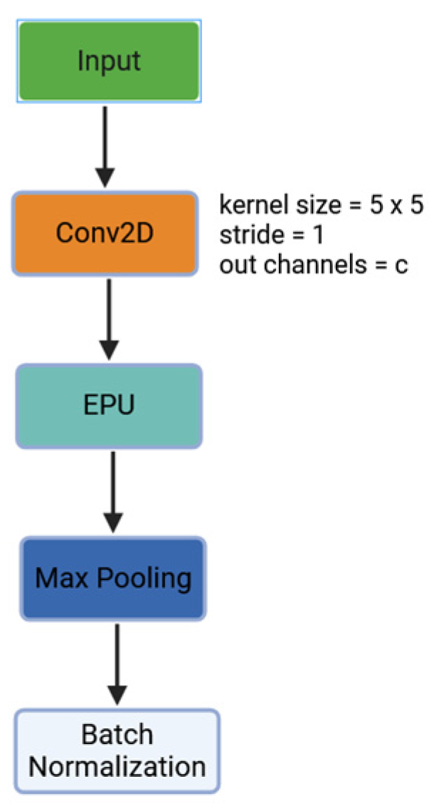
In this subsection, we present our CNN structure, which contains only three convolutional layers, one fully connected layer, and the output layer. Each convolutional layer follows the same structure, which we refer to as a ConvBlock, visualized in Figure 4.

As already mentioned, the input image is presented in a two-dimensional format with a size of 32 × 32 pixels. Each pixel contains information for three color channels (R, G, and B), with 8 bits allocated for each channel, for a total of 24 bits per pixel. We will write the input information to the first ConvBlock for processing as a tensor with dimensions 32 × 32 × 3.

The information is first processed through a convolutional layer (filter) that is configured with a kernel size of 5, a stride equal to 1, and padding set to “same”. This configuration preserves the spatial dimensions of the image. The output of this layer consists of a c number of (color) channels, which determines the number of features that will be extracted from the input image. After performing the convolution, the output, organized into a tensor with dimensions (h, w, and c)–with h and w representing the spatial dimensions–is fed directly to the proposed activation function EPU for further processing. After convolution, the data are subjected to pooling, specifically max pooling, which is applied with kernel size 2 and stride 2. This reduces the spatial dimensions significantly, which helps to lower the computational complexity and eliminate redundant information while preserving the most important features for the subsequent processing steps. After the convolution and merging operations are completed, the data undergo Batch Normalization. This process normalizes the values in the tensor with respect to the mean and standard deviation, as previously described by Formulas (1)–(3).

The whole network has a total of three such ConvBlocks. After being processed, the input information (image) of size (32 × 32 × 3) is resized to (4 × 4 × 64), where 64 is the value of c, for the last ConvBlock. This final tensor is considered a feature vector which contains (4 × 4 × 64), 1024 elements in total. Each element of this vector represents a numerical feature extracted from the input image that summarizes its essence and is ready for further processing by the fully connected layer and the output layer of the network. This feature vector is the input to the fully connected layer containing 128 hidden units, this time followed by ReLU activation function instead of EPU. The output from the fully connected layer then goes to the output layer of the network, which is again FF, but this time with only 10 hidden units because that is the number of classes in the dataset. In order to make a prediction, the output from the output layer goes through a softmax activation function that looks like this:

$$\mathrm{softmax}\left(x_i\right)={\displaystyle \frac{e^{x_i}}{{\sum }_{j=1}^n{e}^{x_j}}}$$

(18)

It provides the probability for each class. The class with the highest probability is set as the final answer.

3.7. Parameters

As presented in Section 2, the number of parameters required to achieve similar levels of accuracy has been significantly reduced. By optimizing the number of learnable parameters, this architecture can achieve a performance that is comparable to the most advanced models in the field, while being much more efficient. The number of learnable parameters in the three convolutional layers within each ConvBlock has been reduced to a minimal value. The number of a convolutional layer is calculated using the following formula:

$$P_{\mathrm{conv}}=\left(F_h\times F_w\times C_{\mathrm{in}}\times C_{\mathrm{out}}\right)+C_{\mathrm{out}}$$

(19)

In this formula F_h and F_w are the height and width of the kernel, while C_in, C_out correspond to the input and output channels, respectively. The term C_out is added to account for the bias parameters, with one bias per output channel.

This formula helps in determining the number of parameters needed for each convolutional layer, considering factors like the size of the filter, the number of filters, and the input and output dimensions.

In addition to the convolutional layers, the Batch Normalization layers and the proposed activation function EPU are also parameter-dependent in ConvBlock. The Batch Normalization layer adds two learnable parameters per channel (mean and standard deviation), while EPU includes three additional learnable parameters. This is the result of the way they are configured. Therefore, the total number of parameters in a ConvBlock is the sum of the parameters of all convolutional layers, the parameters from Batch Normalization and the parameters from the activation function:

$$P_{\mathrm{total}}=P_{\mathrm{conv}}+P_{\mathrm{EPU}}+P_{\mathrm{BN}}$$

(20)

In turn, in a fully connected neural network (FFNN), the number of parameters depends on the number of neurons in each layer and the connections between them. Each layer contains two types of learnable parameters: weights and biases. The weights define the strength of the connections between neurons in different layers, while the biases adjust the output of each neuron to improve the model’s ability to fit the data. The number of weight parameters for a certain layer in an FFNN is calculated as follows:

$${\mathrm{W}}_{\mathrm{l}}\mathrm{ }=\mathrm{ }{\mathrm{N}}_{\mathrm{i}\mathrm{n}}\mathrm{ }\times {\mathrm{N}}_{\mathrm{o}\mathrm{u}\mathrm{t}}$$

(21)

where $N_{in}$ and $N_{out}$ are the number of neurons in the past and previous layer, respectively. The number of bias parameters for a layer is equal to the number of neurons in that layer, as each neuron has one associated bias parameter. Therefore, the number of bias parameters for a layer is

$$B_l=N_{out}$$

(22)

The total number of parameters, for a layer is

$$P_l=\left(N_{in}\times N_{out}\right)+N_{out}$$

(23)

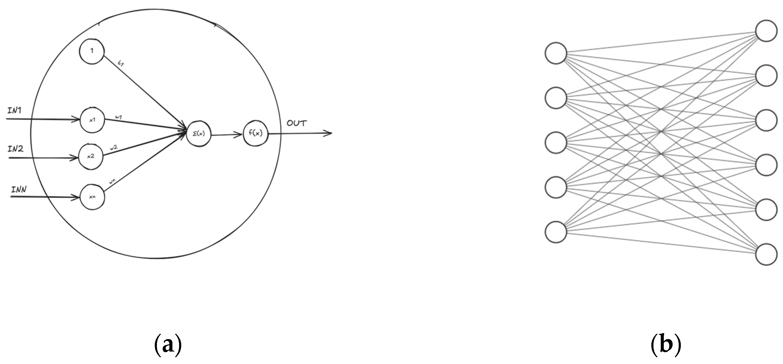
Figure 5a illustrates the architecture of a classical perceptron or one (hidden) unit, where IN1 to INn represent the input nodes, w1 to wn correspond to the associated weights, and b1 denotes the bias term. Σ(x) represents the summation function, while f(x) is the activation function that introduces non-linearity.

For example, Figure 5b considers a connection between two layers where the first layer contains five hidden units and the second layer contains six. The total number of parameters would be calculated as 5 × 6 + 6 = 36, accounting for both the weights and biases. In our particular case, the system has two of these connections, as previously mentioned.

The first connection in our network has an input dimensionality (Nin) of 1024 and an output dimensionality (Nout) of 128. The second connection then takes this 128-dimensional feature representation as its input (Nin = 128) and maps it to an output of size 10 (Nout = 10), corresponding to the number of distinct classes in our dataset.

As shown in

Table 1. Number of parameters in our proposed architecture’s network blocks.

Block Type	Number of Parameters
ConvBlock1	1221
ConvBlock2	12,837
ConvBlock3	51,269
FFNN1	131,202
FFNN2	1290
Total:	197,819

, the number of parameters in our proposed architecture’s network blocks is as follows:

4. Training and Results

4.1. Hardware and Software of the Platform

The neural network training was conducted on a single NVIDIA GeForce RTX 3080 (12GB VRAM) GPU (Most Computers, Sofia, Bulgaria), which provided significant computational power for handling deep learning workloads efficiently. We trained the system using PyTorch version 2.4, taking advantage of its optimized support for CUDA acceleration, automatic mixed-precision training, and efficient tensor operations.

CUDA Cores are parallel processors inside NVIDIA GPUs that handle multiple tasks simultaneously. They function similarly to CPU cores but are optimized for high-throughput computations, making them ideal for deep learning, gaming, and computing. In the case of the NVIDIA RTX 3080 (12 GB), there are 8960 CUDA Cores, meaning it can perform thousands of matrix multiplications and tensor operations at once—key processes in training deep neural networks.

With 8960 CUDA Cores, the RTX 3080 provides excellent performance for both model training and inference. However, newer GPUs, such as the RTX 4090 and enterprise-grade options like the NVIDIA H100, offer significantly improved performance, higher memory capacity, and better efficiency for large-scale deep learning workloads.

4.2. Training

The model was trained for 1000 epochs using backpropagation and the Adam optimizer. Because the CNN architecture is relatively simple—with fewer layers and parameters—it requires more epochs for the model to learn the intricate patterns in the data. However, each epoch only takes around 2000 milliseconds due to the lightweight design. In contrast, more complex models, like deeper networks with residual connections (e.g., ResNet), have a higher per-epoch computational cost because they process a larger number of parameters and more layers. Thus, while those models might converge in fewer epochs, each epoch could take several seconds, leading to a longer overall training time. This tradeoff between model complexity and training duration highlights the efficiency of our simpler architecture in terms of computational resource usage per epoch.

As shown in Figure 6 and Figure 7, given that the loss continued to decrease throughout the 1000 epochs, it suggests that further training beyond 1000 epochs could potentially yield even better results. The gradual improvement seen in the training process indicates that the model has not yet fully converged and there is still room for improvement.

4.3. Results

The model achieved a training accuracy of 77.2% and a test accuracy of 81.6%, demonstrating its ability to learn relevant features effectively from the CIFAR-10 dataset. Both the training and testing losses continued to decrease steadily, indicating that the model was effectively optimizing during the training phase. Similarly, the test loss followed a downward trend, suggesting good generalization to unseen data.

Execution time refers to the duration a program or algorithm takes to complete a task on a given hardware system. It is a crucial factor in evaluating performance, efficiency, and scalability.

In our case, the preprocessing of a single image takes 0.43 milliseconds (ms). This measurement serves as a baseline for performance evaluation and allows us to compare different implementations or optimizations.

As shown in Figure 8, the accuracy continues to improve as the epochs increase. In that case, we refer to the accuracy as Top-1 accuracy. Top-K accuracy is an evaluation metric in machine learning that indicates whether the correct class is present within the top K predictions. The most commonly used Top-K accuracies are Top-1, Top-3, and Top-5, with their corresponding results presented in

Table 2. Top-K accuracies on CIFAR-10 for 1000 epochs.

Top-K	Accuracy (%)
Top-1	81.6
Top-3	95.97
Top-5	98.87

. These Top-K accuracy metrics provide a more comprehensive understanding of a model’s performance, especially in scenarios where the correct class might not always be the top prediction. Top-1 accuracy focuses on the exact match, while Top-3 and Top-5 accuracies allow for a more lenient evaluation by considering the presence of the correct class among the top three or top five predictions, respectively. In our case both Top-3 and Top-5 accuracies have nearly perfect predictions, because of the small dataset. Even though the dataset is small, the high Top-3 and Top-5 accuracies are still a positive outcome, indicating that the model is performing well in predicting the correct classes within its top predictions.

4.4. Understanding the Model’s Learned Representations

After the training, the model learns to represent images as points in a high-dimensional vector space, where similar images are mapped to nearby points. This approach is usually used in the context of natural language processing (NLP) for word embeddings, first introduced in [38]. The approach is really suitable for computer vision as well, because by mapping images to vectors, we can better understand and visualize what the model has learned during training. In our case, the image vectors are derived from the final layer of our network, which has a size of 128, providing a compact yet informative representation of each image. Word embeddings and image embeddings are commonly used in security applications such as anomaly detection, facial recognition, and identifying fraudulent activities by comparing patterns in large datasets.

As shown in Figure 9 the visualization of the 2D projection of learned image embeddings is obtained using principal component analysis (PCA).

Some misclassifications, shown in Figure 10, are understandable even for human observers, such as a deer being mistaken for a horse or an automobile for a truck. These errors highlight the inherent difficulty in distinguishing visually similar classes, emphasizing the complexity of image classification tasks.

4.5. Assessing Model Generalization: A Comparative Analysis Across Activation Functions

To evaluate the overall generality of our architecture, we train the model on both CIFAR-10 and CINIC-10. In addition, we compare several popular activation functions—such as ReLU, Leaky ReLU, and ELU—with our proposed activation function, EPU.

By incorporating CINIC-10, a dataset known for its increased diversity and complexity relative to CIFAR-10, we aim to examine how well the model generalizes across different data distributions. The comparative analysis focuses on assessing the impact of each activation function on the model’s performance and generalization capabilities. Specifically, we analyze whether our proposed EPU function can yield improvements over traditional activation functions by facilitating more robust feature learning and reducing the generalization gap between training and test performance.

This comprehensive evaluation will help us understand the interplay between dataset complexity, network architecture, and activation function choice, and ultimately guide the development of models that perform reliably in real-world scenarios.

Table 3. Top-1 accuracies on CIFAR-10 for 250 epochs.

Activation Function	Accuracy (%)
EPU	78.32
ReLU	78.77
LeakyReLU	79.3
ELU	79.47

provides the top-1 accuracies on the CIFAR-10 dataset after training for 250 epochs.

Figure 11 illustrates the test accuracy for different activation functions on the CIFAR-10 dataset. This figure compares the performance of various activation functions, providing insight into their impact on the overall accuracy of the model.

It can be observed that our proposed function, EPU, initially performs slightly worse than the other activation functions. This is due to the fact that CIFAR-10 contains very few images (i.e., it is a small dataset), and since EPU is fine-tuned during training, achieving its best performance requires either more images or more training iterations.

These arguments become evident when training on CINIC-10, a dataset that is several times larger than CIFAR-10. With CINIC-10, while the performance of all activation functions tends to decline—likely due to model saturation—the model using EPU continues to improve steadily and achieves the highest accuracy percentage, as shown in both

Table 4. Top-1 accuracies on CINIC-10 for 250 epochs.

Activation Function	Accuracy (%)
EPU	65.88
ReLU	65.2
LeakyReLU	65.5
ELU	65.42

and Figure 12.

This outcome not only highlights the scalability of the EPU function with larger datasets but also underscores the importance of adequate data volume and sufficient training iterations for adaptive activation functions. Further experiments with even larger datasets or extended training periods could potentially demonstrate additional advantages of EPU over conventional activation functions.

4.6. Floating Point Operations per Second (FLOPs)

Floating Point Operations per Second (FLOPs) is a metric that quantifies the number of floating-point calculations a computer system can perform in one second. Floating-point operations involve arithmetic calculations—such as addition, subtraction, multiplication, and division—on real numbers represented in a format that can accommodate a wide range of values. This capability is essential for applications requiring high precision and handling of very large or very small numbers.

Table 5. FLOPs for every activation function model.

Activation Function	FLOPs (NMac)
EPU	8.02
ReLU	8.07
LeakyReLU	8.04
ELU	8.07

shows that models employing the EPU activation function require fewer FLOPs (8.02 NMac) compared to those using ReLU (8.07 NMac), LeakyReLU (8.04 NMac), and ELU (8.07 NMac). This suggests that EPU is the most computationally efficient among the compared activation functions.

While the differences in FLOPs presented in this table may seem minimal, they can become significant when processing large-scale images or deploying models in resource-constrained environments. In such scenarios, even slight reductions in computational requirements per operation can lead to substantial savings in processing time and energy consumption. Therefore, adopting the EPU activation function could enhance the efficiency and scalability of models, particularly in applications involving high-resolution images or large datasets.

Table 6. Performance metrics of the EPU model versus state-of-the-art models.

Activation Function	FLOPs (NMac)	Number of Parameters
EPU model	8.02	197.8 k
ResNet-18	37.75	11.69 M
EfficientNet-b0	10.25	5.29 M
VGG-11	277.13	132.86 M

presents a comparative analysis of the EPU model’s performance metrics alongside several state-of-the-art convolutional neural networks (CNNs): ResNet-18, EfficientNet-B0, and VGG-11. The comparison focuses on two critical aspects: Floating Point Operations (FLOPs) and the number of parameters, providing insight into both the computational efficiency and model complexity.

5. Conclusions and Future Work

5.1. Conclusions

The presented system is lightweight and convenient to use on any device thanks to its efficient architecture and well-optimized learning algorithms. Despite its simplicity, the network achieves results comparable to those of leading models. This makes it suitable for a variety of applications that require fast image processing and real-time classification, such as driving cameras, web security, and various aspects of cybersecurity. In the context of cybersecurity, the system has the potential to be used in multiple critical scenarios, especially in automated threat detection in network traffic, according to the type of input formatting, and video stream analysis for real-time detection of suspicious activities, on devices ranging from small IoT systems to larger infrastructures. In addition, the system offers flexibility and adaptability, making it suitable for integration into existing infrastructures without the need for significant hardware or software changes. This is particularly important in the cybersecurity domain, where rapid response to new threats is essential. The ability to operate in real-time, combined with low resource requirements, makes the system ideal for deployment in scalable environments, such as large enterprise networks or even IoT devices. Also, its ease of use and high performance make it accessible to a wide range of users, from small enterprises to large organizations looking for effective security and data analytics solutions.

Nevertheless, our system still falls short of the performance achieved by state-of-the-art models. Those advanced models are typically pre-trained on vast and diverse datasets like ImageNet, which allow them to learn intricate patterns that simply cannot be captured from a smaller dataset such as CIFAR-10 alone. In our case, the hardware limitations prevent us from pre-training on a large-scale dataset like ImageNet before fine-tuning on CIFAR-10, making a direct comparison between our model and these pre-trained giants somewhat unfair.

5.2. Future Work

We can try to optimize the system by making a reasonable tradeoff between the number of parameters, accuracy, and execution time. We can also factor into the equation factors such as the memory required for running the system and its energy efficiency. Additionally, investigating advanced data augmentation techniques may further improve performance by enriching the diversity of the training data and reducing overfitting.

In parallel, the newly discovered activation function EPU, which has already demonstrated better performance in computer vision compared to its predecessors, could be the subject of future research. It has the potential to show equally good results in natural language processing (NLP) tasks, such as the use of transformers, and in reinforcement learning environments. Moreover, our activation function could be incorporated in studies like [39], where similar architectural optimizations are explored, to further validate its applicability across diverse domains.

References

1. Krizhevsky, A.; Sutskever, I.; Hinton, G.E. ImageNet classification with deep convolutional neural networks. Commun. ACM 2017, 60, 84–90. [Google Scholar] [CrossRef]
2. Szegedy, C.; Liu, W.; Jia, Y.; Sermanet, P.; Reed, S.; Anguelov, D.; Erhan, D.; Vanhoucke, V.; Rabinovich, A. Going Deeper with Convolutions. arXiv 2014, arXiv:1409.4842. [Google Scholar] [CrossRef]
3. He, K.; Zhang, X.; Ren, S.; Sun, J. Deep Residual Learning for Image Recognition. arXiv 2015, arXiv:1512.03385. [Google Scholar] [CrossRef]
4. Deng, J.; Dong, W.; Socher, R.; Li, L.-J.; Li, K.; Li, F.-F. ImageNet: A large-scale hierarchical image database. In Proceedings of the 2009 IEEE Conference on Computer Vision and Pattern Recognition, Miami, FL, USA, 20–25 June 2009; IEEE: New York, NY, USA, 2009; pp. 248–255. [Google Scholar]
5. Coates, A.; Lee, H.; Ng, A.Y. An Analysis of Single-Layer Networks in Unsupervised Feature Learning. In Proceedings of the Fourteenth International Conference on Artificial Intelligence and Statistics, Fort Lauderdale, FL, USA, 11–13 April 2011. [Google Scholar]
6. Li, F.-F.; Fergus, R.; Perona, P. Learning Generative Visual Models from Few Training Examples: An Incremental Bayesian Approach Tested on 101 Object Categories. In Proceedings of the 2004 Conference on Computer Vision and Pattern Recognition Workshop, Washington, DC, USA, 27 June–2 July 2004; IEEE: New York, NY, USA, 2004; p. 178. [Google Scholar]
7. LeCun, Y.; Cortes, C.; Burges, C.J.C. The MNIST Database of Handwritten Digits. Available online: http://yann.lecun.com/exdb/mnist (accessed on 10 April 2025).
8. Krizhevsky, A. Learning Multiple Layers of Features from Tiny Images. Master’s Thesis, University of Tront, Toronto, ON, Canada, 2009. [Google Scholar]
9. Darlow, L.N.; Crowley, E.J.; Antoniou, A.; Storkey, A.J. CINIC-10 is not ImageNet or CIFAR-10. arXiv 2018, arXiv:1810.03505. [Google Scholar] [CrossRef]
10. Doon, R.; Kumar Rawat, T.; Gautam, S. Cifar-10 Classification using Deep Convolutional Neural Network. In Proceedings of the 2018 IEEE Punecon, Pune, India, 30 November–2 December 2018; IEEE: New York, NY, USA, 2018; pp. 1–5. [Google Scholar]
11. Visin, F.; Kastner, K.; Cho, K.; Matteucci, M.; Courville, A.; Bengio, Y. ReNet: A Recurrent Neural Network Based Alternative to Convolutional Networks. arXiv 2015, arXiv:1505.00393. [Google Scholar] [CrossRef]
12. Calik, R.C.; Demirci, M.F. Cifar-10 Image Classification with Convolutional Neural Networks for Embedded Systems. In Proceedings of the 2018 IEEE/ACS 15th International Conference on Computer Systems and Applications (AICCSA), Aqaba, Jordan, 28 October–1 November 2018; IEEE: New York, NY, USA, 2018; pp. 1–2. [Google Scholar]
13. Ge, R.; Feng, X.; Song, S.; Chang, H.-C.; Li, D.; Cameron, K.W. PowerPack: Energy Profiling and Analysis of High-Performance Systems and Applications. IEEE Trans. Parallel Distrib. Syst. 2010, 21, 658–671. [Google Scholar] [CrossRef]
14. Iandola, F.N.; Han, S.; Moskewicz, M.W.; Ashraf, K.; Dally, W.J.; Keutzer, K. SqueezeNet: AlexNet-level accuracy with 50x fewer parameters and <0.5MB model size. arXiv 2016, arXiv:1602.07360. [Google Scholar] [CrossRef]
15. Pathak, D.; El-Sharkawy, M. ReducedSqNet: A Shallow Architecture for CIFAR-10. In Proceedings of the 2018 International Conference on Computational Science and Computational Intelligence (CSCI), Las Vegas, NV, USA, 13–15 December 2018; IEEE: New York, NY, USA, 2018; pp. 380–385. [Google Scholar]
16. Nair, V.; Hinton, G.E. Rectified Linear Units Improve Restricted Boltzmann Machines. In Proceedings of the 27th International Conference on Machine Learning (ICML-10), Haifa, Israel, 21–24 June 2010. [Google Scholar]
17. Maas, A.L.; Hannun, A.Y.; Ng, A.Y. Rectifier Nonlinearities Improve Neural Network Acoustic Models. In Proceedings of the 30th International Conference on Machine Learning, Atlanta, GA, USA, 16–21 June 2013. [Google Scholar]
18. Clevert, D.-A.; Unterthiner, T.; Hochreiter, S. Fast and Accurate Deep Network Learning by Exponential Linear Units (ELUs). arXiv 2016, arXiv:1511.07289. [Google Scholar] [CrossRef]
19. Klambauer, G.; Unterthiner, T.; Mayr, A.; Hochreiter, S. Self-Normalizing Neural Networks. arXiv 2017, arXiv:1706.02515. [Google Scholar] [CrossRef]
20. He, K.; Zhang, X.; Ren, S.; Sun, J. Delving Deep into Rectifiers: Surpassing Human-Level Performance on ImageNet Classification. arXiv 2015, arXiv:1502.01852. [Google Scholar] [CrossRef]
21. Maniatopoulos, A.; Mitianoudis, N. Learnable Leaky ReLU (LeLeLU): An Alternative Accuracy-Optimized Activation Function. Information 2021, 12, 513. [Google Scholar] [CrossRef]
22. Mahima, R.; Maheswari, M.; Roshana, S.; Priyanka, E.; Mohanan, N.; Nandhini, N. A Comparative Analysis of the Most Commonly Used Activation Functions in Deep Neural Network. In Proceedings of the 2023 4th International Conference on Electronics and Sustainable Communication Systems (ICESC), Coimbatore, India, 6–8 July 2023; IEEE: New York, NY, USA, 2023; pp. 1334–1339. [Google Scholar]
23. Kaloev, M.; Krastev, G. Comparative Analysis of Activation Functions Used in the Hidden Layers of Deep Neural Networks. In Proceedings of the 2021 3rd International Congress on Human-Computer Interaction, Optimization and Robotic Applications (HORA), Ankara, Turkey, 11–13 June 2021; IEEE: New York, NY, USA, 2021; pp. 1–5. [Google Scholar]
24. Ioffe, S.; Szegedy, C. Batch Normalization: Accelerating Deep Network Training by Reducing Internal Covariate Shift. arXiv 2015, arXiv:1502.03167. [Google Scholar] [CrossRef]
25. Wu, Y.; He, K. Group Normalization. arXiv 2018, arXiv:1803.08494. [Google Scholar] [CrossRef]
26. Luo, P.; Ren, J.; Peng, Z.; Zhang, R.; Li, J. Differentiable Learning-to-Normalize via Switchable Normalization. arXiv 2019, arXiv:1806.10779. [Google Scholar] [CrossRef]
27. Cortes, C.; Mohri, M.; Rostamizadeh, A. L2 Regularization for Learning Kernels. arXiv 2012, arXiv:1205.2653. [Google Scholar] [CrossRef]
28. Srivastava, N.; Hinton, G.; Krizhevsky, A.; Sutskever, I.; Salakhutdinov, R. Dropout: A Simple Way to Prevent Neural Networks from Overfitting. J. Mach. Learn. Res. 2014, 15, 1929–1958. [Google Scholar]
29. Phaisangittisagul, E. An Analysis of the Regularization Between L2 and Dropout in Single Hidden Layer Neural Network. In Proceedings of the 2016 7th International Conference on Intelligent Systems, Modelling and Simulation (ISMS), Bangkok, Thailand, 25–27 January 2016; IEEE: New York, NY, USA, 2016; pp. 174–179. [Google Scholar]
30. Veeramacheneni, L.; Wolter, M.; Klein, R.; Garcke, J. Canonical convolutional neural networks. In Proceedings of the 2022 International Joint Conference on Neural Networks (IJCNN), Padua, Italy, 18–23 July 2022; IEEE: New York, NY, USA, 2022; pp. 1–8. [Google Scholar]
31. Glorot, X.; Bengio, Y. Understanding the difficulty of training deep feedforward neural networks. In Proceedings of the Thirteenth International Conference on Artificial Intelligence and Statistics, Sardinia, Italy, 13–15 May 2010. [Google Scholar]
32. Vaswani, A.; Shazeer, N.; Parmar, N.; Uszkoreit, J.; Jones, L.; Gomez, A.N.; Kaiser, L.; Polosukhin, I. Attention Is All You Need. arXiv 2023, arXiv:1706.03762. [Google Scholar] [CrossRef]
33. Dosovitskiy, A.; Beyer, L.; Kolesnikov, A.; Weissenborn, D.; Zhai, X.; Unterthiner, T.; Dehghani, M.; Minderer, M.; Heigold, G.; Gelly, S.; et al. An Image is Worth 16x16 Words: Transformers for Image Recognition at Scale. arXiv 2021, arXiv:2010.11929. [Google Scholar] [CrossRef]
34. Ronneberger, O.; Fischer, P.; Brox, T. U-Net: Convolutional Networks for Biomedical Image Segmentation. arXiv 2015, arXiv:1505.04597. [Google Scholar] [CrossRef]
35. Agui, T.; Takahashi, H.; Nagahashi, H. Recognition of handwritten Katakana in a frame using moment invariants based on neural network. In Proceedings of the [Proceedings] 1991 IEEE International Joint Conference on Neural Networks, Singapore, 18–21 November 1991; IEEE: New York, NY, USA, 1991; Volume 1, pp. 659–664. [Google Scholar]
36. Telore, A.V.; Parashar, D. Detection and Rectification of Distorted Fingerprints Using Geometric Features and FFNN. In Proceedings of the 2018 9th International Conference on Computing, Communication and Networking Technologies (ICCCNT), Bangalore, India, 10–12 July 2018; IEEE: New York, NY, USA, 2018; pp. 1–7. [Google Scholar]
37. Lecun, Y.; Bottou, L.; Bengio, Y.; Haffner, P. Gradient-based learning applied to document recognition. Proc. IEEE 1998, 86, 2278–2324. [Google Scholar] [CrossRef]
38. Mikolov, T.; Chen, K.; Corrado, G.; Dean, J. Efficient Estimation of Word Representations in Vector Space. arXiv 2013, arXiv:1301.3781. [Google Scholar] [CrossRef]
39. Chen, C.; Yang, Y.; Xiang, Y.; Hao, W. Automatic Differentiation is Essential in Training Neural Networks for Solving Differential Equations. arXiv 2025, arXiv:2405.14099. [Google Scholar] [CrossRef]
Figure 1. Comparison of the ReLU and EPU functions where k = 0.3, θmin = −5 and θmax = 5.
Applsci 15 04292 g001
Figure 2. 3D plot of the first derivative of the EPU as a function of k and x.
Applsci 15 04292 g002
Figure 3. Bias–Variance Tradeoff in Machine Learning. Blue circles represent training data; red lines show model predictions. Left: overfitting (high variance). Middle: underfitting (high bias). Right: good balance (low bias and variance).
Applsci 15 04292 g003
Figure 4. Overview of so-called ConvBlock.
Applsci 15 04292 g004
Figure 5. (a) Structure of a classic perceptron, (b) visualization of a classic FFNN.
Applsci 15 04292 g005
Figure 6. Loss of training data.
Applsci 15 04292 g006
Figure 7. Loss of testing data.
Applsci 15 04292 g007
Figure 8. Train and test accuracy compared to the number of iterations.
Applsci 15 04292 g008
Figure 9. Visualization of the 2D projection of learned image embeddings using principal component analysis (PCA).
Applsci 15 04292 g009
Figure 10. Plot of true class vs. predicted labels.
Applsci 15 04292 g010
Figure 11. Test accuracy for different activation functions on CIFAR-10.
Applsci 15 04292 g011
Figure 12. Test accuracy for different activation functions on CINIC-10.
Applsci 15 04292 g012