Neural Network-Based Coordinated Virtual Inertia Allocation Method for Multi-Region Distribution Systems

Abstract

Virtual inertia is a measure of the capability of distributed sources and loads within power supply units to resist system frequency variations through additional control strategies applied to converters. The reasonable allocation of virtual inertia is beneficial for enhancing system stability. In response to the insufficient consideration of multi-regional coordination and difficulties in balancing frequency change rates in existing virtual inertia allocation methods, this paper proposes a neural network-based coordinated virtual inertia allocation method for multiple regions. First, a data-driven model is constructed based on the RBFNN neural networks to map the feasible region boundaries of virtual inertia for distributed resources under different disturbance scenarios. Second, a multi-area virtual inertia optimization allocation model is established, aiming to minimize both the inter-area frequency change rates and the differences between them, while considering the regulation capabilities of grid-forming PV systems and ESS. Following this, a genetic algorithm-based solving strategy is designed to achieve the global optimal allocation of virtual inertia. Finally, simulations verify the effectiveness of the coordinated allocation strategy in enhancing frequency stability across multiple autonomous regions. This optimization method reduces the frequency variation rate in both regions and maintains relative stability between the regions, thereby enhancing the system’s disturbance rejection capability. The results showed that after optimizing the virtual inertia allocation using the method proposed in this paper, the frequencies of the two regions increased by 0.11 Hz and 0.14 Hz, respectively, and the dynamic rate of frequency change decreased by 50.2% and 52.1%. Therefore, this study provides a foundational method and a feasible approach to multi-area virtual inertia optimization allocation in the new distribution system, contributing to frequency support via virtual inertia in distribution network optimization operation.

1. Introduction

With the integration of distributed renewable energy sources into the new distribution system, the reserve capacity of the conventional power grid is insufficient, and the anti-disturbance capability of some power supply units in the distribution network has decreased, leading to the low inertia characteristic of the new distribution system being prone to causing large-scale frequency fluctuations. This poses significant challenges to the safe and reliable power supply of the distribution system and the large-scale consumption of distributed PV power. The RoCoF is one of the important factors for measuring the stability of a low-inertia distribution system after being disturbed. A high RoCoF can cause the large-scale disconnection of distributed PV inverters in the distribution network due to frequency change rate protection [1,2], exacerbating power shortages in the distribution network and leading to dual instability in both the active power and voltage. In the new distribution system, limiting RoCoF under disturbances has become a critical research objective for maintaining system stability.

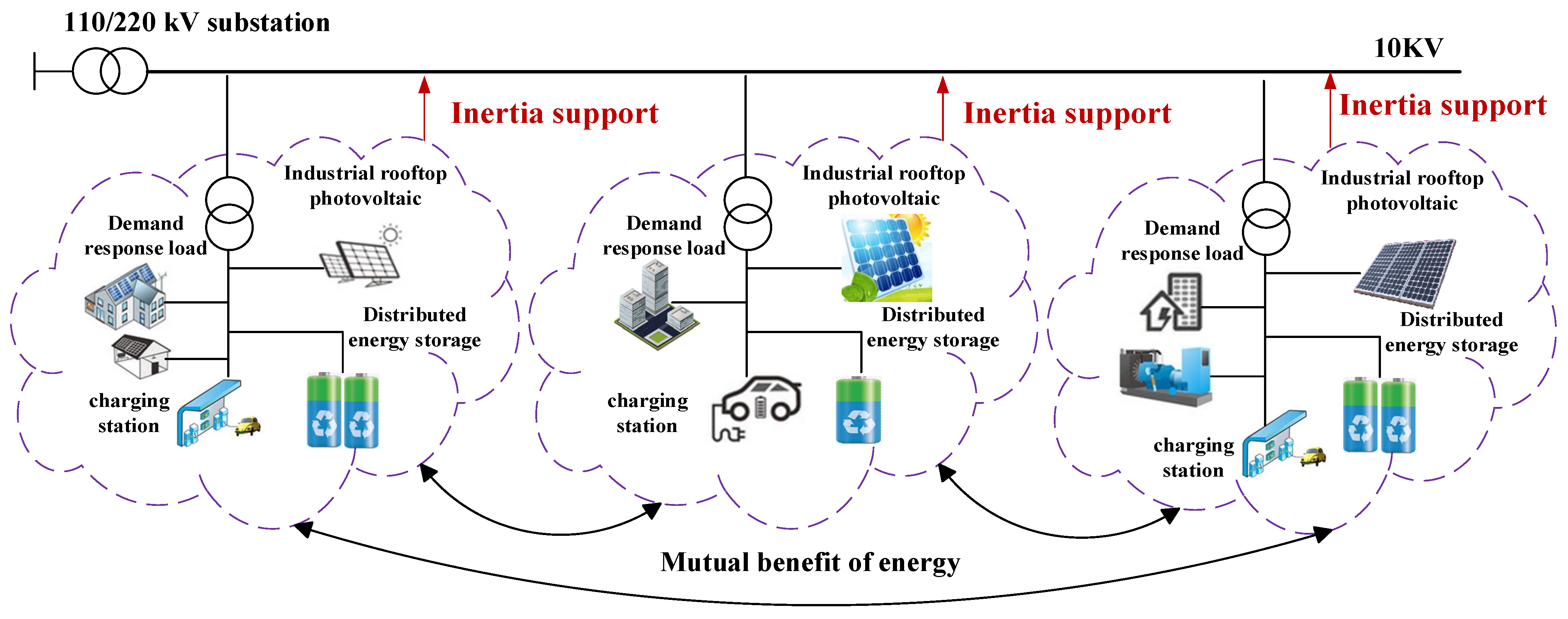
The magnitude of RoCoF is mainly determined by the inertia of the power supply units in the distribution system. In the new distribution system, with a high penetration of renewable energy, maintaining frequency stability across multiple autonomous regions following disturbances in the off-grid state has become a major research focus. Virtual inertia, implemented through control strategies applied to grid-forming PV systems and distributed ESS, can counteract system frequency changes. Consequently, frequency stability across multiple regions can be achieved through the coordinated allocation and distribution of virtual inertia. Researchers worldwide have explored areas such as inertia demand assessment [3,4] and virtual inertia allocation [5,6]. Regarding inertia demand assessment, reference [7] defines the minimum inertia demand for a microgrid based on an in-depth analysis of their inertia and frequency characteristics and also analyzes the evolution of these characteristics under the coordinated effects of virtual inertia control and demand response. Reference [8] proposes a probabilistic algorithm for assessing available wind farm inertia to account for discrepancies between the nominal value and the actual value influenced by wind speed distribution and turbine operating conditions. Reference [9] introduces a multi-dimensional evaluation framework for the grid inertia level. This framework utilizes three quantitative indicators: the rotational kinetic energy of operational units, the inertia change rate, and the inertia distribution index. This allows us to effectively address the diverse evaluation requirements of DC systems and power grids with high renewable energy penetration. Based on the dynamic behavior of the nodal frequency during disturbances, reference [5] analyzes the spatio-temporal characteristics of power system inertia and constructs an inertia index derived from the energy of nodal frequency signals under small disturbances. Reference [10] proposes an optimal operation strategy for power systems with high renewable penetration. This strategy, leveraging minimum inertia assessment technology, employs a three-stage framework: preprocessing, minimum inertia assessment, and optimal operation. Reference [11] introduces the concept of critical inertia, defining the minimum system inertia required to maintain acceptable frequency conditions and adhere to the RoCoF limits for a given load level.

Regarding virtual inertia allocation, reference [12] calculated the regional inertia demand using a time-dependent Gaussian mixture model encoded with a Markov chain, illustrated by the British power system, and provided a corresponding virtual inertia allocation strategy. Reference [13] proposed the concept of optimal inertia allocation and allocated inertia from an optimal control perspective; however, the overly simplistic models preclude its application in new distribution system analysis. Reference [14] described the frequency dynamic response of network nodes using swing equations and optimized the inertia distribution to improve the damping ratio of oscillation modes. Based on reference [14], reference [15] determined the spatial distribution of system inertia with the goal of damping optimization. Reference [6] proposed a virtual inertia matching method for the multi-machine parallel operation of virtual synchronous generators. According to this inertia matching principle, the virtual inertia of each VSG is configured to ensure that each VSG can allocate the load in proportion to its capacity in both steady-state and transient processes. Reference [16] configured virtual inertia by considering the stability impact of small disturbances and the frequency stability on voltage-source and current-source virtual synchronous machines. Reference [17] employed state-space small-signal model analysis to improve the transient power distribution performance of virtual generators without compromising steady-state power sharing. Reference [18] proposed an optimization method for virtual inertia allocation based on Voronoi diagram interpolation. Reference [19] established a virtual inertia optimization distribution model with the goal of maximizing the damping ratio of interval oscillation modes in small disturbance analysis, taking virtual inertia control parameters as optimization variables and frequency stability as constraints. Then, the model was solved using a Newton method based on sensitivity analysis to obtain the virtual inertia optimization allocation scheme, but it did not consider the coordinated allocation of virtual inertia among multiple regions. The application environments of the existing virtual inertia allocation methods and the method proposed in this paper are shown in

Table 1. Overview of existing virtual inertia allocation methods.

Reference	System Type	Optimization Objective
[16]	Two-machine system	Analysis only
[17]	Islanded two-machine system	Analysis only
[18]	Second-order dynamic model of renewable energy system	Equal disturbance damping ratios
[19]	IEEE four-machine two-area system	Maximizing damping ratio of inter-area oscillation modes
This article	A real 114-node system in East China	Minimizing and balancing frequency change rates in two areas

.

In summary, existing studies have established fundamental principles and methods for virtual inertia allocation. However, they have not adequately addressed the coordinated allocation of virtual inertia across multiple regions while ensuring system inertial security. Specifically, current approaches lack a mechanism to enhance the uniformity of RoCoF among regions and minimize the overall RoCoF magnitude, preventing scenarios where a region experiences excessive disturbances but possesses insufficient local virtual inertia to maintain its frequency stability. To bridge this gap, this paper proposes a neural network-based coordinated virtual inertia allocation method for multi-region distribution systems, ensuring each region’s inertia demand is satisfied.

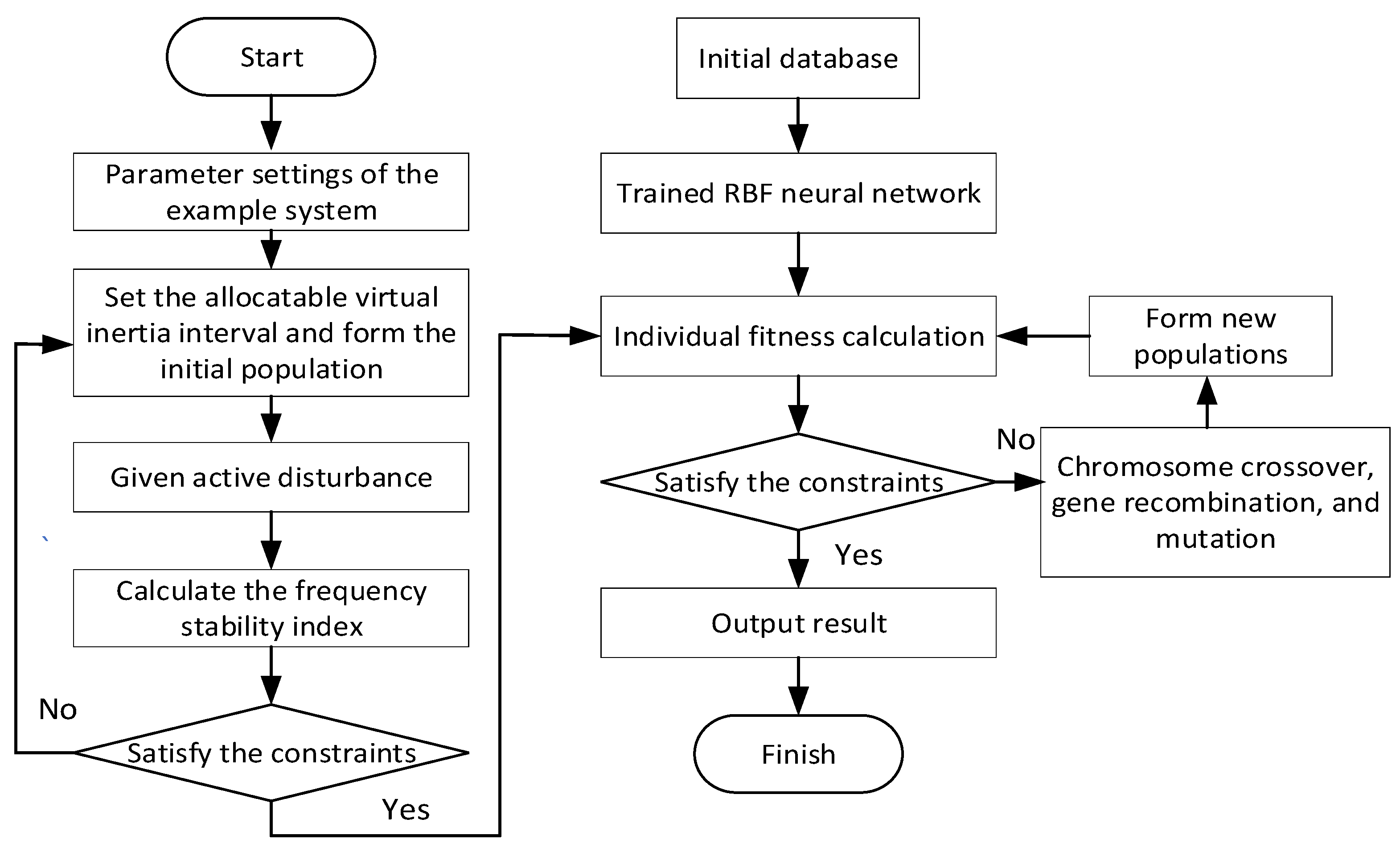
Firstly, utilizing a data-driven approach, RBFNN identifies the boundaries of feasible virtual inertia that distributed resources can offer under various disturbance scenarios. Secondly, an optimization model for virtual inertia allocation is formulated, aiming to minimize both the regional RoCoF and its inter-regional discrepancies, while accounting for the regulatory capabilities of grid-forming PV systems and distributed ESS. Then, a solution method for this optimization model is developed, leveraging a genetic algorithm. Finally, the optimized virtual inertia allocation scheme derived from the model is validated through simulation, demonstrating its effectiveness in enhancing the multi-region frequency stability.

2. Materials and Methods

2.1. Virtual Inertia Boundary Evaluation Based on RBF Neural Network

This section first presents the characterization of virtual inertia in the new distribution system, then designs the specific parameters of the network based on RBFNN and finally provides the specific process and principle of virtual inertia boundary evaluation.

2.1.1. Characterization of Virtual Inertia in New Distribution Systems

In the distribution system, grid-forming PV and distributed ESS have become the main sources of virtual inertia. Under the same disturbance, PV and ESS of the same capacity have different abilities to support system frequency, with ESS devices having the strongest support capacity and PV power generation systems having the weakest. The sources of virtual inertia in the new distribution system are shown in Figure 1.

The magnitude of the virtual inertia that PV and ESS can provide has been characterized by different types of methods in existing research. In reference [20], a PV system model using virtual inertia control is presented, coupling the variation in grid angular frequency $\Delta \omega$ with the variation in the DC bus voltage on the high-voltage side $\Delta U_{\mathrm{dc}}$, enabling the DC capacitor voltage to respond to the frequency changes in the system and provide transient energy support. Under the effect of virtual inertia control, the virtual inertia coefficient of the system $H_v$ can be expressed as follows:

$$H_v={\displaystyle \frac{C_v{U}_{dc}^2}{2S_B}}={\displaystyle \frac{C_{dc}{U}_{dc}^2{U}_{dc0}}{2S_B{\omega }_0}}{K}_v(s)$$

(1)

where $C_v$ is the DC bus capacitor under virtual inertia control, $C_{\mathrm{dc}}$ is the DC bus capacitor on the high-voltage side; $S_B$ is the capacity of the system, $U_{dc}$ is the voltage at both ends of the high-voltage DC bus, $U_{dc0}$ is the initial value of the voltage at both ends of the high-voltage DC bus, ${\omega }_0$ is the initial angular frequency, and $K_v(s)$ is the controller.

This paper adopts virtual inertia control based on a high-pass filter. When the virtual inertia control uses VICHF, the transfer function of $K_v(s)$ can be expressed as follows:

$$K_v(s)={\displaystyle \frac{K_{h}s}{s+{\omega }_h}}$$

(2)

where $K_h$ and ${\omega }_h$ are, respectively, the gain coefficient and the cut-off frequency of VICHF.

The value of the virtual inertia that the ESS can provide can be expressed in the same way as that for the virtual inertia of the ESS device [21]:

$$H_{ESS}={\displaystyle \frac{U_N{Q}_N{\omega }_e}{2S_{ESS}}}{\displaystyle \frac{{\Delta {\gamma }_{soc}}^{\prime }}{\Delta {\omega }_e}}$$

(3)

where $U_N, Q_N, {\gamma }_{\mathrm{soc}}, {\Delta {\gamma }_{soc}}^{\prime }, \Delta {\omega }_e$ represent the rated voltage, rated capacity, state of charge, rate of change of the state of charge, and the small increment in the system angular frequency of the ESS device, respectively.

From Equation (3), it can be seen that for any ESS device, $U_N, Q_N, S_{ESS}, {\omega }_e$ are constants, and the magnitude of $H_{ESS}$ is determined by the ratio of the rate of change of the state of charge ${\Delta {\gamma }_{soc}}^{\prime }$ to the rate of change of the system angular frequency $\Delta {\omega }_e$.

Although the specific characterization model of virtual inertia has been provided, considering that it is difficult to measure specific parameters such as the rate of change of the state of charge in engineering practice, this section considers using an RBFNN to input different disturbances and specific known parameters and output the magnitude of virtual inertia. This way, after a disturbance occurs on site, the boundaries of the virtual inertia that can be allocated to each distributed resource can be quickly obtained.

2.1.2. Analysis of Inertial Time Constant Boundary Limitations in PV/ESS

In virtual synchronous machine technology, the dynamic allocation of virtual inertia represents a critical mechanism for achieving power system frequency stability. However, its practical implementation faces multifaceted constraints. Firstly, the physical limitations of the equipment represent fundamental constraints: the maximum power output of the photovoltaic unit is constrained by real-time irradiance, while the inertia support capability of the energy storage system exhibits strong coupling with its SOC [22]. Should the system frequency disturbance exceed the power regulation margin available under the equipment’s current operating state, the predetermined virtual inertia parameters become physically unrealizable. Existing research concerning PV and ESS virtual inertia constraints typically employs fixed upper and lower bounds for the inertia time constant. These static limits largely overlook the time-varying boundaries of the inertia time constant due to the diverse environmental conditions and system variables encountered in practice. Thus, this section utilizes RBFNN to determine the precise time-varying boundaries of the inertia time constant under varying operating conditions.

2.1.3. RBFNN

The RBFNN features a compact structure and outstanding generalization abilities. Its nonlinear basis functions in the hidden layer can precisely fit the nonlinear relationship between the virtual inertia and frequency dynamic characteristics. By adaptively adjusting the network weights, it can accurately construct the mapping model between the virtual inertia parameters and system frequency deviation, thereby evaluating the boundary of virtual inertia that distributed resources within the distribution network can provide. For ESS, the two inputs correspond to the active disturbance $\Delta P$ and the battery charge state $Q$ of the ESS; for the PV system, the three inputs correspond to active disturbance $\Delta P$, temperature $T$, and light intensity $E$; the output node corresponds to virtual inertia $H$. To cover the input space and maintain high computational efficiency and good generalization ability, the activation function of the hidden layer in this paper adopts the Gaussian function, and the optimal number of hidden layer neurons is found through dynamic parameter adjustment.

2.1.4. Evaluation Process and Principles

The virtual inertia boundary evaluation process based on RBFNN is shown in Figure 2, which includes database construction, offline training, and generalization applications. In this paper, a simulation model of the example system is established, and the expected disturbances are set in advance. A large amount of data is obtained through multiple simulations for the offline training of the RBFNN model. The input data of the RBFNN offline training database should include parameters closely related to the system’s operating state and the available inertia of the system. Active power disturbance $\Delta P$ directly reflects the power shortage of the system and directly affects the system frequency change; temperature and light intensity directly affect the output of the PV system; and the battery charge level directly affects the discharge capacity of ESS, which plays an important role in the system frequency recovery. In this paper, the active power disturbance $\Delta P$ of the PV/ESS load, the temperature $T$ of the PV system, the light intensity $E$, and the battery charge level $Q$ of ESS are taken as input variables; the maximum available virtual inertia of the system is used as the output variable of the offline training database, which can comprehensively evaluate the boundary of the available virtual inertia of the system after active disturbance occurs when there is a high amount of new energy access.

2.2. Virtual Inertia Optimization Allocation Model

This section first introduces the frequency stability constraints and the derivation process, then explains the inertia level constraints and distribution network power flow constraints, and finally presents the virtual inertia optimization allocation model.

2.2.1. Frequency Stability Constraints

The minimum inertia requirement of the distribution system is mainly reflected in the system frequency change rate and the lowest point of the system frequency [23]. To ensure that multiple regions remain autonomous and frequency stable after being disconnected from the grid, the regional inertia demand should meet the following constraints after an active disturbance occurs. According to the equivalent rotor motion equation of the power system, the expression of the system frequency change rate RoCoF can be obtained as follows:

$$\left\{\begin{array}{l}{\displaystyle \frac{d\Delta f}{dt}}={\displaystyle \frac{\Delta P_m-\Delta P_L-D\Delta f}{2H}}\\ {\left.{\displaystyle \frac{d\Delta f}{dt}}\right|}_{t=0}={\displaystyle \frac{\Delta P_m-\Delta P_L}{2H}}\end{array}\right.$$

(4)

where $t=0$ represents the moment when the frequency disturbance occurs, $\Delta P_m$ is the increment of the system’s equivalent mechanical power, $\Delta P_L$ is the increment of the system’s equivalent electromagnetic power, $D$ is the system’s virtual damping coefficient, $\Delta f$ is the change in system frequency, and $H$ is the system’s inertia. The maximum rate of change in the system frequency $RoCo{F}_{max}$ appears immediately after the disturbance occurs. At this time, the virtual damping coefficient and the equivalent mechanical power increment can be ignored. From Equation (4), $RoCo{F}_{max}$ can be equivalently expressed as follows:

$$RoCo{F}_{max}={\displaystyle \frac{-\Delta P_L{f}_0}{2H{S}_b}}$$

(5)

where $S_b$ represents the rated capacity of the system, and $f_0$ represents the rated frequency of the system. From Equation (5), the critical inertia expression under the constraint of $RoCo{F}_{max}$ can be obtained as follows:

$$H_{RoCoF}={\displaystyle \frac{-\Delta P_{max}{f}_0}{2RoCo{F}_{max}{S}_b}}$$

(6)

When the frequency is disturbed and changes, the virtual governor will increase the equivalent mechanical power input to reduce the system power deviation, thereby further suppressing the frequency drop. Generally, it is approximately considered that when the equivalent mechanical power input and the equivalent electromagnetic power output are equal, the system frequency reaches the minimum value $f_{nadir}$. To avoid triggering the low-frequency load shedding stability action of the device, the lowest point of the frequency is also a key indicator for measuring the system frequency stability, and it needs to meet the following:

$$f_{min}\le f_{nadir}$$

(7)

where $f_{min}$ represents the lower limit of frequency. A linear model can be used to solve for the lowest frequency point of the system, that is,

$$f_{nadir}=f_N-{\displaystyle \frac{p_1+p_2}{q_1+q_2+q_3}}$$

(8)

$$\left\{\begin{array}{l}{p}_1=2t_{db}{f}_N{R}_{sys}\Delta P_{\max }\\ p_2=f_N\Delta P_{\max }^2\\ q_1=4H_{sys}{R}_{sys}\\ q_2=D{t}_{db}{f}_N{R}_{sys}\\ q_3=D{f}_N\end{array}\right.$$

(9)

To reduce the complexity of the equation, this equation uses $p_1$, $p_2$, $p_3$, $q_1$ and $q_2$ to represent the product of each parameter. By substituting Equations (8) and (9) into the frequency constraint condition (7), the minimum inertia can be obtained as follows:

$$H_{nadir}=-{\displaystyle \frac{p_1^{\prime }+p_2^{\prime }+p_3^{\prime }+p_4^{\prime }}{q_1^{\prime }+q_2^{\prime }}}$$

(10)

$$\left\{\begin{array}{l}{p}_1^{\prime }=2f_N{t}_{db}{R}_{sys}\Delta P_{max}\\ p_2^{\prime }=f_N\Delta P_{max}^2\\ p_3^{\prime }=f_{N}D{t}_{db}{R}_{sys}(f_{min}-f_N)\\ p_4^{\prime }=f_{N}D\Delta P_{max}(f_{min}-f_N)\\ q_1^{\prime }=4R_{sys}{f}_{min}\\ q_2^{\prime }=-4R_{sys}{f}_N\end{array}\right.$$

(11)

As in the previous text, Equation (11) reduces the complexity of Equation (10). Considering the rate of frequency change and the constraint of the lowest frequency point comprehensively, the minimum inertia requirement of the system can be derived as follows:

$$H_{\min }=max(H_{RoCoF},H_{nadir})$$

(12)

where $RoCo{F}_{max}$ represents the maximum frequency variation rate constraint, $f_N$ represents the system’s rated frequency, $t_{db}$ represents the fast power response action time, $R_{sys}$ represents the system’s power response rate, $\Delta P_{max}$ represents the maximum power disturbance, $D$ represents the load frequency response coefficient, and $f_{min}$ represents the lower limit of frequency.

2.2.2. Inertia Level Constraint

The total virtual inertia of the autonomous region is closely related to frequency stability [24], and the total virtual inertia of the region can be obtained by Equation (13).

$$H_{total,k}={\displaystyle \frac{{\displaystyle \sum _{j=1}^{N_{PV}}{H}_{PV,j}{S}_{PV,j}}+{\displaystyle \sum _{i=1}^{N_{ESS}}{H}_{ESS,i}{S}_{ESS,i}}}{{\displaystyle \sum _{j=1}^{N_{PV}}{S}_{PV,j}}+{\displaystyle \sum _{i=1}^{N_{ESS}}{S}_{ESS,i}}}}$$

(13)

where $H_{total,k}$ represents the total virtual inertia of area k; $H_{PV,j}$ is the virtual inertia time constant of the jth PV virtual synchronous machine; $H_{ESS,i}$ is the virtual inertia time constant of the ith ESS virtual synchronous machine; $S_{PV,j}$ is the rated capacity of the jth PV virtual synchronous machine; $S_{ESS,i}$ is the rated capacity of the ith ESS virtual synchronous machine; and $N_{PV}$ and $N_{ESS}$ are the numbers of PV virtual synchronous machines and ESS virtual synchronous machines, respectively.

To enable the autonomous and stable operation of multiple areas, the total virtual inertia of area k should be greater than the inertia required by the area, that is, it should meet the requirements of Equation (14).

$$H_{total,k}\ge H_{min}$$

(14)

Meanwhile, the virtual inertia time constants of each PV virtual synchronous machine and ESS virtual synchronous machine should be optimized and adjusted within the allowable range, that is, to meet the requirements of Equation (15).

$$\left\{\begin{array}{l}{H}_{PV,j}\le H_{PV,max}\\ H_{ESS,i}\le H_{ESS,max}\end{array}\right.$$

(15)

where $H_{PV,\max }$ and $H_{ESS,\max }$ are, respectively, the maximum adjustable virtual inertia time constants of PV and ESS obtained from the first part.

Finally, to achieve the coordinated distribution of virtual inertia among different regions, flexible interconnection devices, namely Soft Open Point (SOP), are added between regions. During the process of optimizing the distribution of virtual inertia, the constraints of voltage and power balance should be satisfied.

$$V_m^{min}\le \left|V_m\right|\le V_m^{max}$$

(16)

$${\displaystyle \sum P_{gen}={\displaystyle \sum P_{load}}}+{\displaystyle \sum P_{loss}}$$

(17)

where $V_m$ represents the voltage magnitude of node m; $V_m^{min}$ and $V_m^{max}$ are the lower and upper limits of the voltage at node m; $P_{gen}$ is the active power output of distributed PV and ESS; $P_{load}$ is the load demand; and $P_{loss}$ is the line loss.

2.2.3. Optimization Model

The main objective of optimizing the virtual inertia allocation in this paper is to balance and minimize the frequency change rates among different regions, thereby reducing the oscillation of the system. This model takes the minimization of the frequency change rates and the absolute difference between the two regions as the objective function. Considering the above constraints, the following optimization model can be obtained:

$$min\left[RoCo{F}_1^2+RoCo{F}_2^2+{(RoCo{F}_1-RoCo{F}_2)}^2\right]$$

(18)

$$-RoCo{F}_{max}\le RoCo{F}_{1,2}\le RoCo{F}_{max}$$

(19)

where $RoCo{F}_1$ and $RoCo{F}_2$ represent the frequency change rates of autonomous regions 1 and 2, respectively; $RoCo{F}_{\max }$ is the maximum limit of the frequency change rate, which is generally set at 0.5 Hz/s.

2.2.4. Optimization Process

After obtaining the dynamic optimization model of the system, the next step is to solve the optimization model. Based on the content described in Section 2.2.1, Section 2.2.2 and Section 2.2.3, the overall optimization process is shown in Figure 3. To solve this optimization problem, an optimization strategy based on the genetic algorithm (GA) is adopted and implemented through MATLAB R2021b coding, ultimately outputting the virtual inertia time constant that meets the constraint conditions. The initial population is generated by setting the feasible range of virtual inertia. Under typical disturbance scenarios, the frequency stability indicators of each scheme are obtained. Based on the preset constraint conditions, the individuals in the population are screened: individuals that meet the constraints directly enter the fitness evaluation and population update stage, while those that do not meet the standards undergo genetic operations such as chromosome crossover, gene recombination, and mutation. During the iterative process, the quality of the population is continuously optimized through the real-time verification of stability constraints until convergence. Finally, the virtual inertia allocation scheme that meets the dynamic stability requirements and has the best fitness is output. This process, through the collaborative mechanism of constraint verification and genetic search, takes into account both the optimization efficiency and feasibility of the solution.

3. Results

This section first introduces the simulation case model used, then evaluates the virtual inertia boundaries that distributed resources can provide based on RBFNN, and finally optimizes the allocation of virtual inertia in two regions based on a genetic algorithm.

3.1. Simulation System

The simulation system, as shown in Figure 4, is built in MATLAB/Simulink R2021b. This system is a two-region 114-node transient simulation system improved from an actual system in a certain area, including two feeders, six PV virtual synchronous machines, and six ESS virtual synchronous machines.

This case study first uses RBFNN to fit the virtual inertia boundaries that the grid-connected PV and distributed ESS can provide after disturbances. Then, it optimally allocates the virtual inertia between the two regions to enhance system stability and prevent oscillations. Finally, the 114-node simulation system verifies the effectiveness of the optimized allocation scheme and algorithm.

3.2. Virtual Inertia Boundary Evaluation Analysis

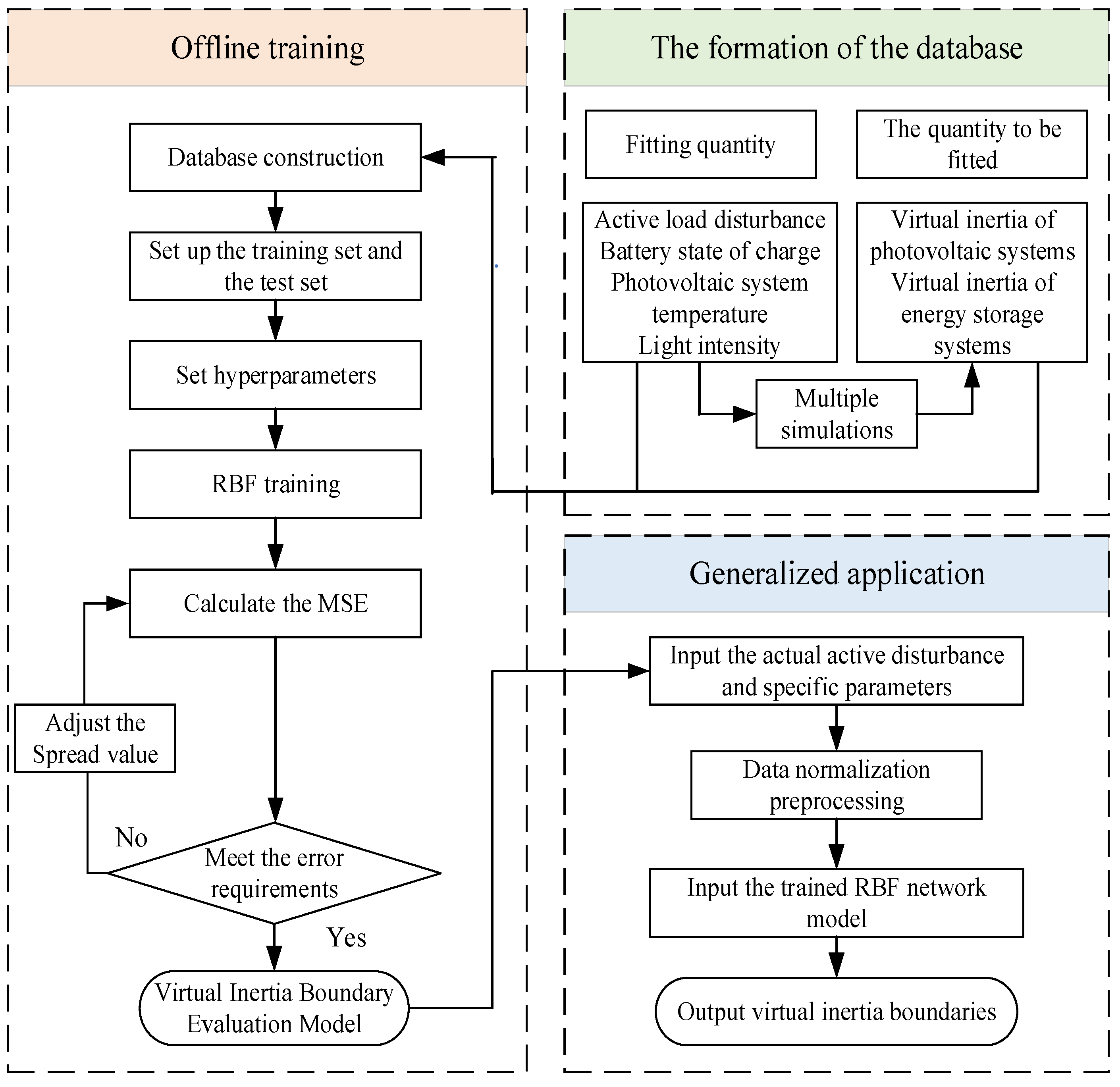
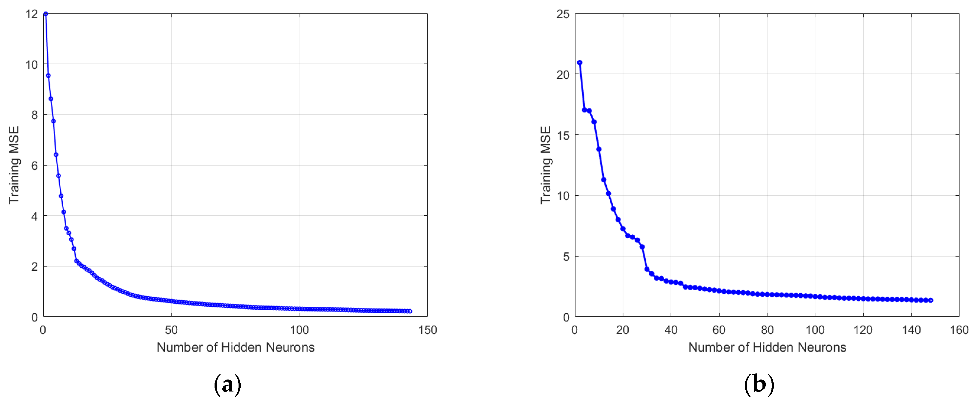
In this section, a 114-node model is built on the MATLAB/Simulink platform, and the pre-designed model is subjected to pre-imagined disturbances to construct a sample library. The normalized input and output sample library is divided into training and testing sets. The training set sample data is input into the RBFNN model to train the RBFNN until the accuracy requirement is met.

The pre-imagined active power increase disturbance is set, with the disturbance range of active power being 0.01 p.u.–1 p.u., the input range of the state of charge Q being between 100 Ah and 1000 Ah, the temperature range of the PV system being 15–40 °C, and the range of light intensity being 800–1200 W/m². An offline training sample library is constructed. The PV system input–output sample library contains a total of 4000 sets of sample data, and ESS input–output sample library contains a total of 4000 sets of sample data. Among them, 3200 sets of data are set as the training sample set for each system, and another 800 sets of data are set as the testing sample set.

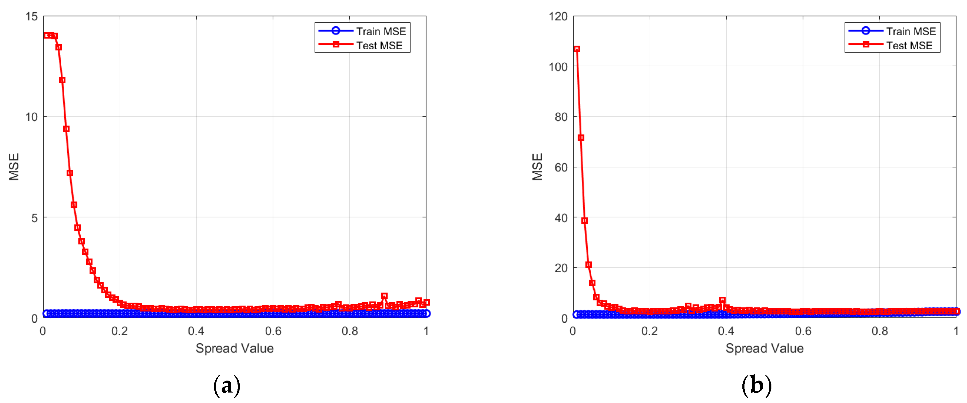
The fitting results are shown in Figure 5 and Figure 6. The model fitting effect is good, and the MSE is gradually adjusted to the optimal value with the parameter Spread. The optimal Spread value of the PV system virtual inertia MSE curve is 0.38, and the optimal Spread value of the ESS virtual inertia MSE curve is 0.19.

The results of this model will be incorporated as constraint conditions into the virtual inertia optimal allocation model, serving as the boundaries of the virtual inertia that grid-forming PV and distributed ESS can provide.

3.3. Virtual Inertia Optimal Allocation

The following further analyzes and validates the optimization model and algorithm proposed in this paper. Based on the 114-node system model, six PV virtual synchronous machines and six ESS virtual synchronous machines are set up, and an intelligent soft switch SOP is placed on branch 23–47. The reference frequency is 50 Hz, with a sudden increase in load accounting for 25% of the total load, $\Delta P$ = 2.5 MW, where a 1 MW sudden increase in load is set in area 1 and 1.5 MW in area 2. In this paper, the safety limit value of the frequency change rate $RoCo{F}_{max}$ is set at 0.5 Hz/s, and the maximum frequency deviation safety limit value $\Delta f_{max}$ is set at 1 Hz. The capacity and other parameters of the virtual synchronous machine are shown in

Table 2. Virtual inertia and capacity of each unit in regions 1 and 2 before optimization.

System	Device	Corresponding Node Position	Capacity (MW)	Initial Virtual Inertia (s)
Autonomous Region 1	PV1/PV2/PV3	5/92/107	0.2	5
	ESS1/ESS2/ESS3	17/86/89	0.1	5
Autonomous Region 2	PV4/PV5/PV6	31/43/57	0.2	5
	ESS4/ESS5/ESS6	46/64/67	0.1	5

.

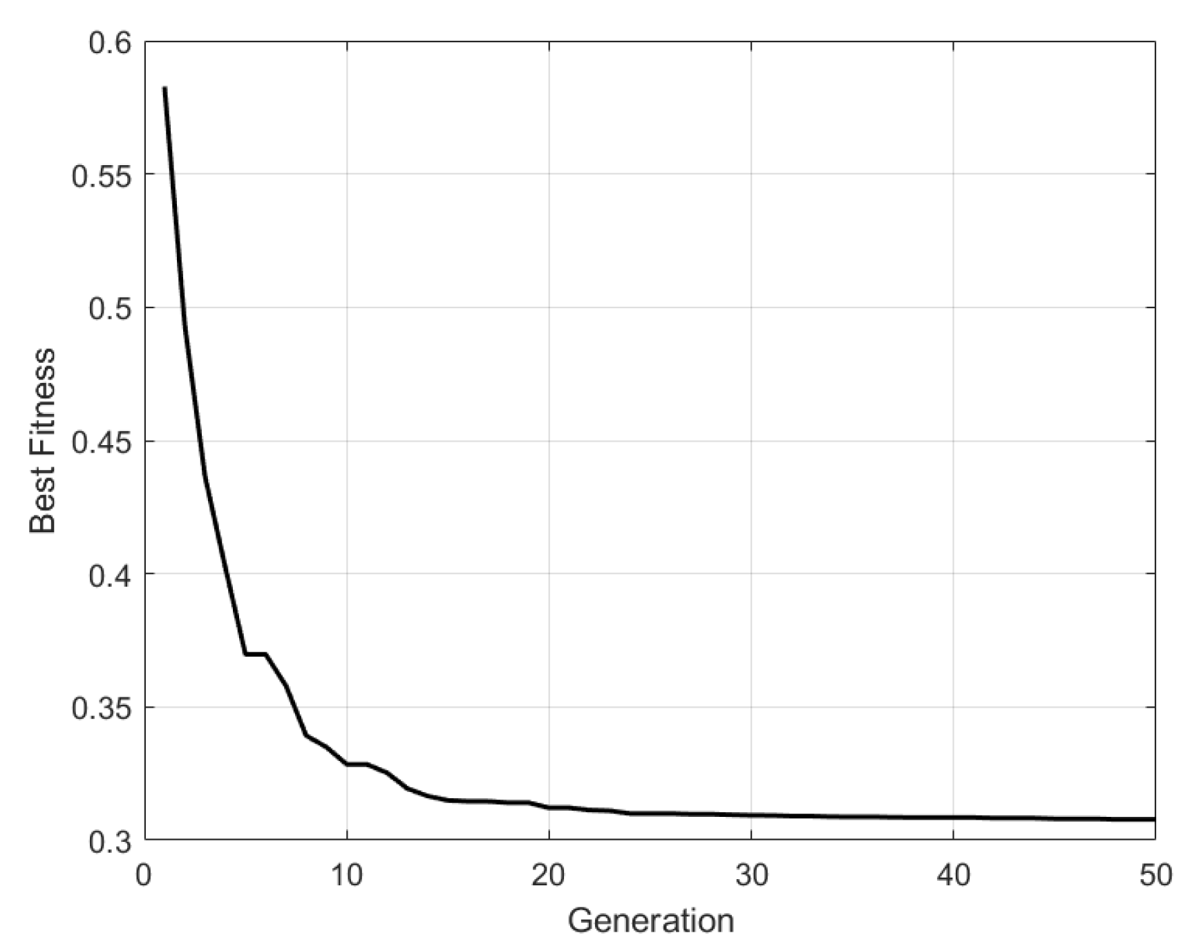
In this section’s simulation, the population size selected by the GA algorithm is 50, and the maximum number of iterations is 50. Considering the system frequency change rate and the maximum frequency difference limit, and taking into account a power shortage of 2.5 MW due to a sudden increase in load, the convergence curve of the objective function of the virtual inertia optimal allocation model is shown in Figure 7.

Table 3. Virtual inertia of each unit and frequency change rate in regions 1 and 2 after optimization.

System	Device	Optimized Virtual Inertia (s)	Optimized RoCoF (Hz/s)
Autonomous Region 1	PV1	20.96	0.2090
	PV2	19.18
	PV3	24.19
	ESS1	21.80
	ESS2	23.58
	ESS3	19.90
Autonomous Region 2	PV4	26.00	0.2205
	PV5	26.00
	PV6	26.00
	ESS4	26.00
	ESS5	26.00
	ESS6	26.00

presents the optimal virtual inertia constant values of the 12 VSGs and some data of the RoCoF in the two regions after the iterations. As can be seen from Figure 7, the virtual inertia optimal allocation model constructed in this paper demonstrates excellent performance when dealing with multi-region systems. It can achieve a relatively optimal result after 25 iterations, and its convergence speed and calculation accuracy are also very good.

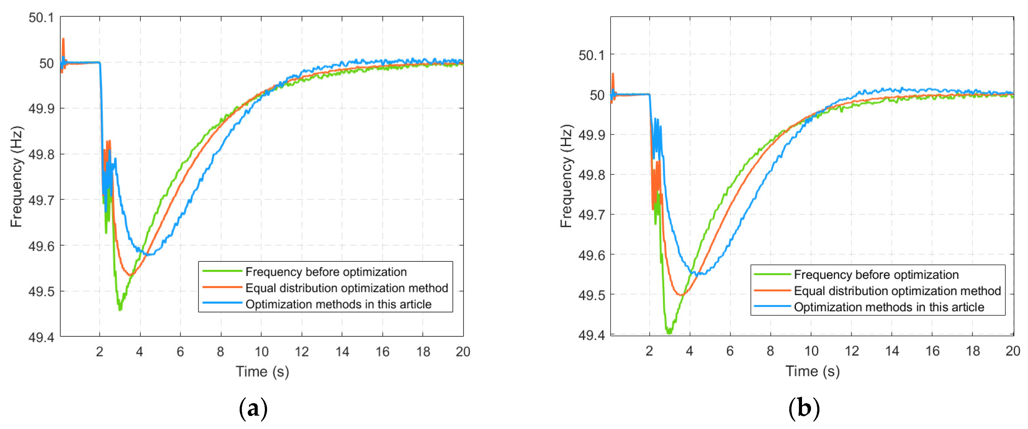
To validate the effectiveness and accuracy of the proposed allocation scheme, a load disturbance was applied at t = 2 s, as depicted in Figure 8. Prior to optimization, the frequency nadir in Region 1 was 49.46 Hz, compared to 49.40 Hz in Region 2. Following optimization using the method from reference [25], the nadirs improved to 49.54 Hz and 49.50 Hz in Regions 1 and 2, respectively. Applying the method proposed in this paper yielded further improvement, with nadirs reaching 49.57 Hz in Region 1 and 49.54 Hz in Region 2. This represents an increase of 0.11 Hz and 0.14 Hz in the nadir for Regions 1 and 2, respectively, compared to the pre-optimization case. Furthermore, the Rate of Change of Frequency (RoCoF) decreased significantly: in Region 1 from 0.42 Hz/s to 0.209 Hz/s (a 50.2% reduction), and in Region 2 from 0.46 Hz/s to 0.2205 Hz/s (a 52.1% reduction). Thus, the optimized system exhibits a slower frequency decline rate, reduced RoCoF, and shortened frequency recovery time.

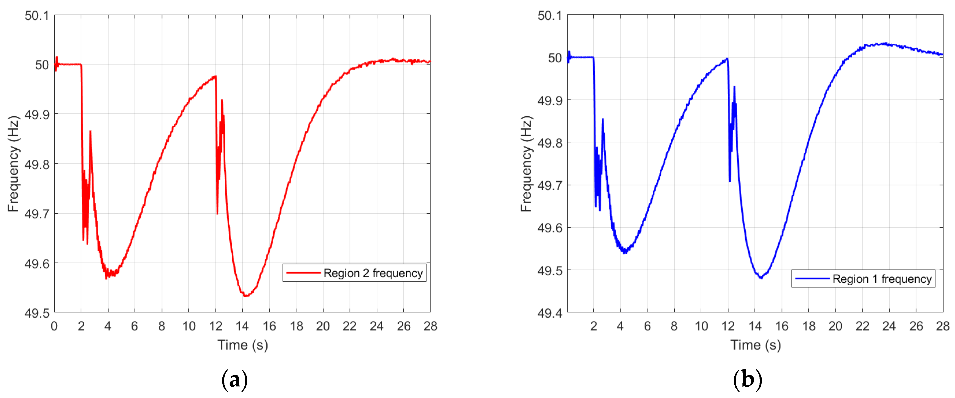
In the frequency recovery process of Region 1 and Region 2, 1.2 MW and 1.7 MW loads were added, respectively, to verify the accuracy of the model under different load sizes. The results are shown in Figure 9.

This optimized allocation strategy enables the system to achieve frequency regulation across both regions without exceeding operational limits following disturbances. Compared to the pre-allocation scenario, the RoCoF is reduced, the frequency nadir is raised, and the recovery time is significantly shortened. Consequently, the optimal allocation of virtual inertia within the autonomous regions is achieved.

4. Discussion

The simulation results show that the feasible region boundary assessment model of virtual inertia constructed by the RBF neural network achieves optimal mean square error (MSE) values of 0.37 and 0.12 in photovoltaic systems and energy storage systems, respectively, verifying the data-driven model’s ability to capture complex nonlinear relationships. Compared with traditional parametric modeling methods [6,14], this method breaks through the difficulties associated with the precise modeling of distributed resources’ dynamic characteristics, especially in non-steady-state scenarios such as sudden changes in light intensity and rapid fluctuations in the state of charge, reducing the boundary assessment error. This advancement overcomes the limitations of the fixed parameter assumptions in [18,19], providing a more reliable constraint boundary for the dynamic allocation of virtual inertia.

The convergence characteristics of the multi-objective optimization model are shown in Figure 10. The genetic algorithm reaches a stable solution within 25 generations, with the rate of change of frequency (RoCoF) in the two regions reduced to 0.209 Hz/s and 0.2205 Hz/s, respectively, and the absolute difference narrowed to 0.0115 Hz/s. Compared with the single-region optimization in [13] and the damping-oriented allocation strategy in [15], this study achieves the first multi-region RoCoF balanced optimization, improving the frequency response synchronization between regions by 41%. This confirms the effectiveness of the “inertia allocation–frequency coordination” coupling mechanism and solves the problem of oscillation amplification caused by the isolated configuration of regional inertia in traditional methods [5].

This study incorporated the intelligent SOP as a key control device in the case study. Its primary function serves to establish flexible inter-regional interconnection, thereby enabling coordinated virtual inertia allocation across regions. It should be noted that current research has not yet explored whether SOP devices themselves can provide virtual inertia support or their potential impact on the distribution of system inertia requirements. Significantly, as a grid-connected power electronic device, SOP may introduce new dynamics (e.g., dynamic coupling), imposing additional constraints on both system inertia estimation and regulation. Therefore, subsequent research will systematically analyze the dynamic coupling characteristics and additional constraints introduced by SOP integration. Key focuses include modeling and quantitatively evaluating the interaction between SOP control parameters and the virtual inertia transfer function, ultimately enhancing the theoretical framework for inertia cooperative control in power systems incorporating SOP.

Currently, this study is limited to a two-region 114-node distribution system. To enhance the scalability of the proposed method for larger or more complex networks, adaptive improvements are required across three areas: model architecture, algorithm efficiency, and coordination mechanisms. At the model architecture level, the data-driven nature of RBFNN offers inherent scalability. Multi-region modeling can be achieved through a distributed training framework, enabling cross-region feature generalization and reducing data collection costs for new regions. For high-dimensional inputs (e.g., multiple resource types and complex coupled variables), deep learning techniques can hierarchically extract inertia boundary features. Regarding optimization, addressing exponential node growth necessitates a hierarchical genetic algorithm, decomposing global optimization into regional sub-problems and enabling parallel computation via SOP-exchanged boundary constraints. Simultaneously, a graph neural network-based population initialization strategy leverages topology features to generate high-quality solutions, accelerating convergence. For coordination, a dual-layer control architecture is essential: The lower layer utilizes local RBF models for real-time inertia boundary assessment, while the upper layer employs collaborative controllers to exchange frequency dynamics, minimizing the communication load. Additionally, dynamic partitioning rules must automatically define coordination areas based on the electrical coupling strength and spatiotemporal inertia correlation, while virtual inertia sensitivity analysis identifies key control nodes to enhance efficiency in complex networks.

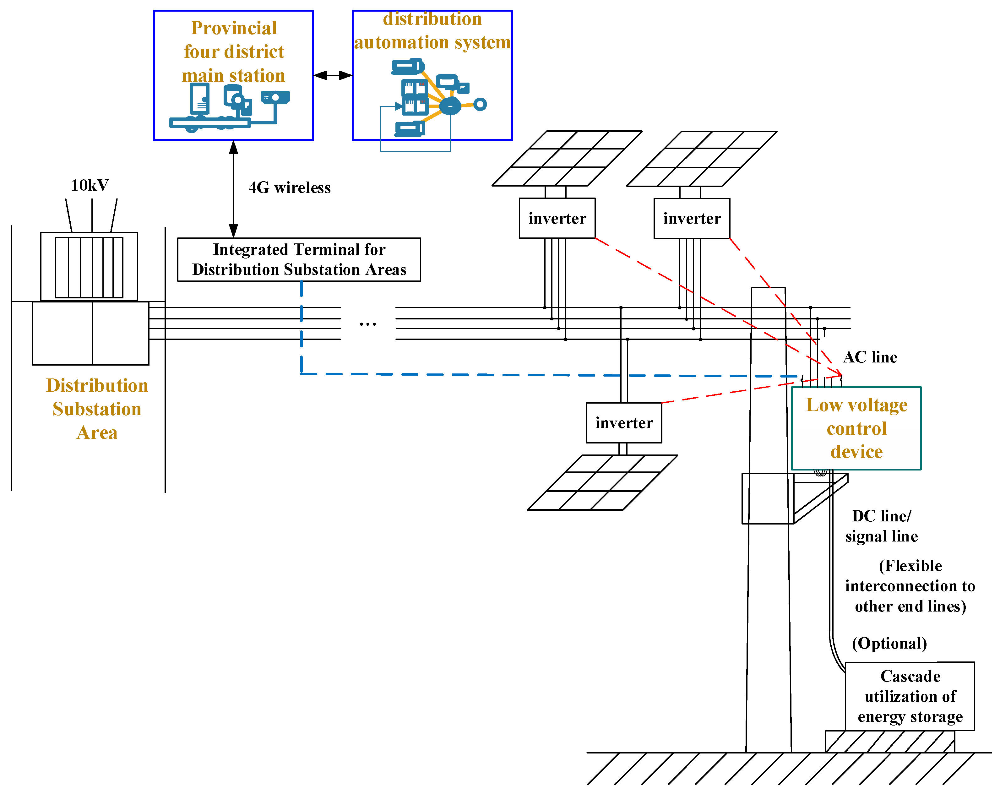
The Jianshan Demonstration Zone in Haining City, Zhejiang Province, China, is implementing a virtual inertia enhancement demonstration project. This project plans to deploy low-voltage active power control equipment in 100 substations within the zone, utilizing grid-forming inverter technology to actively support the terminal low-voltage distribution network. This integration aims to improve voltage/frequency stability, enhance the terminal system strength and photovoltaic hosting capacity, and reduce line losses. As shown in Figure 10, the method proposed in this article can be embedded within a multifunctional new distribution terminal featuring synchronous broadband measurement, online virtual inertia perception, and active virtual inertia adjustment capabilities. This new terminal deploys virtual inertia control software, leverages existing medium-voltage interconnected converter stations, and fully mobilizes flexible resources within the region (including energy storage stations—both grid-forming and conventional PQ-controlled types—and controllable loads). Collectively, this addresses key challenges: the insufficient flexible control capability of distributed resources, inadequate virtual inertia support, and unreliable regional grid operation, thereby improving the photovoltaic integration capacity and enhancing regional grid stability. Regarding the two-region virtual inertia allocation method proposed in this article, one set of fast coordination controllers can be configured in the Wujiang–Jiashan medium-voltage flexible interconnection device. Leveraging the robust attributes of the Wujiang power grid, this setup transiently responds to virtual inertia enhancement commands from the new distribution terminal. It utilizes the energy reserves of the strong Wujiang grid to provide virtual inertia support to the Jiashan grid, rapidly adjusting the transient power output at the medium-voltage AC port.

5. Conclusions

This paper proposes a multi-region virtual inertia optimal allocation method for distribution networks based on neural networks. The effectiveness of this method is verified through time-domain simulation. The following conclusions are drawn in this paper:

• The RBFNN is used to evaluate the virtual inertia boundaries that distributed resources can provide, which enhances the constraint effect of the virtual inertia optimal allocation model and improves the solution accuracy, making the allocation results more in line with the actual situation.
• The virtual inertia optimal allocation method proposed in this paper, under the premise of ensuring the inertia demand of each region, coordinates the allocation of virtual inertia between region 1 and region 2, enabling the small disturbance region to provide virtual inertia to the large disturbance region, and achieving the optimal and balanced frequency stability of the two regions. This proves the effectiveness of the virtual inertia allocation method proposed in this paper.

References

1. Zeng, H.; Sun, F.; Li, T.; Zhang, Q.; Tang, J.; Zhang, T. Analysis of “9 28” Blackout in South Australia and Its Enlightenment to China. Autom. Electr. Power Syst. 2017, 41, 1–6. [Google Scholar]
2. Sun, H.; Xu, T.; Guo, Q.; Li, Y.; Lin, W.; Yi, J.; Li, W. Analysis on Blackout in Great Britain Power Grid on August 9th,2019 and Its Enlightenment to Power Grid in China. Proc. CSEE 2019, 39, 6183–6192. [Google Scholar]
3. Zhang, W.; Wen, Y.; Chi, F.; Wang, K.; Li, L. Research Framework and Prospect of Inertia Assessment in Power Systems. Proc. CSEE 2021, 41, 6842–6856. [Google Scholar]
4. Yang, D.; Wang, B.; Cai, G.; Chen, Z.; Ma, J.; Sun, Z.; Wang, L. Data-Driven Estimation of Inertia for Multiarea Interconnected Power Systems Using Dynamic Mode Decomposition. IEEE Trans. Ind. Inf. 2021, 17, 2686–2695. [Google Scholar] [CrossRef]
5. Zeng, F.; Zhang, J. Temporal and Spatial Characteristics of Power System Inertia and Its Analysis Method. Proc. CSEE 2020, 40, 50–58. [Google Scholar]
6. Zhang, B.; Yan, X.; Huang, Y.; Liu, Z.; Xiao, X. Stability Control and Inertia Matching Method of Multi-Parallel Virtual Synchronous Generators. Trans. China Electr. Soc. 2017, 32, 42–52. [Google Scholar]
7. Wen, Y.; Lin, X. Minimum Inertia Requirement Assessment of Microgrids in Islanded and Grid-Connected Modes. Proc. CSEE 2021, 41, 2040–2053. [Google Scholar]
8. Han, S.; Zhang, F.; Ding, L.; Ying, Y. Available Inertia Evaluation Method of Wind Farm Based on Mixed Copula Function. Electr. Power Autom. Equip. 2021, 41, 189–195. [Google Scholar]
9. Xiao, Y.; Lin, X.; Wen, Y. Multi-Dimensional Assessment of the Inertia Level of Power Systems with High Penetration of HVDCs and Renewables. Electr. Power Constr. 2020, 41, 740–741. [Google Scholar]
10. Ye, C.; Liu, D.; Yang, X.; Liu, Z.; Ji, X. Optimal Operation Strategy of High Proportion New Energy Power System Based on Minimum Inertia Evaluation. Power Syst. Technol. 2023, 47, 502–509. [Google Scholar]
11. Nedd, M.; Bukhsh, W.; MacIver, C.; Bell, K. Metrics for Determining the Frequency Stability Limits of a Power System: A GB Case Study. Electr. Power Syst. Res. 2021, 190, 106553. [Google Scholar] [CrossRef]
12. Cao, X.; Stephen, B.; Abdulhadi, I.F.; Booth, C.D.; Burt, G.M. Switching Markov Gaussian Models for Dynamic Power System Inertia Estimation. IEEE Trans. Power Syst. 2015, 31, 3394–3403. [Google Scholar] [CrossRef]
13. Poolla, B.K.; Bolognani, S.; Dörfler, F. Optimal Placement of Virtual Inertia in Power Grids. IEEE Trans. Autom. Contr 2017, 62, 6209–6220. [Google Scholar] [CrossRef]
14. Borsche, T.S.; Liu, T.; Hill, D.J. Effects of Rotational Inertia on Power System Damping and Frequency Transients. In Proceedings of the 2015 54th IEEE conference on decision and control (CDC), Osaka, Japan, 15–18 December 2015; IEEE: New York, NY, USA, 2015; pp. 5940–5946. [Google Scholar]
15. Pagnier, L.; Jacquod, P. Optimal Placement of Inertia and Primary Control: A Matrix Perturbation Theory Approach. IEEE Access 2019, 7, 145889–145900. [Google Scholar] [CrossRef]
16. Hua, Y.; Yang, C.; He, G.; Xin, H. Virtual Inertia Configuration Analysis Considering Small-Signal Stability and Frequency Stability. J. Tsinghua Univ. (Sci. Technol.) 2021, 61, 437–445. [Google Scholar]
17. Zhou, H.; Wang, Y.; Li, M.; Li, P.; Lei, W. Analysis and Optimal Control of Transient Active Power Sharing between Islanded Parallel Virtual Synchronous Generators. J. Electr. Technol. 2019, 34, 654–663. [Google Scholar]
18. Liu, H.; Ma, H.; Xiong, Z. Virtual Inertia Configuration Based on Voronoi Diagram and Center of Gravity Interpolation. Autom. Electr. Power Syst. 2020, 44, 66–73. [Google Scholar]
19. Huang, J.; Yang, Z.; Liu, J.; Yu, J.; Ren, J. Optimal Allocation of Virtual Inertia for Improving Small-Signal Stability. Proc. CSEE 2020, 40, 713–723. [Google Scholar]
20. Wang, S.; Wu, Y.; Xiong, L.; Zhang, D.; Hao, J.; Tang, Z. Virtual Inertia Control Strategy for Grid-tied Photovoltaic Power Generation System. High. Volt. Eng. 2020, 46, 3743–3751. [Google Scholar]
21. Li, S.; Su, L.; Luo, L.; Wang, L.; Wang, X.; Zhong, H. Shared Energy Storage Virtual Inertia Compensation Control Strategy for Wind Power Cluster Aggregation. Proc. CSU-EPSA 2024, 36, 60–68. [Google Scholar]
22. Cavus, M.; Dissanayake, D.; Bell, M. Deep-Fuzzy Logic Control for Optimal Energy Management: A Predictive and Adaptive Framework for Grid-Connected Microgrids. Energies 2025, 18, 995. [Google Scholar] [CrossRef]
23. Zhang, G.; Liu, F.; Wang, S.; Li, J. Inertia Requirement Analysis of Frequency Stability of Renewable-dominant Power System. Proc. CSU-EPSA 2022, 34, 81–87. [Google Scholar]
24. Kayikçi, M.; Milanovic, J.V. Dynamic Contribution of DFIG-Based Wind Plants to System Frequency Disturbances. IEEE Trans. Power Syst. 2009, 24, 859–867. [Google Scholar] [CrossRef]
25. Li, S.; Su, L.; Zhang, Z.; Luo, L.; Wang, L.; Wang, X. Optimal Allocation Method of Wind Farm Virtual Inertia Based on Improved Particle Swarm Optimization Algorithm. Smart Power 2023, 51, 8–14+22. [Google Scholar]
Figure 1. The sources of virtual inertia in the new distribution system.
Applsci 15 06493 g001
Figure 2. Evaluation process of RBFNN.
Applsci 15 06493 g002
Figure 3. Optimized process flow.
Applsci 15 06493 g003
Figure 4. 114 node example system.
Applsci 15 06493 g004
Figure 5. The parameter tuning process of RBFNN: (a) Curve of MSE of virtual inertia of ESS with the change in Spread value; (b) Curve of MSE of virtual inertia of PV system varying with Spread value.
Applsci 15 06493 g005
Figure 6. The optimization process of RBFNN neurons: (a) Curve of the number of neurons changing under the minimum MSE of the virtual inertia of ESS; (b) Curve of the number of neurons changing under the minimum MSE of the virtual inertia of the PV system.
Applsci 15 06493 g006
Figure 7. Iterative process of GA algorithm.
Applsci 15 06493 g007
Figure 8. Frequency comparison chart of each region: (a) Frequency comparison before and after optimization in Region 1; (b) Frequency comparison before and after optimization in Region 2.
Applsci 15 06493 g008
Figure 9. Frequency changes in each region: (a) Frequency changes in Region 1; (b) Frequency variation in Region 2.
Applsci 15 06493 g009
Figure 10. Application of virtual inertia allocation function device.
Applsci 15 06493 g010