Abstract
The present research analyzed the nonlinear vibration of a CNTRC embedded in a nonlinear Winkler–Pasternak foundation in the presence of an electromagnetic actuator and mechanical impact. A higher-order shear deformation beam theory was applied to various models, as well as Euler–Bernoulli, Timoshenko, Reddy, and other beams, using a unified NSGT. The governing equations were obtained based on the extended shear and normal strain component of the von Karman theory and a Hamilton principle. The system was discretized by means of the Galerkin–Bubnov procedure, and the OAFM was applied to solve a complex nonlinear problem. The buckling and bending problems were studied analytically by using the HPM, the Galerkin method in combination with the weighted residual method, and finally, by the optimization of results for a simply supported composite beam. These results were validated by comparing our results for the linear problem with those available in literature, and a good agreement was proved. The influence of some parameters was examined. The results obtained for the extended models of the Euler–Bernoulli and Timoshenko beams were almost the same for the linear cases, but the results of the nonlinear cases were substantially different in comparison with the results obtained for the linear cases.
1. Introduction
It is known that CNTs are one of the most promising reinforced materials in many engineering applications, such as satellite antennas, nanoelectronics, nanosensors, automotives, aircrafts, turbine blades, robot arms, and so on. Various models of CNT along with non-classical theories have been proposed in the last years to study vibration, buckling, or bending problems. Composites based on nanotubes offer strength-to-weight ratios. NASA and companies such as Samsung or NEC have invested tremendously and demonstrated product quality devices utilizing CNT for field-emission display. CNTs are remarkably stiff and strong, conduct electricity, and are projected to conduct heat even better than diamond. Also, they can be implanted without trauma at the sites where a drug is needed, slowly releasing a drug over time.
Nonlinear vibration, nonlinear bending, and post-buckling were carried out by Shen and Zhang [1] for SWCNTs resting on an elastomeric substrate in thermal environments. The governing equation was solved by a two-step perturbation technique in an explicit form that was easy to program and produced full, nonlinear responses.
The exact solutions of nonlinear thermal bifurcation buckling behavior of the beams made of a symmetric SWCNT with surface-bonded piezoelectric layers were achieved by Rafiee et al. [2]. Three types of boundary conditions were assumed for the beam, and the eigenvalue solution was performed to obtain the critical temperature load. By means of the Navier solution method, Wattanasakulpong and Ungbhakorn [3] analyzed the vibration, bending, and buckling of CNTRC simply supported composite beams resting on a Pasternak elastic foundation. The beams were reinforced by some models of CNT distribution in the polymeric matrix.
The generalized differential quadrature method was proposed by Asadi and Aghdam [4] for nonlinear vibration and post-buckling analysis of a variable cross-section composite beam with various symmetric and asymmetric lay-ups. Different combinations of boundary conditions were studied, and natural frequencies were determined by means of the Picard iterative method. The maximum frequency and buckling loads occurred in the case of a clamped–clamped beam, but the minimum took place for a hinged–hinged beam. The finite element method was employed by Bahmyari et al. [5] in the study of the dynamic response of a laminated composite beam with six and ten degrees of freedom. The effects of inertial, Coriolis, and centrifugal forces were evaluated using Newmark’s scheme.
Lu et al. [6] considered a unified, high-order model for the size-dependent bending and buckling analysis of the nanobeams based on an NSGT. For the buckling and bending problem of a simply supported nanobeam, the Navier’s method was proposed. For Euler–Bernoulli and Timoshenko beam models, it was found to have a remarkable size effect. Based on the first-order shear deformation elasticity theory, Shi et al. [7] found an exact solution for the free vibration of functionally graded CNTRC beams with arbitrary boundary conditions. For the displacements and rotational components of the beams, a linear combination of the standard and modified Fourier series was proposed.
The length-scale effect of the nonlinear response of an electrically actuated CNT was used by Quakad et al. [8] to examine the interatomic long-range force and the nanostructure deformation mechanism. They derived the differential quadrature method to discretize the governing equations of the nanoactuator and the nonlinear response. Based on the Haar wavelet discretization method, Fan and Huang [9] investigated the nonlinear vibration of the CNTRC beam resting on a nonlinear elastic foundation in a thermal environment. The initial thermal stress due to uniform temperature rise was studied. Borjalilou et al. [10] employed the motion of a Timoshenko beam under the nonlocal elasticity theory, including the free vibration, buckling, and bending behaviors of functionally graded CNT nanobeams, considering the small-scale effect. For free vibration analysis, they obtained the decoupled sixth-order differential equation, and for buckling and bending analysis, a fifth-order differential equation was obtained. Finally, a system of homogeneous algebraic equations was derived.
The nonlinear vibration of a functionally graded CNT sandwich Timoshenko beam resting on a Pasternak foundation was investigated by Pourasghar and Chen [11]. The material properties were estimated by the Eshelby–Mori–Tanaka approach, while the differential quadrature method was applied to obtain the natural frequency. The elastic vibration and the bending behavior of a novel nanocomposite beam were examined by Wang et al. [12] by improving the third-order shear deformation theory. To describe different boundary conditions, they used the Chebyshev–Ritz method, and the modified Halpin–Tsai micromechanics model was used to evaluate the effective Young’s modulus. Critical buckling load and maximum deflection of a nanobeam with the help of Euler–Bernoulli and Timoshenko higher-order beam theories were analyzed by Hashemian et al. [13]. The governing equations were established by NSGT incorporating surface effects. The Navier’s approach was used for simply supported boundary conditions. The Eshelby–Mori–Tanaka approach was investigated by Shafiei and Setoodeh [14] for aligned and randomly oriented straight CNTs and also to calculate the effective material properties of functionally graded CNTRC beams. The variational iteration method was used to solve the nonlinear governing equations.
Huang et al. [15] claimed that using the nonlinear stress–strain relationship of graphene, a new Euler–Bernoulli beam model of SWCNT was found. In this way, the static bending and the first-order mode forced vibrations of SWCNT were proposed.
The linear dynamic behavior of a hybrid nanocomposite polymer beam reinforced via carbon fibers, the Halpin–Tsai model, and exponential shear deformation beam theory were examined by Keshtegar et al. [16]. To solve the governing equations and dynamic instability, the differential quadrature method and Bolotin procedure were used. Based on the nonlocal Timoshenko beam model, Su and Cho [17] analyzed the free vibration of SWCNT resting on an elastic medium. The slenderness ratios, the atomic structures, the effects of stiffness, and the boundary conditions were derived to study the natural frequencies.
Senthilkumar [18] explored the axial vibration of double-walled nanotubes using a semi-analytical method. The Pasternak foundation and magnetic effects influence were analyzed, keeping in mind the vibrational frequencies. The free vibration of functionally graded nanocomposite double beams reinforced by SWCNTs was studied by Zhao et al. [19]. The double simply supported beams coupled by an interlayer spring and resting on the elastic foundation were considered in the thermal environments. Esen et al. [20] investigated the forced vibration of composite beams reinforced by SWCNTs under the influence of a moving mass. Based on a third-order shear deformation theory, the governing equations were solved by the finite element method for three different beam models (uniform, Λ and X-CNT). Seyfi et al. [21] considered wave propagation analysis in functionally graded CNTRC resting on an elastic medium. The CNT fibers were graded across the beam length from a linear to parabolic pattern. The Euler–Bernoulli beam theory was considered, and the governing equations with variable coefficients were obtained.
Nonlinear vibration of a CNTRC beam, based on the modified couple stress theory, was explored by Alimoradzadeh and Akbas [22], accounting for the lateral harmonic load with a damping effect.
Dang and Nguyen [23] applied NSGT and Euler–Bernoulli beam theory to study nonlinear free vibration and the buckling of a functionally graded porous microbeam resting on an elastic foundation. The analytical expressions of nonlinear frequency and critical buckling force for simply supported boundary conditions were obtained by means of the equivalent linearization method. The longitudinal and transverse dynamic responses of CNTRC beams under a moving harmonic load was evaluated by Eghbali and Hosseini [24]. Based on the shear deformation beam theory and Laplace transform, the exact solution was derived. Using Reddy’s theory, it was clarified that the X-beam was a stranger in comparison with other models.
Mohanty et al. [25] explored the crack effects on the frequency behavior of LCB through a combined numerical and experimental approach. The free vibration experiments on LCB were conducted through a Fast Fourier Transform analyzer. Active vibration control of composite beams with partially covered constrained layer damping was studied by Huang et al. [26]. They combined the finite element method with the Golla approach using a two-mode, eight-degrees-of-freedom element. Sharma et al. [27] performed a modal analysis of tri-directional advanced composite beams by means of the finite element method. The mechanical parameters of the composite beam varied in the length, width, and thickness directions, according to the exponential rule of functionally graded material. To obtain natural frequencies, COMSOL Multiphysics software (https://cn.comsol.com/) was used. Murugan and Ramamoorthy [28] explored the effect of the dynamic behavior of a composite sandwich beam with different honeycomb-stiffened cores. Experimental and numerical analyses led to determining the natural frequencies for the free and forced vibration conditions.
A variational formulation based on Hamilton’s principle was proposed in [29] for a third-order shear deformation microbeam model, taking into account the microstructure effect by means of an extended, modified couple stress theory.
In the present research, the nonlinear vibration of the CNTRC beam embedded on a nonlinear elastic Winkler–Pasternak foundation was established, taking into consideration NSGT, the curvature of the beam, an electromagnetic actuator, and mechanical impact. A higher-order shear deformation beam theory was applied to different models of the beams. Based on von Karaman’s theory and on the Hamilton principle, the governing equations were achieved by taking into consideration the extension of shear and normal strain components. The system was discretized by the Galerkin–Bubnov procedure, and the governing equations were solved using the OAFM. Also, the buckling and bending problems were investigated by HPM, the Galerkin approach, the weighted residual method, and then by the optimization of solutions. The governing differential equations with boundary conditions corresponding to simply supported composite beams were considered.
2. The Model of CNTRC Beams
The model of the CNTRC beam resting on a nonlinear elastic foundation is shown in Figure 1a.
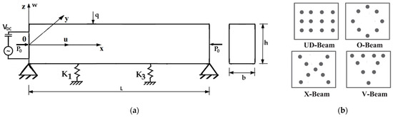
Figure 1.
The model of the CNTRC beam: (a) geometry of the CNTRC beam on an elastic foundation; (b) cross-section for different models of reinforcements.
A straight CNTRC beam made of a mixture of SWCNT and an isotropic polymer matrix was simply supported with the length L, thickness h, and width b. The beam was assumed to be immovable at both ends and had different models of reinforcement over the cross-sections, as presented in Figure 1b: uniform distribution (UD), O-distribution, X-distribution, and V-distribution. The material properties of the CNTRC beam were estimated by means of the rule of mixtures. The Young’s modulus, shear modulus G, Poisson’s ratio υ, and density ρ of the CNTRC were defined as follows [3,22,24]:
where superscripts CNT and p symbolize the related material properties of the carbon nanotube and polymer matrix, respectively; ηi, i = 1, 2, 3 indicates the efficiency parameters of CNT; and VCNT, and Vp are the volume fractions for the CNT and polymer matrix, respectively. , , and are the Young’s modulus and shear modulus of SWCNT, respectively; and are the corresponding material properties of the polymer matrix; and , , , and are the Poisson ratios and density of the CNT and polymer matrix, respectively.
The continuous mathematical functions utilized for describing the distributions of material constituents are presented as follows [22,24]:
in which z is the distance of any point on the physical middle surface along the thickness direction and z [−h/2, h/2], and:
where is the mass fraction of CNT. The CNT efficiency parameters ηi associated with the volume fraction are [3,22]:
3. Governing Equations of CNTRC Beams
The present research may shed light on the coupling effect of the thickness and shear deformation of CNTRC, so the unified beam theory was exploited in the beam’s modeling. A unified higher-order shear deformation beam theory incorporating various beam theories was used to capture the shear deformation and rotation. Within the framework of higher-order beam theory, the deformations of the beam took place in the x- and z-directions. According to the shear deformation theory, the displacement field consisting of the axial displacement U1 and the transverse displacement U3, at any point, is as follows [3,6,13,16,24]:
where the prime denotes the derivative with respect to variable x; u(x,t) and w(x,t) are the axial and transverse displacements at the reference plane of the beam, respectively; θ(x,t) is the bending rotation of the cross-section at any point of the reference plane; and t is the time. The shape function H(z) describes the transverse shear stress distribution across the beam thickness. Some of these shape functions for different beam theories are:
The expressions of the normal and shear strain components associated with the displacement field in Equations (13)–(15) are:
where the strain of the beam caused by the axial displacement ε1 is given by:
and the strain caused by the curvature is:
such that the normal strain component (17) becomes:
where
The shear strain becomes:
Now, based on the constitutive relation of the kth layer of the fiber-reinforced polymeric material, we obtain the stress:
where are transformed elastic constants in the z-direction defined by:
where φ is the direction of magnetic anisotropy; υ12 and υ21 are Poisson ratios; and G12, G13, G31, and G23 are the shear moduli.
3.1. Nonlocal Strain Gradient Theory
The total stress of the beam is defined as follows:
where is the differential operator, and and are the nonlocal stress and the higher-order nonlocal stress, respectively, expressed as:
where E is Young’s modulus, lm is the material length scale parameter or the strain gradient length scale parameter, εxx is the strain, εxx,x is the strain gradient, and are two nonlocal kernel functions satisfying Eringen conditions, and and are two nonlocal parameters. Having in view Equation (27), the one-dimensional problem of NSGT can be written as:
in which is the Laplace operator. For the particular case e0 = e1 = e, Equation (30) becomes:
For lm = 0, the last equation can be rewritten in the form:
which is the nonlocal constitutive equation for the nonlocal elasticity theory.
3.2. The Governing Equation for CNTRCs Considering the Thickness Effect
According to [30], by considering the thickness effect in the composite beam, the total stress can be expressed as:
where is the nonlocal stress, and and are higher-order nonlocal stresses.
The virtual strain energy is:
By substituting Equation (36) into Equation (34), after some manipulations, it holds that:
The virtual kinetic energy of CNT is given by:
where the dot denotes the derivative with respect to time.
Let
Taking into account Equations (13), (15), (21), and (39), the virtual kinetic energy becomes:
The virtual potential energy is given by the electromagnetic actuator, the nonlinear elastic Winkler–Pasternak foundation, the mechanical impact, and the compressive force P:
where C0, Vx, d, K1, K3, and F0 are capacitances of the actuator, voltage, the gap width, linear and nonlinear coefficients of the Winkler–Pasternak elastic foundation, and amplitude of the load, and is the delta-Dirac function.
The expression of the electromagnetic actuator can be simplified as:
The maximum error between the left and right expressions from Equation (42) was 3.3 × 10⁻⁶ for w/d [0, 0.15].
In this manner, the virtual work is given by:
where having considered the identity:
one gets:
Now, applying the Hamilton principle:
the governing equations of motion are obtained as:
Using the notations:
from Equations (32) and (47), we can obtain:
where f is given in Equation (21).
If the inertial axial moments are assumed to be negligible (I1 = I3 ≈ 0), and since the considered end supports of the composite beam are immovable: , , from Equations (47) and (51), we can get:
or in equivalent form:
For and , from the last equation, it holds that:
For the composite beam considered here, the boundary conditions for the simply supported beam are w(x) = w″(x) = 0 for x = 0 and x = L, such that Equation (54) becomes:
From Equations (31), (35) and (51), we can obtain:
For convenience, the following dimensionless variables were introduced:
Here, I0 and A110 are I0 and A11, respectively, for the homogeneous beam.
In what follows, the bar will be omitted. From Equations (56)–(58), we obtain:
The governing Equations (48) and (49) can be rewritten as follows:
where the functions g(x,t) and h(x,t) are given by Equation (21). The coefficients of B11, D11, and E11 are shown in Appendix A.
These nonlinear differential equations were very difficult to solve to obtain an exact solution.
The classical and nonclassical boundary conditions for a simply supported beam are:
We applied the Galerkin–Bubnov method to convert partial differential Equations (62) and (63) into an ordinary differential one. The displacement functions were assumed to have the form:
in which T1(t) and T2(t) are unknown, time-dependent functions and need to be determined, and and are a set of trial functions satisfying the boundary conditions.
Substituting expressions of g(x,t) and h(x,t) from Equation (21) into Equations (62) and (63), multiplying Equation (62) by sinπx and Equation (63) by cosπx, and integrating over domain [0,1], the following equations were yielded:
where the coefficients that appeared in these equations are shown in Appendix B.
The initial conditions for the system of (66) and (67) were:
For the simply supported beam, the shape functions can be chosen as:
The nonlinear differential Equations (66) and (67) were difficult to be analytically solved by exact solution, but a very accurate analytical solution can be found by means of OAFM [31,32,33,34,35].
4. The Optimal Auxiliary Functions Method
Let us consider a general form of nonlinear differential equations and boundary conditions:
where in the last two equations, L, N, t, T(t), D, and B are the linear operator, nonlinear operator, time, the unknown function of time, the domain of interest, and the boundary operator, respectively. According to OAFM, an approximate solution of Equations (69) and (70), , has only two components:
where n is an arbitrary integer number, and C1, C2, …, Cn are unknown parameters.
The initial approximation can be obtained from the linear equation:
In general, the solution of this equation has the form:
where the coefficients Ki, the functions fi, and the integer number m are known by elementary calculations. The nonlinear operator N from Equation (69) calculated for the value of and given by Equation (73) may be easily written in the form:
where the coefficients pi, the function gi, and the integer number m1 are known.
With the help of the method of influence function, operator method, and Cauchy method, we considered the unknown first approximation as the solution of the linear differential equation:
in which Ck represents n unknown parameters, and Fk represents the “auxiliary functions” depending on only some functions, fi and gj, involved in Equations (73) and (74). More precisely, the auxiliary functions Fk are combinations of known functions fi and gj. We noticed that we had the freedom to choose the values of the integer n and of the auxiliary functions Fk [31].
It is clear from Equation (71) that the boundary conditions were fulfilled, and Equation (69) responded to all initial/boundary conditions. Following our technique, the parameters Ck, were optimally identified by some known procedures, such as the Ritz method, the Galerkin method, the least squares method, the Kantorovich method, and the collocation method, or by minimizing the square residual error.
In this way, the auxiliary functions Fk, the parameters Ck, and analytical solution were known. It was remarkable that if the number of the convergence-control parameters increased, then the accuracy of the results obtained by our procedure grew. Finally, we can emphasize that any nonlinear differential equation can be reduced to only two linear differential equations, and OAFM does not suppose the presence of small parameters in the governing equations or in the initial/boundary conditions.
5. OAFM for Nonlinear Vibration of CNTRC
If we introduce the notations:
then the nonlinear differential Equations (66)–(68) can be rewritten in the equivalent forms:
in which ϖ1 and ϖ2 are unknown frequencies of T1 and T2, respectively.
The linear and nonlinear operators of Equations (77) and (78) are, respectively:
with the initial conditions:
The approximate solutions of Equations (77) and (78) are, respectively:
The initial approximations T10 and T20 are obtained from the linear equations:
whose solutions are, respectively:
The expression of the nonlinear operator given by Equation (79) calculated for the values given by Equation (85) becomes:
or
where
The first approximation can be obtained from Equation (75):
However, as we mentioned before, this choice of auxiliary functions was not unique. Also, the first approximation can be obtained from the following equations:
or
In what follows, we considered only Equation (89), whose solution is:
The approximate solution of Equation (77) is obtained from Equations (82), (85), and (92):
In the same way, the approximate solution of Equation (78) can be chosen in the form:
and the unknown convergence-control parameters can be obtained by means of a collocation approach.
The accuracy of our procedure was assured by comparing the results obtained by OAFM and numerical integration results.
6. Numerical Example
We illustrated the efficiency, accuracy, and applicability of our procedure by comparing the approximate solutions given by Equations (93) and (94), with the results obtained numerically by means of a fourth-order Runge–Kutta method. For the coefficients of Equations (77) and (78) given in Appendix B, we had the dimensionless parameters: m2 = 0.0215; m3 = 0.00054; a1 = 2.161; a2 = 0.0341; a3 = −0.000024; a4 = 0.53; b3 = 0.014; b4 = 0.4; b5 = 0.433; b6 = 0.0052; and b7 = 0.338.
The convergence-control parameters and the frequencies were:
To validate the present results obtained with OAFM, in Figure 2, we illustrated a comparison between analytical approximate solutions (93) and (94) and the numerical solution.
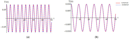
Figure 2.
Comparison between the approximate solution and numerical solution: (a) approximate solution (93); (b) approximate solution (94).
In another case, considering an increased value of the parameter b5 from b5 = 0.433 to b5 = 0.52, we obtained the convergence-control parameters: C1 = −0.0000252435, C2 = −0.0000581228, C3 = 0.0000142428, C4 = −0.000268119, C5 = 0.0000548702, C6 = −0.0000177365, C7 = −9.70021 × 10⁻⁸, C8 = −0.0000102798, and C9 = 1.59806 × 10⁻⁶, and the obtained approximate solutions are presented in Figure 3, in comparison with numerical integration results.
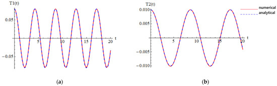
Figure 3.
Comparison between the approximate solution and numerical solution in the second case: (a) approximate solution (93); (b) approximate solution (94).
It is easy to observe that our approximate solutions of CNT were nearly identical to the numerical integration results, which proved the efficiency of our technique. The maximum errors between solutions (93) and (94) and the numerical results were 0.113% and 0.093%, respectively.
7. Buckling Analysis
For the buckling analysis, we ignored the kinematic terms in Equations (61) and (62) and the transverse distributed force q. To these new equations, we associated a homotopy, introducing so-called embedding parameter p, as shown in the following. Equations (61) and (62), ignoring the derivative with respect to time and force q, can be rewritten in the form:
where L and N are the linear and nonlinear parts, respectively, of these new equations.
Using the homotopy technique, we constructed a homotopy , which satisfied [36,37]:
where p [0,1]. It was obvious that when p = 0, Equation (97) became a linear equation; when p = 1, it became the original nonlinear one (96). The basic assumption was that the solution of Equation (96) can be written as a power series of p:
Setting p = 1 resulted in the approximate solution of Equation (96):
Following this approach, called the Homotopy Perturbation Method (HPM), the construction of the homotopy for Equations (61) and (62), without the terms in time and using the expressions (21) and (63) for the functions g and h, is shown in Appendix B.
To solve these equations, according to HPM, we searched for the solutions:
Inserting Equation (104) into (102) and (103) and then identifying the coefficients of pi, i = 0, 1, 2, we obtained the following equations:
Taking into account the boundary conditions for the simply supported CNTRC and using the Galerkin weighted residual method for Equations (105) and (106), the solutions were of the form:
in which A0 and B0 are unknown parameters, such that one can get:
where A0 is unknown at this moment.
For Equations (109) and (110), we proposed the solutions:
such that we found:
In the same way, identifying the coefficients of p2 into Equations (101) and (103), for:
we found that:
From Equations (104), (107) and (116), it holds that:
It is very important to mention that the values of the parameters A0, A1, and A2 were determined optimally, such that errors between the numerical solution of Equations (102) and (103) for the embedding parameter p = 1 and the approximate solutions (116) and (117) were minimum for the different types of CNTRC.
8. Bending Analysis
For bending analysis, kinematic terms and axial compression load P0 were ignored. We determined the static load-maximum deflection relationship, assuming that the transverse load q was constant. In this case, the corresponding homotopy can be written as:
For the bending analysis, we considered that:
Inserting Equation (121) into (119) and (120) and identifying the coefficients of pi, i = 0, 1, 2 in the same manner as the above section, we can see that Equations (105) and (110) were unchanged, such that the solutions:
led to the conclusions:
The Equation (105) can be rewritten as:
It follows that:
After some calculations, similarly to the previous section, from the coefficients of p1 and p2, for the values of V0, V1, V3, η0, η1, and η2, one can get:
Finally, from Equations (122)–(129), it holds that:
in which , , and were determined optimally as in the previous section.
9. Numerical Results and Discussion
The results obtained in the previous section, for different particular cases, such as the strain (shear and normal), the curvature, material length scale parameters, nonlocal parameter ratio (ea), the volume fraction parameter VCNT, and so on, were compared with several numerical examples available in scientific literature for the simply supported CNTRC nanobeams, with or without NSGT.
9.1. Buckling
In the following, we considered the values of the parameters [19] ea = l = 1 nm, L/h = 10, b = h = 5 mm, E = 210 × 109, and V = 0.24. In Figure 4, the dimensionless buckling load with respect to the small-scale parameter ea is depicted, where the solid line was plotted based on data from [13], and the dashed line was plotted based on present results.
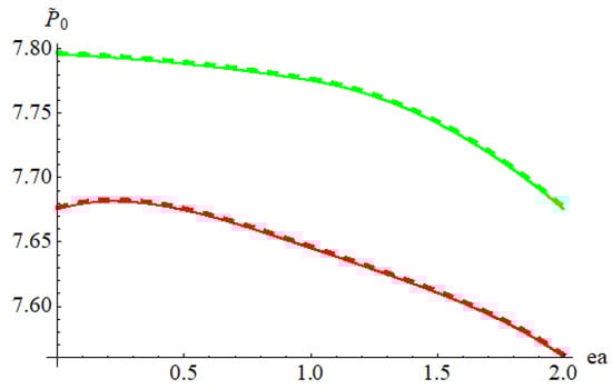
Figure 4.
Dimensionless buckling load for Euler–Bernoulli (green) and Timoshenko beams (red), with respect to small-scale parameter ea, for E = 210 × 109, υ = 0.24, h = b = 5 nm, and L = 100 h.
It can be seen that the dimensionless buckling load decreased once the small-scale parameter increased.
The buckling load for the Euler–Bernoulli beam was higher than the buckling load for the Timoshenko beam. On the other hand, the results obtained in this paper were nearly identical to the results presented in [13]. (The maximum difference was 0.73%).
Figure 5 shows the influence of the slenderness ratio (L/h) on the dimensionless buckling loads for a simply supported CNTRC nanobeam for l = 1, h = 1 nm, υ = 0.3, and and for the three cases: ea = 1/2 (red), ea = 1 (green), and ea = 2 (blue), where the solid line was plotted based on data from [6], and the dashed line was plotted based on present results.
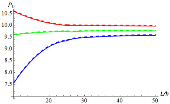
Figure 5.
Dimensionless buckling load with respect to slenderness ratio for l = 1. Effect of nonlocal parameter ea for E = 210 × 109, υ = 0.24, h = b = 5 nm, and L = 100h: ea = 1/2 (red), ea = 1 (green), and ea = 2 (blue).
It was observed that the dimensionless buckling load was lower than the ones given by classical theory (l = ea), when l < ea. If l > ea, then the dimensionless buckling load was higher than the ones given by classical theory. Also, for l < ea, the dimensionless buckling load increased with the increasing of the slenderness ratio, and for l > ea, the dimensionless buckling load decreased with the increasing of the slenderness ratio. An excellent agreement was observed between the results obtained in this paper and results obtained in [6]. (The maximum difference was 0.302%.) We remark that for l < ea, the nanobeam was softened, while for l > ea, the nanobeam was hardened, becoming easy to deform; also, the size effects were more significant for the lower values of the slenderness ratio (L/h < 30).
In Figure 6, the variation of the dimensionless buckling load is presented with respect to the slenderness ratio for UD-beam (green), X-beam (red), and O-beam (blue) for nm and b = h, where the solid line was plotted based on data from [10], and the dashed line was plotted based on present results.
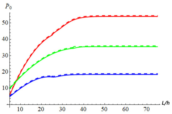
Figure 6.
Variation of the dimensionless buckling load with respect to the slenderness ratio for b/h = 1, l = 0.2, and VCNT = 0.12 for different distribution forms: X-beam (red), UD-beam (green), and O-beam (blue).
It was clear that if L/h increased, then the values of the dimensionless buckling loads increased at the beginning, and finally, it stabilized at a constant value corresponding to the known results of the Euler–Bernoulli beam [10].
In Table 1, the normalized buckling load of the CNTRC nanobeam is presented for the classical theory (ea = 0) and nonlocal theory for and for different values of the volume fraction parameter VCNT. From Table 1, we can deduce that the results obtained by classical theory for the buckling values were higher than the results obtained for nonlocal theories. Also, if the nonlocal parameter ea increased, then the values of the normalized buckling load decreased. The highest increase in the normalized buckling loads was more pronounced in the X-beam in comparison with the UD-beam and O-beam.

Table 1.
The normalized buckling loads for different values of the volume fraction parameter.
In the particular case of the Timoshenko beam, for L/h = 15, the present solution based on NSGT agreed with the buckling results presented in [3,38], as shown in Table 2.
Table 2.
Comparison of critical buckling values of the CNTRC Timoshenko nanobeam for classical theory.
From Table 2, it followed that the values of the critical buckling load for the CNTRC Timoshenko beam increased, while the volume fraction parameter VCNT for any type of beam decreased.
The effects of the nonlocal parameter (ea), the material length scale parameter (l), and the slenderness ratio L/h for Euler–Bernoulli and Timoshenko beams on the critical buckling loads are presented in Table 3.
Table 3.
Comparison of critical buckling loads for CNTR, Euler–Bernoulli beam, and Timoshenko beam for different values of ea, l, and L/h.
From Table 3, by comparing the results obtained in [6] and the present work, we deduced that the critical buckling loads increased if the nonlocal parameter l increased, while the critical buckling load increased if the nonlocal parameter ea increased. Also, it was clear that the difference between the critical buckling loads of the Euler–Bernoulli beam and the Timoshenko beam was insignificant.
In all cases, the values of critical buckling loads for the nonlinear case were higher in comparison to the values of critical buckling loads for the linear case, accounting for the same type of nanobeam.
9.2. Bending
The bending behavior of a simply supported CNTRC nanobeam was investigated for various cases and compared with the results known in literature.
In Figure 7, dimensionless deflections were depicted for l = 1 for different values of the nonlocal parameter ea, ea = 2 (red), ea = 1 (blue), and ea = 1/2 (green), where the solid line was plotted based on data from [6], and the dashed line was plotted based on present results.
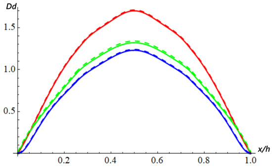
Figure 7.
Dimensionless deflection with respect to variable x/L for L/h = 10 and for the simply supported nanobeam: l = 1, ea = 2 (red), ea = 1 (blue), and ea = 1/2 (green).
It was observed that if l < ea, then the dimensionless deflection was higher than the dimensionless deflection obtained by classical theory (l = ea = 1), and vice versa for l > ea, the dimensionless deflection corresponded to the classical case. We observed that if the material length scale parameter l was smaller than the nonlocal parameter ea, the CNTRC nanobeam exhibited a stiffness-softening effect [6]. Considering Figure 6, the error for the case ea = 2 was 1.071%, ea = 1 was 0.871%, and ea = 1/2 was 0.698%.
In Table 4, the maximum normalized deflection CNRT nanobeam for data given in [10] is presented: L/h = 10, b = 4 m, and K1 = 0.1 for the uniform load and nonlocal parameter nm, with respect to some values of the volume fraction parameter VCNT. We deduced that if the values of the parameters VCNT increased, then the maximum deflection of a simply supported CNTRC nanobeam decreased, and our results were nearly identical to results obtained in [10]. The obtained results were very close to those presented in [10], being the maximum deviation observed, 0.667%. This result also showed that by increasing VCNT, the deflection of simply supported CNTRC nanobeams decreased.
Table 4.
The maximum normalized buckling loads for different values of the volume fraction parameter.
Table 5 presents dimensionless displacements of the UD-beam [3] without NSGT by varying the slenderness ratio L/h and volume fraction coefficient VCNT. It can be seen that if the slenderness ratio and volume fraction coefficient increased, then the dimensionless displacement decreased. Additionally, if the volume fraction coefficient was fixed, then if the slenderness ration increased, the dimensionless displacement decreased.
Table 5.
Dimensionless displacements without NSGT for uniform beam.
Table 6 presents the dimensionless maximum deflection for various values of the nonlocal parameter ea, material length parameter l, and slenderness ratio L/h for the Euler–Bernoulli beam and Timoshenko CNTRC nanobeam.
Table 6.
Comparison of dimensionless maximum deflection for CNTR, Euler–Bernoulli beam, and Timoshenko beam for different values of ea, l, and L/h.
Table 7 presents the errors and percentages comparing results known in literature and results obtained in this work, ; , where Rk represents results known in literature.
Table 7.
The errors and percentages for the results obtained in Table 1.
From Table 7, we can conclude that the results obtained in the present work for different cases were in very good agreement with the results obtained in literature. Additionally, from Table 1, Table 2 and Table 3, it is clear that the results obtained using our procedure for the nonlinear cases were substantially different when comparing the results with those obtained for linear cases.
We observed that the dimensionless maximum deflection of the Euler–Bernoulli beam was lower in comparison with the Timoshenko beam. Additionally, it can be seen that if ea increased, then dimensionless maximum deflection decreased, and if l increased and ea was unchanged, then the dimensionless maximum deflection decreased. On the other hand, if the slenderness ratio increased, then the values of the dimensionless maximum deflections for the Euler–Bernoulli beam and Timoshenko beam were close. The maximum error of the maximum deflection in Table 6 was 0.44% for the Euler–Bernoulli beam for L/h = 10 and l = 2 nm.
10. Conclusions
The present research deals with a comprehensive analysis of the nonlinear vibration of CNTRC nanobeams subjected to an electromagnetic actuator, mechanical impact, and nonlinear Winkler–Pasternak foundation. A generalized nonlocal beam theory according to the Eringen condition was used, and a higher-order shear deformation beam theory was applied to some types of beams, including Euler–Bernoulli and Timoshenko beams, as a special case in the present formulation, accounting for NSGT. The mechanical impact was especially considered for small load lengths.
To the best of the authors’ knowledge, no study has been conducted to account for the extension of normal and shear strain components with a generalized curvature in the presence of the nonlinear forces mentioned above. The governing equations were obtained based on the von Karman theory and then on the Hamilton principle.
Any system with infinite degrees of freedom was discretized by the Galerkin–Bubnov technique, and then the ordinary differential equations were solved by the Optimal Auxiliary Functions Method, even if the small parameter did not appear in the governing equations or in the initial/boundary conditions. It should be emphasized that the presence of a so-called auxiliary function, according to some theories about differential equations (operator method, Cauchy method, the method of influence functions), implies a rapid convergence of the approximate solutions using only the first iteration. The solutions obtained by the Optimal Auxiliary Functions Method were validated by comparisons with the numerical results gained using a fourth-order Runge–Kutta procedure.
Analytical solutions for critical buckling and the maximum deflection problems were studied by applying HPM, the Galerkin method in combination with the weighted residual method, and finally, by the optimization of results for simply supported composite nanobeams. Effects of nonlocality and length were investigated for some particular cases, as well as the influence of parameters, such as the volume fraction of CNTRC or size dependency for inhomogeneous or homogeneous nanobeam models.
Table 1, Table 2, Table 3, Table 4, Table 5 and Table 6 present some quantitative results obtained using OAFM, HPM, and Galerkin methods in comparison with the weighted residual method, and we compared them with those known in literature. Also, in Table 7, the errors and percentages were given corresponding to the presented results.
The main novelties in this work were represented by:
- -
- Extension of normal and shear strain;
- -
- A generalized curvature;
- -
- Introduction of the functions f(x,t), g(x,t), and h(x,t);
- -
- Combination between the electromagnetic actuator, nonlinear elastic Winkler–Pasternak foundation, and mechanical impact;
- -
- The Optimal Auxiliary Functions Method;
- -
- Study of buckling and bending using Homotopy Perturbation Method in combination with the Galerkin method and then the optimization method.
The obtained results were discussed and compared with the available results from literature. For different values of the nonlocal parameters, the dominated parameter can determine the stiffness-hardening or stiffness-softening effect on the CNTRC beam. The results obtained by our procedures were almost the same for the linear cases as those known, but the results of nonlinear cases were substantially different in comparison with the results obtained for the linear cases. The new results stress the necessity to include and consider complex nonlinear effects in the analysis of nanobeams subjected to electromagnetic actuators and mechanical impact.
Author Contributions
Conceptualization, V.M. and N.H.; methodology, V.M. and N.H.; software, B.M.; validation, N.H. and B.M.; formal analysis, V.M.; investigation, V.M. and N.H.; resources, N.H.; data curation, B.M.; writing—original draft preparation, V.M. and N.H.; writing—review and editing, V.M. and N.H.; visualization, B.M.; supervision, N.H. project administration, N.H. funding acquisition, N.H. All authors have read and agreed to the published version of the manuscript.
Funding
This research received no external funding.
Institutional Review Board Statement
Not applicable.
Informed Consent Statement
Not applicable.
Data Availability Statement
Data is contained within the article.
Conflicts of Interest
The authors declare no conflicts of interest.
Abbreviations
The following abbreviations are used in this manuscript:
| CNTs | Carbon nanotubes |
| NSGT | Nonlocal strain gradient theory |
| OAFM | Optimal Auxiliary Functions Method |
| HPM | Homotopy Perturbation Method |
| CNTRC | Carbon nanotube-reinforced beam |
| SWCNT | Single-walled carbon nanotube |
| LCB | Laminated composite beam |
Appendix A
The coefficients of B11, D11, and E11 from Equations (56) and (61):
The coefficients of D11, E11, and A55 from Equation (62):
Appendix B
References
- Shen, H.S.; Zhang, C.L. Nonlocal beam model for nonlinear analysis of carbon nanotubes on elastomeric substrates. Comput. Mater. Sci. 2011, 50, 1022–1029. [Google Scholar] [CrossRef]
- Rafiee, M.; Yang, J.; Kitipornchai, S. Thermal bifurcation buckling of piezoelectric carbon nanotube reinforced composite beams. Comput. Math. Appl. 2013, 66, 1147–1160. [Google Scholar] [CrossRef]
- Wattanasakulpong, N.; Ungbhakorn, V. Analytical solutions for bending, buckling and vibration responses of carbon nanotube-reinforced composite beams resting on elastic foundation. Comput. Mater. Sci. 2013, 71, 201–208. [Google Scholar] [CrossRef]
- Asadi, H.; Aghdam, M.M. Large amplitude vibration and post-buckling analysis of variable cross-section composite beams on nonlinear elastic foundation. Int. J. Mech. Sci. 2014, 79, 47–55. [Google Scholar] [CrossRef]
- Bahmyari, E.; Mohebpour, S.R.; Malekzadeh, P. Vibration analysis of inclined laminated composite beams under moving distributed masses. Shock Vib. 2014, 2014, 75098. [Google Scholar] [CrossRef]
- Lu, L.; Guo, X.; Zhao, J. A unified nonlocal strain gradient model for nanobeams and the importance of higher order terms. Int. J. Eng. Sci. 2017, 119, 265–277. [Google Scholar] [CrossRef]
- Shi, Z.; Yao, X.; Pang, F.; Wang, Q. An exact solution for the free vibration analysis of functionally graded carbon-nanotube-reinforced compsite beams with arbitrary boundary conditions. Sci. Rep. 2017, 7, 10909. [Google Scholar]
- Ouakad, H.M.; El-Borgi, S.; Mousavi, S.M.; Friswell, M.L. Static and dynamic response of CNT nanobeam using nonlocal strain and velocity gradient theory. Appl. Math. Model. 2018, 62, 207–212. [Google Scholar] [CrossRef]
- Fan, J.; Huang, J. Haar wavelet method for nonlinear vibration of functionally graded CNT-reinforced composite beams resting on nonlinear elastic foundation in thermal environment. Shock Vib. 2018, 2018, 9597541. [Google Scholar] [CrossRef]
- Borjalilou, V.; Taati, E.; Tahmadian, M. Bending, buckling and free vibration of nonlocal FG-carbon nanotube-reinforced composite nanobeams: Exact solutions. SN Appl. Sci. 2019, 1, 1323. [Google Scholar] [CrossRef]
- Pourasghar, A.; Chen, Z. Nonlinear vibration and modal analysis of FG nanocomposite sandwich beams reinforced by aggregated CNTs. Polym. Eng. Sci. 2019, 59, 25119. [Google Scholar] [CrossRef]
- Wang, Y.; Xie, K.; Fu, T.; Shi, C. Bending and elastic vibration of a novel functionally graded polumer nanocomposite beam reinforced by graphene nanoplatelets. Nanomaterials 2019, 9, 1690. [Google Scholar] [CrossRef] [PubMed]
- Hashemian, M.; Foroutan, S.; Toghraie, D. Comprehensive beam models for buckling and bending behavior of simple nanobeam based on nonlocal strain gradient theory and surface effects. Mech. Mater. 2019, 139, 103209. [Google Scholar] [CrossRef]
- Shafiei, H.; Setoodeh, A.H. An analytical study of the nonlinear forced vibration of functionally graded carbon nanotube-reinforced composite beams on nonlinear viscoelastic foundation. Arch. Mech. 2020, 72, 81–107. [Google Scholar]
- Huang, K.; Cai, X.; Wang, M. Bernoulli-Euler beam theory of single-walled carbon nanotubes based on nonlinear stress-strain relationship. Mater. Res. Express 2020, 7, 125003. [Google Scholar] [CrossRef]
- Keshtegar, B.; Kolahchi, R.; Eyvaziah, A.; Trung, N.T. Dynamic stability analysis in hybrid nanocomposite polymer beams reinforced by carbon fibers and carbon nanotubes. Polymers 2021, 13, 106. [Google Scholar] [CrossRef]
- Su, Y.C.; Cho, T.Y. Free vibration of a single-walled carbon nanotube based on the nonlocal Timoshenko beam model. J. Mech. 2021, 37, 616–635. [Google Scholar] [CrossRef]
- Senthilkumar, V. Axial vibration of double-walled carbon nanotubes using double nanorod model with van der Waals force under Pasternak medium and magnetic effect. Vietnam J. Mech. 2022, 44, 29–43. [Google Scholar] [CrossRef]
- Zhao, J.L.; Chen, X.; She, O.L.; Jing, Y.; Bai, R.Q.; Yi, J.; Pu, H.Y.; Luo, J. Vibration characteristics of functionally graded carbon nanotube-reinforced composite double-beams in thermal environments. Steel Compos. Struct. 2022, 43, 797–808. [Google Scholar]
- Essen, I.; Tran, T.T.; Nguyen, D.K. Dynamic response of FG-CNTRC beams subjected to a moving mass. Vietnam J. Sci. Technol. 2022, 60, 853–868. [Google Scholar]
- Seyfi, A.; Teimouri, A.; Dimitri, R.; Tornabene, F. Dispersion of elastic waves in functionally graded CNTs-reinforced composite beams. Appl. Sci. 2022, 12, 3852. [Google Scholar] [CrossRef]
- Alimoradzadeh, M.; Akbas, S.D. Nonlinear oscillations of a composite microbeam reinforced with carbon nanotube based on the modified couple stress theory. Coupled Syst. Mech. 2022, 11, 485–504. [Google Scholar]
- Dang, V.H.; Nguyen, T.H. Buckling and nonlinear vibration of functionally graded porous micro-beam resting on elastic foundation. Mech. Adv. Comp. Struct. 2022, 9, 75–88. [Google Scholar]
- Eghbali, M.; Hosseini, S.A. On moving harmonic load and dynamic response of carbon nanotube-reinforced composite beams using higher-order shear deformation theories. Mech. Adv. Comp. Struct. 2023, 10, 257–270. [Google Scholar]
- Mohanty, A.P.; Das, P.; Choudhury, S.; Sanu, S.K. Free vibration behavior of laminated composite beam under crack effects. A combined numerical and experimental approach. Ann. Chim. Sci. Matériaux 2024, 48, 447–455. [Google Scholar] [CrossRef]
- Huang, Z.; Li, Y.; Cheng, Y.; Wang, X. Finite element modeling and vibration control of composite beams with partially covers active constrained layer damping. Sound Vib. 2025, 59, 1765. [Google Scholar] [CrossRef]
- Sharma, P.; Kumar, R.D.; Khinchi, A. Behavior of tri-directional advanced composite beams using finite element method. J. Polym. Comp. 2025, 13, 610–620. [Google Scholar]
- Murugan, H.; Ramamoorthy, M. Investigation of vibration-induced fatigue on composite sandwich beam with GFRP laminate and PLA honeycomb stiffened core. Mech. Based Struct. Mach. 2025, 53, 1–24. [Google Scholar] [CrossRef]
- Zhang, G.; Hao, Y.; Guo, Z.; Mi, C. A new model for thermal buckling of FG-MEE microbeams based on a non-classical third-order shear deformation beam theory. Mech. Solids 2024, 59, 1475–1495. [Google Scholar] [CrossRef]
- Li, L.; Tang, H.; Hu, Y. The effect of thickness on the mechanics of nanotubes. Int. J. Eng. Sci. 2017, 123, 81–91. [Google Scholar] [CrossRef]
- Marinca, V.; Herisanu, N. The nonlinear thermomechanical vibration of a functionally graded beam on Winkler-Pasternak foundation. MATEC Web Conf. 2018, 148, 13004. [Google Scholar] [CrossRef][Green Version]
- Herisanu, N.; Marinca, V. An effective analytical approach to nonlinear free vibration of elastically microtubes. Meccanica 2021, 561, 813–823. [Google Scholar] [CrossRef]
- Herisanu, N.; Marinca, B.M.; Marinca, V. Longitudinal–transverse vibration of a functionally graded nanobeam subjected to mechanical impact and electromagnetic actuation. Symmetry 2023, 15, 1376. [Google Scholar] [CrossRef]
- Herisanu, N.; Marinca, V.; Madescu, G. Application of the Optimal Auxiliary Function Method to a permanent magnet synchronous generator. Int. J. Nonlinear Sci. Numer. Simul. 2019, 20, 399–406. [Google Scholar] [CrossRef]
- Marinca, B.M.; Herisanu, N.; Marinca, V. Investigating nonlinear forced vibration of functionally graded nanobeam based on nonlocal strain gradient theory considering the mechanical impact, electromagnetic actuator, thickness effect and nonlinear foundation. Eur. J. Mech. A-Solids 2023, 102, 105119. [Google Scholar] [CrossRef]
- He, J.H. Some asymptotic methods for strongly nonlinear equations. Int. J. Mod. Phys. B 2006, 20, 1141–1199. [Google Scholar] [CrossRef]
- He, J.H. Homotopy perturbation method for solving boundary values problems. Phys. Lett. A 2006, 350, 87–88. [Google Scholar] [CrossRef]
- Yas, M.H.; Samadi, N. Free vibrations and buckling analysis of carbon nanotube-reinforced composite Timoshenko beams on elastic foundation. Int. J. Press. Vess. Pip. 2012, 98, 119–128. [Google Scholar] [CrossRef]


Disclaimer/Publisher’s Note: The statements, opinions and data contained in all publications are solely those of the individual author(s) and contributor(s) and not of MDPI and/or the editor(s). MDPI and/or the editor(s) disclaim responsibility for any injury to people or property resulting from any ideas, methods, instructions or products referred to in the content. |
© 2025 by the authors. Licensee MDPI, Basel, Switzerland. This article is an open access article distributed under the terms and conditions of the Creative Commons Attribution (CC BY) license (https://creativecommons.org/licenses/by/4.0/).