Dynamic Relevance-Weighting-Based Width-Adaptive Auto-Encoder

Abstract

This paper proposes a novel adaptive autoencoder model that autonomously determines the optimal latent width during training. Unlike traditional autoencoders with fixed architectures, the proposed method introduces a dynamic relevance weighting mechanism that assigns adaptive importance to each node in the hidden layer. This distinctive feature enables the simultaneous learning of both the model parameters and its structure. A newly formulated cost function governs this dual optimization, allowing the hidden layer to expand or contract based on the complexity of the input data. This adaptability results in a more compact and expressive latent representation, making the model particularly effective in handling diverse and complex recognition tasks. The originality of this work lies in its unsupervised, self-adjusting architecture that eliminates the need for manual design or pruning heuristics. The approach was rigorously evaluated on benchmark datasets (MNIST, CIFAR-10) and real-world datasets (Parkinson, Epilepsy), using classification accuracy and computational cost as key performance metrics. It demonstrates superior performance compared to state-of-the-art models in terms of accuracy and representational efficiency.

1. Introduction

Machine Learning (ML) is a field of Artificial Intelligence (AI) which involves exploiting available data and devising algorithms to emulate human learning. Recently, the Deep Learning (DL) paradigm has added a conceptual and an algorithmic cutting edge to the machine learning field [1,2]. As such, it has accomplished great success in various fields such as image classification [3], anomaly detection [4], object detection [5], pattern recognition [6], and natural language processing [7], etc. The successful performance of these models is mainly due to the automatic learning of the features from raw data. For instance, Convolutional Neural Networks (CNN) [1] have been exploited broadly for image classification problems [3], and Recurrent Neural networks (RNN) [1] have been employed for sequential data classification such as videos or speech. Alternatively, Autoencoders (AEs) [1] are unsupervised deep learning paradigms, and have been proven to be effective for dimensionality reduction, feature mapping, anomaly detection, image denoising, hyperspectral unmixing, and image generation [1]. Consequently, they have been adopted in many fields such as bioinformatics [8], recommender systems [9], remote sensing [10], and cybersecurity [11]. Moreover, they constitute a main component in successful NLP transformers’ architecture, such as Google’s BERT [12] and OpenAI’s GPT [13].

The greatest challenge when dealing with AEs is choosing the best topology that produces a meaningful and generalizable latent space representation. Typically, the depth and the width hyperparameters control the topology of a stacked autoencoder and thus affect its performance [14]. Specifically, the depth specifies the number of stacked autoencoders, i.e., the depth of the network, whereas the width specifies the number of hidden units with respect to each layer. The latter corresponds to the number of nodes in the case of a fully connected AE.

Determining the most effective topology of an autoencoder (AE) by tuning its depth and width is a challenging task, particularly in unsupervised settings where labeled data are often unavailable for performance evaluation. However, studies such as [14,15] have shown that even simple architectures with a single hidden layer can achieve state-of-the-art performance when the width is appropriately configured. These findings highlight that the width of an AE can be more influential than its depth in attaining high performance. Consequently, rather than relying on stacked AEs with multiple layers, it becomes essential to identify the optimal number of neurons in the hidden layer of a fully connected AE. Moreover, optimizing width over depth enhances computational efficiency, as wider architectures can leverage parallel matrix operations, whereas deeper networks involve sequential computations. Deep architectures are also more susceptible to challenges such as overfitting [1] and the vanishing gradient problem [2], further supporting the emphasis on width in AE design. Nevertheless, selecting the ideal width remains non-trivial. This is because the width must be defined per dataset and is highly sensitive to data complexity, structure, and noise levels—creating a need for a principled and data-driven approach to determining the latent width rather than relying on arbitrary or fixed configurations.

One way of tackling the problem of setting the width of an AE is by empirical experimentation. Nonetheless, manual tuning of the width in such a large search space is computationally expensive and impractical. Moreover, determining the topology of an AE has attracted little attention compared to Supervised Artificial Neural Networks (ANN). In particular, previous attempts were mainly based on genetic and evolutionary optimization approaches, exhibiting expensive computational complexity [16]. This compels the creation of constrained topologies in which the number of nodes is limited [17]. Other alternatives append the AE with a classifier to benefit from the labeled data. Nonetheless, they compromise the unsupervised nature of AEs. This introduces a fundamental dilemma: while AEs are designed to learn from unlabeled data, many of the methods for selecting their structure assume the availability of labels. This contradicts the core unsupervised learning principle and highlights a significant gap in AE design, motivating our work to address this unresolved challenge.

In this paper, we propose to learn dynamically the width of an AE while training it. Specifically, we design a new cost function to optimize the relevance weight of each node and then learn the number of nodes of the hidden layer in the case of a fully connected AE. This optimization is achieved by assessing the inner product between the input vector and the mapped vector at each layer. The proposed approach involves the removal of non-relevant nodes, followed by an update to the AE architecture to reflect these changes. This method provides a fully unsupervised, self-adaptive mechanism that eliminates the need for manual tuning or auxiliary classifiers, thus preserving the integrity of unsupervised learning while improving architectural efficiency.

In summary, our contributions are threefold: (i) we propose a novel relevance-weight-based mechanism for dynamically adjusting the width of autoencoders during training; (ii) we formulate a new cost function based on inner-product preservation to guide node importance estimation; and (iii) we validate the method on both benchmark and real-world datasets, showing significant improvements over state-of-the-art fixed-structure and evolving models.

The rest of the paper is organized as follows: Section 2 reviews related work and theoretical foundations. Section 3 presents our proposed Width-Adaptive Autoencoder (WAAE) method. Section 4 details the experimental setup, including datasets and evaluation metrics. Moreover, it presents the results and analysis, while Section 5 concludes the paper and discusses limitations and future directions.

2. Literature Review

Due to its effect on the performance of the AE, learning the topology of an AE has recently gained interest among researchers. In particular, the width of the AE is estimated by pruning or adding neurons during the training phase. These models are known as dynamic, adaptive, or evolving AE models. They fall into two main paradigms, namely the supervised and the unsupervised paradigms. Supervised AEs employ a soft-max layer to benefit from the classification performance to assess the features map produced by the AE model. Alternatively, the unsupervised approach is based on the reconstruction error.

2.1. Supervised Learning Techniques

The Deep Evolving Denoising Auto-Encoder (DEVDAN) [18] learns the width of an AE based on Network Significance (NS). It is a supervised approach that utilizes a prequential test-then-train strategy. First, discriminative testing is performed to assess the generalization performance. For this purpose, a soft-max layer is appended to the DAE. Then, the network parameters are updated during the generative training phase. Based on that, the discriminative training is conducted. The estimation of NS is based on the approximation of the bias and the variance of the encoder–decoder model by calculating the squared reconstruction error and the expectation of the reconstructed input attributes z. It is expressed as in (1):

$$NS=Bias{\left(z\right)}^2+Var\left(z\right)$$

(1)

A high variance of the NS value implies overfitting, whereas a high bias of the NS value indicates underfitting. In this regard, based on NS, the hidden nodes are dynamically generated and pruned. Specifically, if the NS bias is greater than the prespecified threshold, a new node is generated in the hidden layer of the network. On the other hand, if the NS variance is greater than the prespecified threshold, the node exhibiting the lowest Hidden Node Significance (HS) index is pruned. The latter reflects the contribution of a hidden node and its significance. Specifically, it calculates the average activation degree of the i-th hidden node over all possible data samples.

The work in [19] adopts an incremental feature learning approach. It adds and merges neurons to an AE architecture based on generative, discriminative, and hybrid training processes. The approach combines the generative loss ($L_{gen}$) and the discriminative loss ($L_{disc}$) in a hybrid objective function. Precisely, when the objective function value is larger than a predefined threshold, new neurons are added. This objective function is defined as in (2):

$$L(x, y)=L_{disc}(x,y)+\lambda L_{gen}\left(x\right)$$

(2)

where x is an input sample, y is a ground-truth label, $L_{disc}$ represents the average classification loss between the actual label (y) and the predicted label ($\tilde{y}$), and $L_{gen}$ represents the average reconstruction error between the input data (x) and the reconstructed data ($\tilde{x}$). Both losses are computed using cross-entropy function. The parameter λ controls the trade-off between the discriminative and generative objectives. The objective function is estimated after training a sub-set of the training instances. After adding new neurons, only these neurons with their corresponding parameters are trained. Nevertheless, adding too many neurons may result in overfitting. To counteract this issue, similar neurons are merged in order to produce compact feature representation. More precisely, neurons with minimal weight cosine distances are merged. The weights of the merged neurons are initialized with the average of their weights. They are then trained using the hybrid objective function (2). Finally, the generative process minimizes the reconstruction error, and the discriminative process minimizes the average classification error.

2.2. Unsupervised Learning Techniques

The width of a stacked fully connected AE is learned with respect to each layer by pruning irrelevant neurons in [20]. Irrelevant neurons are identified by comparing the neuron reconstruction error with a predefined threshold. The reconstruction error is a measure of how well a model can reconstruct the original input data from its encoded representation. It is used as a criterion for selecting the most informative features and pruning unnecessary units. Therefore, if the neuron reconstruction error is 20 times greater than the threshold, the related neuron and its input data is prohibited from participating in the training process. The performance evaluation is based on their ability to reconstruct the input data with the least amount of error.

In [17], the Neurogenesis Deep Learning (NDL) is introduced. It involves adding new neurons at any layer while training a stacked deep AE. Specifically, the reconstruction error (RE) is used to determine if an AE (pair of encode/decode layers) is able to represent that input set. In fact, If RE is higher than a predefined threshold, the AE does not have enough neurons to reconstruct the data. Therefore, a neuron is added to the AE under consideration. As such, neurons are incrementally added until the number of neurons reaches a maximum user-defined value. Consequently, NDL is trained with the whole training data when a new neuron is added. The process is repeated until the RE falls below the predefined threshold or when the maximum number of neurons for the current layer is reached.

Another study that used a bias–variance regulation method is the “Self-evolving Autoencoder Embedded Q-Network” (SAQN) [21], which is an innovative combination of self-adaptive autoencoders and reinforcement learning. The autoencoder progressively adapts as the agent engages with its surroundings. This versatility enables the autoencoder to proficiently capture a wide array of observations, expressing them effectively in its latent space. The evolution process involves node growth, integrating additional nodes to retain previously acquired knowledge, and ensuring a comprehensive representation of the environment. Node Pruning involves removing fewer contributory nodes to maintain a manageable and efficient latent space. This adaptive method ensures that the autoencoder remains responsive to new information while preserving essential knowledge. A core component of SAQN is the bias–variance regulation method, which balances the model’s complexity with generalization ability. This technique optimally adjusts the reinforcement learning agent’s response to environmental changes by regulating node growth and pruning. The SAQN adheres to the same bias–variance regulatory strategy as the DEVDAN [18] model. Nevertheless, DEVDAN employs discriminative and generative training, whereas SAQN exclusively employs generative training.

An evolutionary approach is used in [22] to learn AE architecture. The AE configuration is represented by a chromosome on which crossover and mutation operations are performed. Precisely, the chromosome is composed of a set of 14 genes organized into five groups. The first group consists of one gene to set the type of AE, the second group includes one gene to estimate the number of layers, the third group includes three genes to set the number of units per layer, the fourth group includes six genes to define the activation functions, and, lastly, the fifth group includes one gene to evaluate the loss function.

Another study [23] employs evolutionary search methodology to estimate the topology of an AE. However, the depth is constrained to five. Similarly, the width is constrained to be a multiple of 50 which is larger than 50, and smaller than 1000. The fitness function of the evolutionary search is defined as the inverse of the AE reconstruction loss. To optimize the fitness function, a mutation is applied on the parent genotype to give an offspring which increments the depth. Once the maximal depth is attained, the mutation is performed on the parent genotype to modify the width at random layers. All unsupervised approaches are based on the reconstruction error. This may lead to an overfitting problem since it is used for both the weight learning and topology learning.

2.3. Autoencoder Compression and Architectural Adaptability

Autoencoder compression and architectural adaptability have become prominent areas of research in light of the increasing computational demands and deployment challenges of deep neural networks. Our work builds upon and complements several major lines of research in model pruning, architectural adaptation, and width-scalable representations.

Recent advances in model compression and pruning have emphasized the importance of non-uniform and adaptive strategies. For instance, Shapley Value-based pruning [24] and dynamic structure pruning [25] allocate resources based on component significance rather than uniform heuristics. Methods such as AST [26] and LAASP [27] further integrate adaptive training or loss-aware criteria to balance efficiency and accuracy. These approaches are mainly designed for large-scale language models or CNNs. In contrast, our approach introduces a width-adaptive autoencoder architecture that dynamically scales its latent dimension based on node relevance during training, a principle not directly explored in the aforementioned studies.

Pruning is a widely used model compression technique that reduces parameter counts by eliminating unimportant weights or structures. Traditional pruning approaches often apply uniform sparsity across layers, which can lead to suboptimal performance. Recent methods have moved towards non-uniform and adaptive pruning strategies to better preserve task-critical parameters. For instance, Sun et al. [24] introduced a Shapley value-based non-uniform pruning approach for large language models (LLMs), assigning different sparsity levels to layers based on their importance. Their sliding-window-based approximation significantly improves computational efficiency while enhancing perplexity and accuracy compared to uniform pruning baselines like SparseGPT. Similarly, Huang et al. [26] proposed the Adaptive Sparse Trainer (AST), a semi-structured sparse training framework for LLMs that avoids the performance degradation common in one-shot pruning by integrating distillation and weight mask learning during training.

Other notable approaches, such as Malihi and Heidemann [28], combine knowledge distillation with pruning to achieve compact models without loss in accuracy. This synergy enhances the control over compression levels and yields strong generalization, demonstrated on ResNet and DenseNet architectures. The Reweighted ADMM method by Yuan et al. [29] presents another advancement, introducing a reweighting mechanism in the pruning process that outperforms traditional thresholding by dynamically adjusting weight importance. Additionally, Liu et al. [30] proposed IESSP, a sparse stripe pruning strategy that improves feature retention via a novel loss function and information extraction module, achieving substantial FLOP reductions without compromising accuracy.

From a structured pruning perspective, Ghimire et al. [31] developed a loss-aware automatic criterion selection technique that integrates pruning into training. By automating pruning decisions based on loss metrics, their method eliminates manual tuning and improves both accuracy and compression. Furthermore, Park et al. [25] proposed Dynamic Structure Pruning, which optimizes intra-channel pruning granularities during training using a differentiable group learning strategy, outperforming standard channel pruning in FLOPs and runtime acceleration. Finally, Zhao et al. [32] explored post-training pruning for foundation models, targeting both unstructured and semi-structured sparsity without retraining. Their algorithm achieves substantial compression while minimizing performance degradation, making it practical for deployment scenarios with limited computational resources.

Alongside pruning, researchers have explored architectural adaptation as a means to optimize network capacity dynamically. Elastic and Slimmable networks [33] enable runtime width adjustment, allowing a single network to operate at multiple capacity levels. Extensions such as Once-for-All networks [34] further support deployment across diverse hardware by learning multiple subnetworks in one training process.

2.4. Discussion

Despite recent progress in evolving architectures (DEVDAN [18], SAQN [21], and NDL [17]), most methods still rely on manual thresholding, fixed pruning schedules, or heuristic-based evaluations of node importance. These approaches often suffer from instability or lack of theoretical grounding. In contrast, our method introduces a continuous, relevance-weight-based adjustment guided by an inner-product-preserving objective, allowing both expansion and pruning without manual intervention. This positions our model as a principled and flexible alternative to existing fixed and evolving autoencoders.

Compared to prior work, our Width-Adaptive Autoencoder (WAAE) introduces a novel strategy to dynamically control the latent width during training. This offers a complementary mechanism to pruning; rather than removing weights post hoc, we proactively adapt the model architecture in response to training signals. Our method supports flexibility during inference and can match model capacity to resource constraints without separate retraining. Thus, our approach lies at the intersection of adaptive compression and architecture search, contributing a new dimension to model efficiency by enabling width-scalable representations in the autoencoder framework.

Unlike prior methods such as DEVDAN, SAQN, and NDL that rely on heuristic-based or threshold-driven pruning, our approach introduces a principled relevance-weighting mechanism based on an inner-product-preserving objective. This formulation allows for continuous and data-driven adaptation of network width, ensuring stable learning dynamics without reliance on empirical thresholds or task-specific tuning. As a result, our model offers a more generalizable and theoretically grounded framework for width-adaptive representation learning.

To ground our approach theoretically, we build on the principle of inner-product preservation as a mechanism for evaluating and maintaining the relevance of neurons during training. Specifically, we define a relevance score for each neuron based on its contribution to preserving the pairwise inner products of hidden representations, which are indicative of the local geometry of the feature space. This allows for a continuous, data-driven adaptation of network width, offering a principled alternative to discrete pruning heuristics or static architectural decisions commonly found in previous work.

3. Width-Adaptive Autoencoder

In this research, we propose a method to dynamically learn the optimal width of an autoencoder (AE) in an unsupervised manner during the training process. This results in an adaptive AE architecture that eliminates the need to manually specify the number of hidden layer neurons.

3.1. Motivation

The width of an autoencoder (AE) significantly influences its performance. Hence, determining the optimal number of nodes in the hidden layer of a fully connected AE is essential for achieving optimal results. In fact, insufficient neurons may prevent the AE from extracting the key characteristics of the data and reconstructing the learned representation at the output layer. On the other hand, if the width is too large the AE faces computational constraints [35] and may be prone to saturation. To motivate the proposed WAAE, we first evaluated conventional non-evolving autoencoders with manually fixed widths on MNIST [36] and CIFAR-10 [37] (see Figure 1). These experiments illustrate how performance is highly sensitive to the choice of width, requiring extensive tuning to identify optimal configurations. This analysis serves as a baseline comparison and justifies the need for an adaptive architecture that can learn the appropriate capacity during training. Specifically, the number of nodes is tuned from 100 to 5000. The AE is trained in an unsupervised manner, and its learned representations are subsequently evaluated by feeding them into a SoftMax classifier. The classification accuracy is then used to assess the influence of width on the overall performance. We should emphasize here that the SoftMax classifier is only employed for assessment purposes. It is not involved in any way in training the AE and in the adaptative learning of the width. Figure 1 shows the classifier’s accuracies with respect to different width values.

Figure 1a illustrates the effect of varying the hidden layer width on the classification accuracy for the MNIST dataset. As the number of neurons increases from 100 to 5000, the accuracy improves steadily, with a significant rise observed up to around 1000 neurons. Beyond this point, the performance continues to increase but at a slower rate, eventually stabilizing around 97%. This trend indicates that a wider autoencoder (AE) enables better representation learning for MNIST, a relatively simple and structured dataset. The results highlight that the width of the hidden layer plays a crucial role in enhancing the AE’s ability to extract meaningful features that support downstream classification tasks. In contrast, Figure 1b presents the results for the CIFAR-10 dataset, revealing a markedly different pattern. While the accuracy starts around 40% and slightly improves with increased width, the overall gains are marginal, with performance plateauing below 45%. The fluctuations across different widths suggest that increasing the hidden layer size does not lead to significant improvements for this more complex dataset.

The observations from the two figures support the claim that the width of an autoencoder (AE) significantly influences its performance. In the case of the MNIST dataset, increasing the number of hidden layer neurons leads to a notable improvement in classification accuracy, demonstrating that a wider AE can capture more informative representations. However, beyond a certain width, the performance gains begin to plateau, indicating the importance of identifying an optimal rather than maximal number of neurons. This confirms that selecting the appropriate width is essential for achieving optimal results. When the hidden layer is too narrow, the AE struggles to extract key features from the input data, as seen in the low accuracy scores at smaller widths. Conversely, while very wide AEs may achieve slightly better performance, they also introduce computational overhead and demonstrate diminishing returns, suggesting a saturation effect. The CIFAR-10 results further emphasize that increasing width does not guarantee better performance.

To further analyze the impact of width on the learned representation, an autoencoder with a hidden layer of 5000 neurons was trained in an unsupervised manner. After training, a subset of the encoded features was selected and sorted based on their variance across the dataset. Heatmaps were generated to visualize these features, where each row corresponds to a data instance and each column represents a feature. The color intensity in the heatmap indicates the magnitude of the feature values. The aim was to assess the activity and relevance of the encoded features, particularly to observe whether all 5000 nodes were contributing meaningful information.

This experiment provides visual evidence that supports the earlier claim regarding the importance of determining the optimal number of hidden nodes in an autoencoder. As shown in the heatmaps (Figure 2), a significant number of features exhibit zero or near-zero variance, indicating that these nodes are either inactive or contribute negligibly to the learned latent representation. This observation suggests that the autoencoder, when configured with 5000 hidden nodes, possesses excessive capacity, resulting in the learning of redundant or overlapping features. Specifically, Figure 2a,b illustrate the high-variance features that actively participate in encoding meaningful patterns, while Figure 2c,d highlight a large portion of nodes that remain unused or underutilized, as evidenced by their zero or near-zero variance. These results have several important implications. First, they empirically validate the hypothesis that overly wide autoencoders do not necessarily enhance performance and instead may waste computational resources. Second, they highlight the need for a principled approach to selecting or adapting the width of the hidden layer to avoid overparameterization. The saturation effect observed, where increasing the number of nodes fails to improve the representation, reinforces the motivation behind our proposed method. Therefore, this visual analysis of quantitative feature variance reinforces the idea that selecting an optimal width is crucial for both effective representation learning and computational efficiency.

3.2. Proposed Approach

We propose to learn the optimal AE width automatically. The cornerstone of learning the width is based on understanding the relevance weight of each node, n, for a fully connected layer design. The suggested approach considers a single-layer design for the AE, but dynamically adding then pruning width until it reaches an optimal architecture. Precisely, updating the relevance weight for each node is done iteratively at the end of each batch b. The basis of the strategy is the construction using a cost function distinct from the network’s lost function form. The novel cost function for a fully connected AE optimizes the relevance weight of each node by measuring the inner product between the input vector and the mapped vector at each layer.

The proposed training procedure, illustrated in Figure 3, consists of four main iterative steps. First, a batch b is processed to update the network parameters and learn the mapping of each node within its respective layer. Next, a relevance score is computed for each node, reflecting its contribution to the learned representation. In the third step, new nodes are incrementally added to the hidden layer until the first pruning condition is met. Finally, a pruning phase is performed, where nodes with low relevance scores are removed. Each of these steps is described in detail in the following sections.

Learning the Nodes’ Relevance Weights

To determine the optimal width of the autoencoder dynamically, we introduce a mechanism to assess and learn the relevance weight of each node. Specifically, for a given node n at layer l and training batch b, we define a relevance score RN (n, l, b) that quantifies the contribution of that node to the representation learning process. The central idea is to compare how well each node in the latent space preserves the pairwise relationships of the input data. We do this by designing a separate cost function $J_{FC}\left(l\right)$, optimized independently from the autoencoder’s reconstruction loss, to guide the learning of the relevance weights.

• Relevance-Based Cost Function

Let $x\left(i\right)$ and $x\left(j\right)$ be two input vectors from batch $b$, and let $x\prime \left(n, l, i, b\right)$ denote the activation of node n at layer l for input $\left(i\right)$. We measure the difference in inner products between the input space and the latent space as follows:

$${\left(x\left(i\right). x\left(j\right)-x^{\prime }\left(n, l, i, b\right). x^{\prime }\left(n, l, j, b\right)\right)}^2$$

(3)

This term captures how well the projection through node n preserves the original similarity between inputs i and j. Nodes that better preserve this relationship should be assigned higher relevance.

To learn the weights $RN\left(n,l,b\right)$, we define the following cost function:

$$J_{FC}(l)=\sum _b^{NB\left(b\right)}\sum _{i\in b}\sum _{j\in b}\sum _{n=1}^{NN(l,b)}{RN\left(n,l,b\right)}^q{\left(x\left(i\right).x\left(j\right)-x^{\prime }\left(n,l,i,b\right).x\prime (n,l,j,b)\right)}^2$$

(4)

subject to the constraint:

$$\sum _{n=1}^{NN(l,b)}RN\left(n,l,b\right)=1$$

(5)

where NB is the number of processed batches, $NN(l,b)$ is the number of nodes at layer l, at batch b, and $q>1$ is a hyperparameter that controls the sparsity or “fuzziness” of the relevance weights. Lower values of q promote smoother distributions, while higher values encourage sparsity. The cost function aims to allocate higher weights to nodes that better preserve the inner product structure of the input space.

• Optimization of Relevance Weights

To minimize $J_{FC}\left(l\right)$ under constraint (5), we apply the method of Lagrange multipliers. Solving for $RN\left(n,l,b\right)$, we obtain the following closed-form expression:

$$RN\left(n,l,b\right)={\displaystyle \frac{{\frac{1}{T\left(n,l,b\right)}}^{\frac{1}{q-1}}}{\sum _{n=1}^{NN(l,b)}{\frac{1}{T\left(n,l,b\right)}}^{\frac{1}{q-1}}}}$$

(6)

where $T\left(n,l,b\right)$ represents the accumulated squared deviation of inner product preservation for node n:

$$T\left(n,l,b\right)=\sum _b^{NB\left(b\right)}\sum _{i\in b}\sum _{j\in b}{\left(x\left(i\right).x\left(j\right)-x^{\prime }\left(n,l,i,b\right).x\prime (n,l,j,b)\right)}^2$$

(7)

Thus, nodes with smaller $T\left(n,l,b\right)$ values are those that best preserve input similarity and are assigned larger relevance weights.

• Interpretation and Utility

The learned relevance weights $RN\left(n,l,b\right)$ provide an interpretable measure of each node’s utility. In fact, a high weight means that the node meaningfully contributes to preserving structural information in the data. Alternatively, a low weight means that the node contributes little and can be considered for pruning. This process facilitates the dynamic adjustment of the AE’s width by pruning less relevant nodes and adding new ones as needed, making the model more efficient and adaptive. The proposed approach is illustrated in Algorithm 1, which illustrates the stages in determining each node’s relevance weights.

Algorithm 1: The Nodes’ Relevance Weight Learning Algorithm

Input: input instances ${\{x}_i\}$

Mapping of the instances ${\{x\prime }_i\}$

Output: Nodes’ relevance weights {$w_i^b$}

1. Compute $\mathit{T}\left(\mathit{n},\mathit{l},\mathit{b}\right)$ for each node using (7)

2. Compute the nodes’ relevance weights for a single layer $\mathit{R}\mathit{N}\left(\mathit{n},\mathit{l},\mathit{b}\right)$ using (6)

3.3. Adding and Pruning Nodes

The nodes’ relevance weights are determined at the end of each batch after the model weights have been updated. Accordingly, the operation is determined if it is an addition or pruning based on the computed nodes’ relevance weights.

The model uses two adaptive thresholds: one for adding nodes and another for pruning. Both thresholds follow a Gaussian-like curve. The adding threshold starts at 70% of the maximum node’s relevance weight, allowing the model to expand before pruning begins. This threshold increases by a limit of 0.05 every 50 batches until it reaches 95–98% or pruning is initiated. A limit is set for the maximum number of nodes at 5000. If this limit is reached and pruning has not started, the pruning operation removes non-relevant nodes. Once pruning starts, the adding operation stops, indicating the model has sufficient width. The initial value of the pruning threshold is equivalent to the threshold attained for the adding operation. This threshold operates inversely. It decreases by 0.05 every 50 batches until it reaches 70% of the maximum node’s relevance weight. Pruning is effectively managed to prevent the elimination of excessive nodes. The model prevents redundancy and minimizes the risk of a curse of dimensionality, in which an excessive number of nodes contributes little to classification and degrades performance.

Furthermore, another pruning threshold of 1% of the total number of nodes in the model is established to guide the pruning process after each training batch. This ensures that the pruned nodes do not exceed 1% of the added nodes in each iteration. Algorithm 2 outlines the procedures involved in the node adding and pruning processes. The autoencoder’s node pruning process entails systematically removing specific nodes by cutting their connections to the encoder and their corresponding connections to the decoder. The model is updated to reflect the reduced architecture after the pruning, ensuring that the remaining network structure remains functional and optimized for further training. In contrast, the addition process works in the opposite operation. New nodes are introduced by establishing connections to the encoder and the corresponding decoder and then modifying the model accordingly.

Algorithm 2: The Nodes’ Adding and Pruning Algorithm

Input: Nodes’ relevance weights {$w_i^b$}, for the current batch b

Adaptive adding threshold α1

Adaptive pruning threshold α2

Output: Trained AE

The learned width

1. Select the maximum nodes’ relevance weights (${\mathit{w}}_{\mathit{m}\mathit{a}\mathit{x}}$)

2. Check if the pruning was initiated or not

2.1. if the pruning is not initiated, update the adding threshold α1 if possible

2.2. if the pruning is initiated, update the pruning threshold α2 if possible

2.3. set the threshold α, which is either α1 or α2

3. Compute the weight threshold ${\mathit{w}}_{\mathit{t}\mathit{h}}=\mathsf{\alpha }\mathbf{\ast }{\mathit{w}}_{\mathit{m}\mathit{a}\mathit{x}}$

4. Find weights below the threshold ${\mathit{w}}_{\mathit{t}\mathit{h}}$

4.1. if there are no nodes with weight below ${\mathit{w}}_{\mathit{t}\mathit{h}}$, add additional nodes to the model

4.2. if there are nodes with weight below ${\mathit{w}}_{\mathit{t}\mathit{h}}$, start pruning

4.2.1 Compute the weights percentage that satisfies the pruning threshold (1%) of the total number of nodes in the model.

5. Rebuild the model to consider the newly updated width.

Finally, the main steps of the proposed algorithm are specified in Algorithm 3, and Figure 4 shows the proposed approach flowchart.

Algorithm 3: The proposed Algorithm

Input: input instances ${\{x}_i\}$

initialize the AE with a single depth and initial width

Output: Trained AE

The learned width

Repeat

1. Start training a batch b

2. Compute the nodes’ relevance weights for a single layer using Algorithm 1

3. Add nodes, or prune non-relevant nodes using Algorithm 2

Until the weights of the AE model converge

4. Experiments

4.1. Datasets

To validate the adaptability and effectiveness of the proposed WAAE, we selected a diverse set of benchmarks (MNIST, CIFAR-10) and real-world (Parkinson, Epilepsy) datasets. These datasets were chosen to cover a wide range of data characteristics and application domains, from low-dimensional grayscale images to high-dimensional temporal medical signals. This allows us to assess WAAE’s generalization capability across varying complexities, input modalities, and classification tasks. Experiments were implemented using Google Colaboratory Pro+. The neural network was implemented with TensorFlow and Keras libraries. Training was accelerated using an NVIDIA A100 Tensor Core GPU. Dataset-specific details and evaluation results are presented in the corresponding subsections.

• MNIST dataset [36] comprises 60 K training samples and 10 K test samples evenly distributed over 10 classes. Each sample comprises a 28 × 28 grayscale image depicting a handwritten digit (0 to 9). Figure 5a shows sample instances from the MNIST dataset.
• CIFAR-10 dataset [37] has 60 K low resolution color images of dimensions 32 × 32, evenly distributed over 10 categories. The dataset has 50 K training samples and 10 K test samples. Figure 5b shows sample instances from the CIFAR-10 dataset.
• Parkinson dataset [38,39] was gathered from 188 patients (107 men and 81 women) diagnosed with Parkinson’s disease at the Department of Neurology at the Cerrahpasa Faculty of Medicine, Istanbul University. Additionally, 64 healthy subjects (23 men and 41 women) are included in the dataset. Each individual was recorded pronouncing the letter /a/ three times. Subsequently, audio features are extracted from the recorded utterances. In particular, Time-Frequency Features, Mel Frequency Cepstral Coefficients (MFCCs), Wavelet Transform-based Features, Vocal Fold Features, and Tunable Q-factor Wavelet Transform (TQWT) features were extractable. This leads to an audio feature that is 752-dimensional.
• Epilepsy dataset [40,41] comprises a recording of the brain activity of 500 individuals over 23.5 s. The corresponding time series is sampled into 4097 data points. Every data point represents the value of the Electroencephalogram (EEG) recording at a distinct moment in time. Each of these 4097 data points is divided and shuffled into 23 segments, each containing 178 data points for 1 s. This generates 11,500 instances that are described by a 178-dimensional feature vector. There are five categories of the 178-dimensional input vector; “eyes open”, “eyes closed”, “recording from the healthy area”, “recording from the tumor area”, and “seizure activity.”

  Table 1. Overview of the considered datasets.

  Dataset	No. of Instances	No. of Attributes	No. of Categories
  MNIST	70 k	784	10
  CIFAR-10	60 k	3072	10
  Parkinson	756	754	2
  Epilepsy	11,500	178	5

  shows an overview of the characteristics of the considered datasets.

4.2. Experimental Results and Analysis

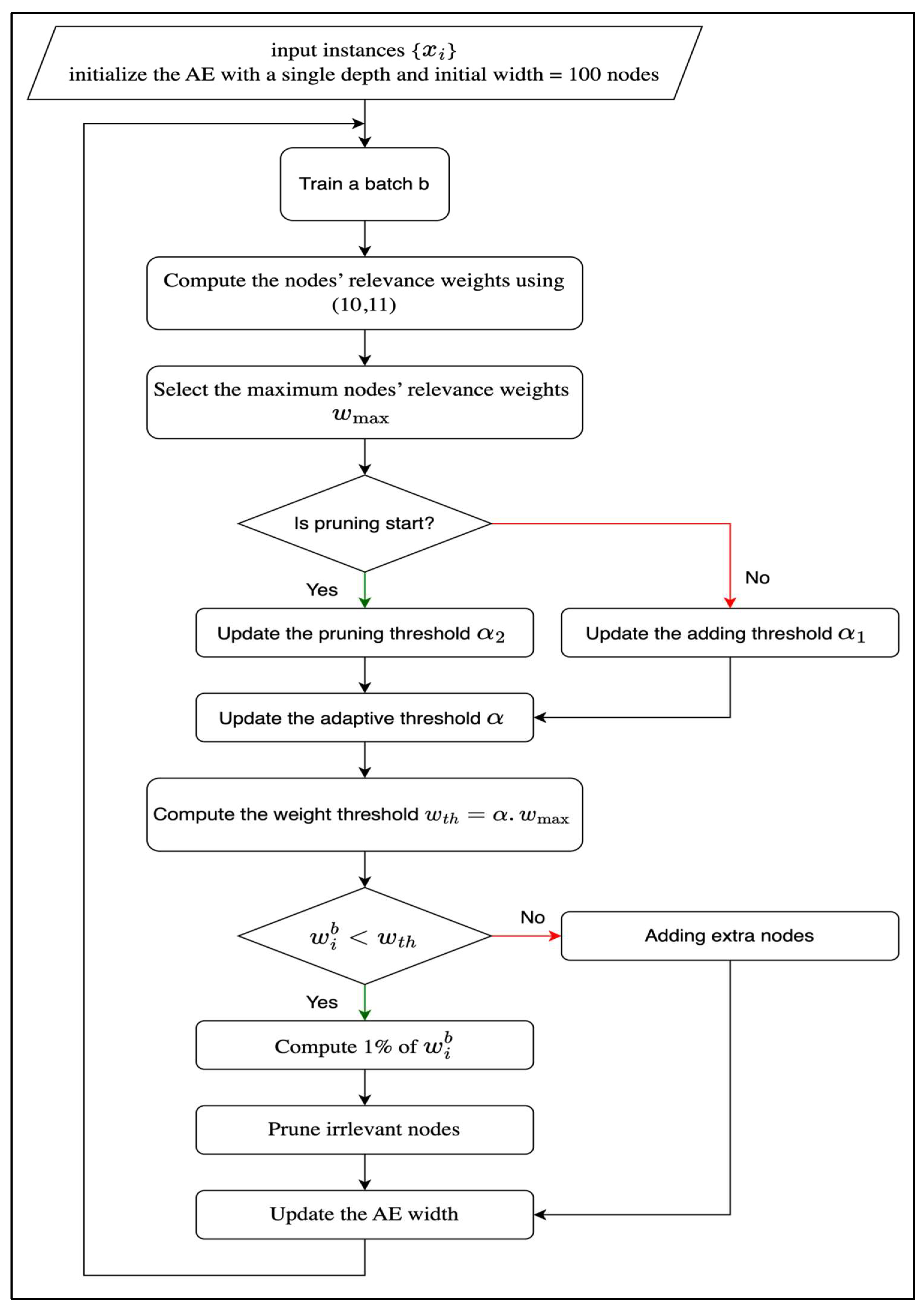
During the training phase, the encoder’s width was initially set to 100 nodes. It was incrementally increased by 10 nodes per batch until the first pruning occurred. The initial number of 100 hidden nodes and the incremental addition of 10 nodes per batch were selected as practical and computationally efficient defaults, consistent with common practice in adaptive architecture methods. These values allow the network to grow gradually while maintaining manageable training times. Importantly, due to the built-in relevance-weighting and pruning mechanisms, the final architecture is not highly sensitive to these choices. The model adaptively converges to a suitable width regardless of the initial or incremental size. Thus, these settings primarily affect convergence speed rather than the final performance. Following this, pruning was progressively applied until the model converged and the optimal width was achieved. The autoencoder (AE) hyperparameters, including learning rate, batch size, optimizer, and loss function, were configured as detailed in

Table 2. Configuration of hyperparameters.

Hyperparameter	MNIST	CIFAR-10	Parkinson	Epilepsy
Optimizer	Adam	Adam	Adam	Adam
Loss function	Binary Cross-Entropy	Binary Cross-Entropy	Mean Squared Error	Mean Squared Error
Learning rate	0.001	0.0001	0.0001	0.001
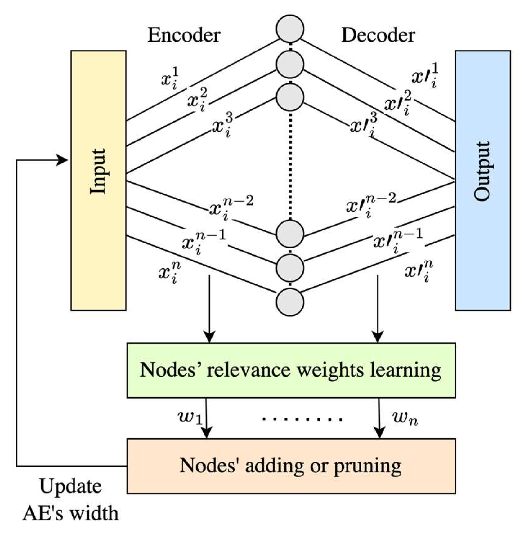
Batch size	256	64	64	128

. To evaluate the performance of the AE, features were extracted from the encoder and subsequently classified using two classifiers: a Support Vector Machine (SVM) and a SoftMax layer. While the training of the WAAE is entirely unsupervised, we use a SoftMax classifier only for post-hoc evaluation purposes. Specifically, once the autoencoder has learned the latent representations, a separate SoftMax layer is trained using the encoded features to assess their discriminative power. This approach does not influence the learning of the autoencoder itself. Furthermore, the structure of the latent space can also be evaluated without labels using metrics such as clustering quality, but labeled data is used here solely to quantify classification accuracy as a means of comparison with other models.

4.2.1. Performance Evaluation of the Proposed Approach on Benchmark Datasets

The proposed WAAE is trained using two benchmark datasets, MNIST [36] and CIFAR-10 [37], to assess its ability to dynamically learn the width of an AE in an unsupervised manner.

• Learned width dynamics

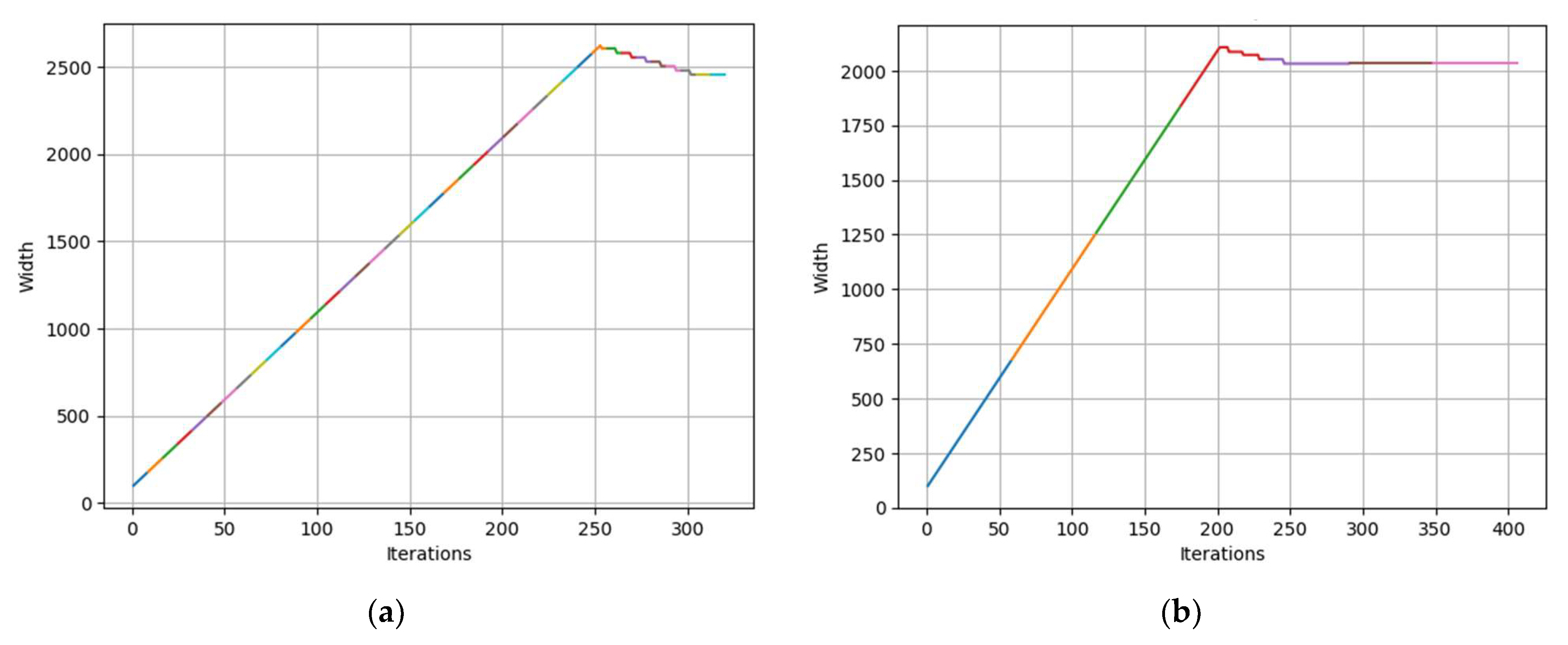
Figure 6 illustrates the evolution of the number of active nodes (i.e., the learned width) across training iterations for both the MNIST [36] and CIFAR-10 [37] datasets. In the early iterations, the number of nodes increases rapidly, reflecting the model’s adaptive expansion to capture complex patterns in the input data. For MNIST, the node count peaks at around iteration 250, whereas for CIFAR-10, the maximum is reached near iteration 300. Beyond these peaks, the model begins pruning less informative or redundant nodes, thereby reducing the architecture’s size. This pruning behavior helps prevent saturation and encourages model efficiency. Ultimately, the number of nodes stabilizes, converging to 1593 for MNIST and 1896 for CIFAR-10. These final widths reflect the respective complexities of the datasets and confirm the model’s ability to dynamically adapt its architecture.

• Convergence analysis

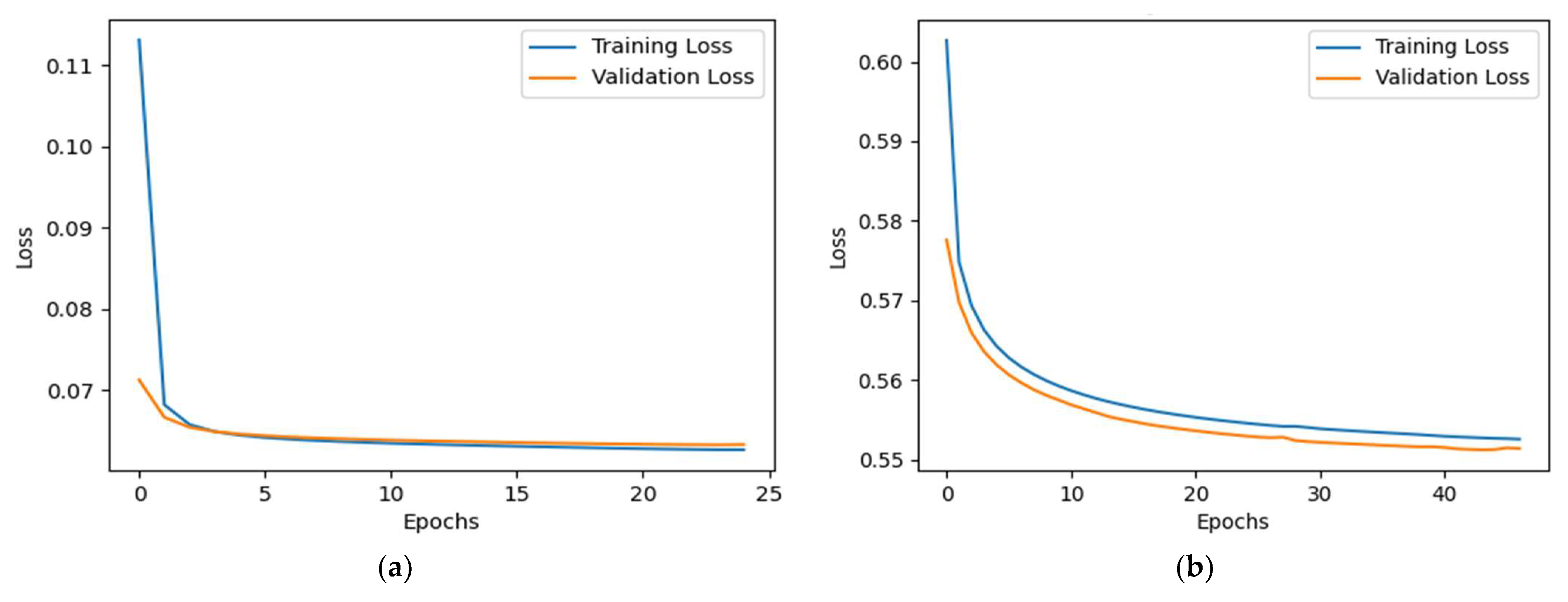
Figure 7 shows the training and validation loss curves over epochs. For MNIST, both losses decrease rapidly and converge closely within the first few epochs, with minimal discrepancy between the curves, indicating efficient learning and low overfitting. In contrast, CIFAR-10 shows a slower, steady decline in both losses, consistent with the dataset’s greater complexity. Notably, the validation loss remains slightly below the training loss throughout training on CIFAR-10, suggesting that the model generalizes well. Overall, both datasets demonstrate smooth and stable convergence, with MNIST exhibiting faster learning dynamics and CIFAR-10 requiring more training epochs to achieve similar performance stability.

• Performance metrics

Table 3. Final learned widths and classification accuracies for both the MNIST and CIFAR-10 datasets.

Dataset	MNIST		CIFAR-10
Learned Width	1593		1896
Classifier	SoftMax	SVM	SoftMax	SVM
Accuracy	95.97%	96.79%	44.66%	41.13%

presents the final learned widths and classification accuracies for both the MNIST and CIFAR-10 datasets using two classifiers: SoftMax and SVM. The learned width of the encoder stabilizes at 1593 nodes for MNIST and 1896 for CIFAR-10, indicating that the model adapts to the complexity of each dataset by allocating more representational capacity for the more challenging CIFAR-10. In terms of classification performance, both classifiers achieve high accuracies on MNIST, with SVM slightly outperforming SoftMax (96.79% vs. 95.97%), suggesting that the extracted features are highly discriminative for this relatively simple digit recognition task. However, for CIFAR-10, the accuracies are considerably lower, 44.66% with SoftMax and 41.13% with SVM, reflecting the increased difficulty of the dataset.

• Comparative evaluation with manual tuning

Table 4. Comparison between the manual tuning and dynamic learning approaches in terms of learned parameters, training time, and testing time for both MNIST and CIFAR-10 datasets.

Dataset	MNIST		CIFAR-10
Learning Type	Manual	Dynamic	Manual	Dynamic
Learned parameter	201,499,534	2,500,201	1,112,801,032	11,653,992
Train time (s)	48,963.16	701.06	874,853.23	413.14
Test time (s)	186.11	0.55	1025.81	0.70

highlights the contrast between the manual tuning and dynamic learning approaches in terms of learned parameters, training time, and testing time for both MNIST and CIFAR-10 datasets. The dynamic approach demonstrates a significant reduction in computational complexity and resource usage while maintaining effective model training. For the MNIST dataset, manual tuning results in over 201 million parameters, whereas the dynamic method learns only around 2.5 million parameters. It exhibits a reduction by nearly 99%. Similarly, for CIFAR-10, the parameter’s count drops from over 1.1 billion to approximately 11.6 million, reflecting a similar magnitude of improvement. This reduction in model size translates directly into drastic savings in training and testing time. Training time is reduced from roughly 48,963 s to 701 s for MNIST and from 874,853 s to just 413 s for CIFAR-10. Testing time also benefits from this efficiency, decreasing from 186.11 s to 0.55 s on MNIST, and from 1025.81 s to 0.70 s on CIFAR-10. These improvements underscore the effectiveness of the dynamic approach in achieving high computational efficiency and scalability, particularly important when dealing with large-scale data or resource-constrained environments. Thus, the proposed dynamic learning approach not only significantly reduces model complexity and runtime but also maintains competitive accuracy, making it a highly attractive alternative to traditional manual tuning methods.

In fact, the dynamic approach provides substantial advantages over manual tuning when determining a model’s width. Specifically, manual addition necessitates an exhaustive search process to determine the optimal width, which requires significant time and computational resources. This is because the model must be retrained with various widths. Furthermore, the features’ efficacy frequently depends upon the dataset, rendering manual methods less efficient and adaptable. In contrast, dynamic strategies enable the model to derive the optimal width from the data by self-adjusting its architecture during training. This adaptive process guarantees the model captures significant patterns without saturation or underfitting.

4.2.2. Performance Evaluation of the Proposed Approach on Real Datasets

The performance of the proposed approach in dynamically learning the width of AE is assessed using two real datasets: Parkinson’s [38] and Epilepsy [39]. Since the two datasets are unbalanced, the F1 measure is used to assess the model’s performance.

• Learned width dynamics

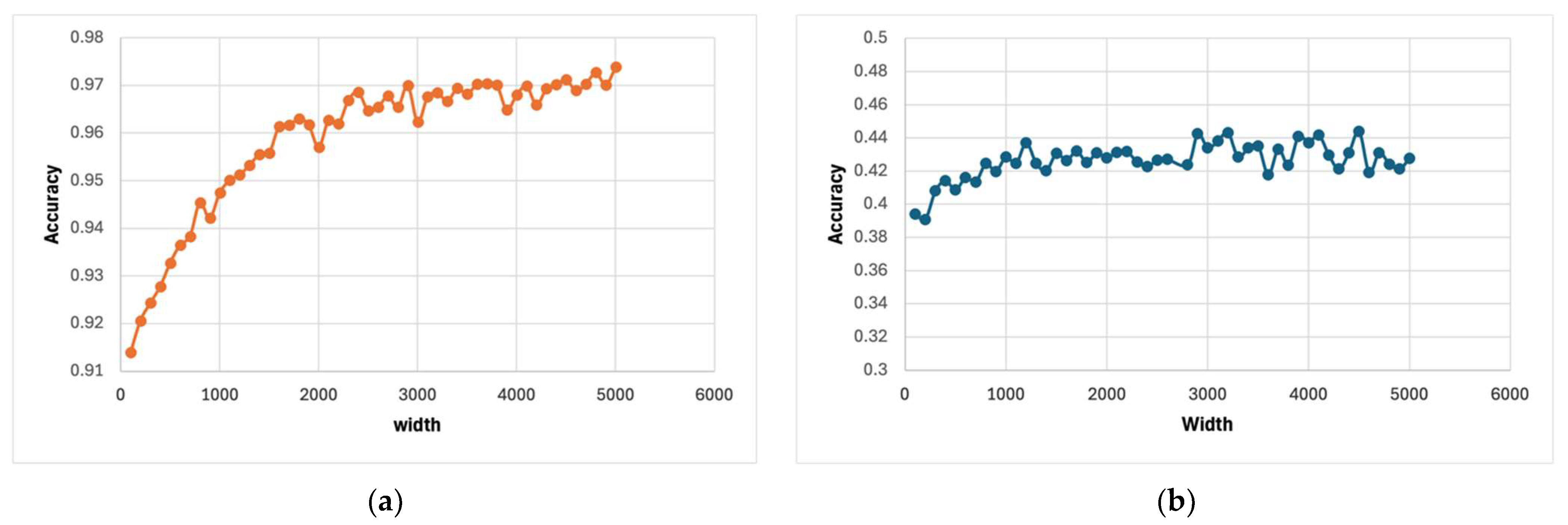
Figure 8 shows the learned width for the two real datasets. As can be seen, the number of nodes for Parkinson’s reaches its maximum at iteration 250, when the model converges to 2454 nodes. On the other hand, the Epilepsy dataset reaches its maximum at iteration 200 and converges to 2032 nodes.

• Convergence analysis

Similarly, Figure 9 shows the training and validation loss for the two datasets. For the Parkinson’s dataset, which contains only 756 instances, the validation loss converges to a lower value (~0.6) than the training loss (~0.8). This unusual pattern may suggest that the model generalizes better on the validation set.

• Performance metrics

Table 5. Final learned widths, classification accuracies, and F1-score for both the Parkinson and Epilepsy datasets.

Dataset	Parkinson		Epilepsy
Learned Width	2454		2032
Classifier	SoftMax	SVM	SoftMax	SVM
Accuracy	87.04%	90.13%	65.32%	68.65%
F1_Score	86.45%	89.89%	65.21%	68.69%

reports the learned widths with respect to the two datasets. For the Parkinson dataset, the width is 2454, indicating a relatively high-dimensional feature space. This suggests that the dataset may contain a significant amount of detailed or complex information, potentially offering more nuanced patterns for the classifiers to capture. In contrast, the Epilepsy dataset has a width of 2032, which is slightly lower, suggesting fewer features or possibly a less complex data structure compared to the Parkinson dataset. Despite having fewer features, the Epilepsy dataset presents a greater challenge to both classifiers, as seen in the relatively lower accuracy and F1-scores.

• Comparative evaluation with manual tuning

The results in

Table 6. Comparison between the manual tuning and dynamic learning approaches in terms of learned parameters, training time, and testing time for the two real datasets.

Dataset	Parkinson		Epilepsy
Learning Type	Manual	Dynamic	Manual	Dynamic
Learned parameter	457,948,938	3,703,840	74,522,760	725,602
Train time (s)	10866.75	175.01	6192.44	176.62
Test time (s)	32.51	0.11	54.44	0.38

show the comparison between manual tuning and dynamic learning approaches, particularly highlighting the impact of different model widths. In the manual tuning approach, the model’s width is varied, and experiments are repeated with different widths to identify the optimal configuration for the dataset. For the Parkinson dataset, the manual approach leads to a substantial number of learned parameters (457,948,938), as the width is likely set to large values in an attempt to capture more complex patterns. Similarly, for the Epilepsy dataset, manual tuning results in 74,522,760 learned parameters. This approach requires significant experimentation with different widths, resulting in longer training times, 10,866.75 s for Parkinson and 6192.44 s for Epilepsy. These extended times reflect the repeated trials to find the best width configuration. On the other hand, the dynamic learning approach, which doesn’t involve manual width adjustments but adapts automatically to the data, uses far fewer parameters (3,703,840 for Parkinson and 725,602 for Epilepsy), leading to a much more efficient model. As a result, dynamic learning drastically reduces both training time, 175.01 s for Parkinson and 176.62 s for Epilepsy, and testing time (0.11 s for Parkinson and 0.38 s for Epilepsy). Therefore, while manual tuning requires experimentation with different widths to find the optimal configuration, dynamic learning provides a more efficient alternative by automatically determining the best parameters, resulting in faster training and testing times while reducing model complexity.

4.2.3. Performance Comparison of the Proposed Approach with State-of-the-Art Models on Benchmark Datasets

In this experiment, the performance of the proposed method is evaluated against several state-of-the-art approaches specifically designed to adaptively determine the optimal width of autoencoders (AEs). The three most relevant and advanced methods considered for comparison are DEVDAN [18], SAQN [21], and NDL [17]. Moreover, two configurations for the SAQN model are considered with and without epochs since the original version considers only one epoch. As previously discussed, DEVDAN (Deep Evolving Denoising Autoencoder Network) is a self-adaptive model that dynamically adjusts the width of its AE by adding or pruning neurons based on the Network Significance (NS) metric. The NS value is computed using the bias and variance of the encoder–decoder model. Before updating network parameters through a combination of generative and discriminative training, a SoftMax layer is appended to facilitate discriminative testing. This process follows a prequential “test-then-train” approach. Similarly, SAQN (Self-Adaptive Quasi-Autoencoder Network) adopts the same structural framework as DEVDAN but updates its network parameters using generative training exclusively. Neurons are added or removed based on the estimated NS value, allowing the model to adaptively reshape its architecture without engaging in discriminative learning phases. In contrast, NDL (Neurogenesis Deep Learning) is a dynamic deep learning approach that adds neurons only when the model fails to adequately reconstruct the input, as indicated by reconstruction error. While effective, NDL is memory-intensive due to its reliance on storing past samples for retraining and its progressively expanding architecture. Moreover, it requires frequent retraining and multiple forward passes to stabilize the updated network, making it computationally expensive. To assess the effectiveness of the proposed approach, experiments are conducted on the MNIST [36] and CIFAR-10 [37] benchmark datasets. A SoftMax classifier is used in all cases to evaluate classification performance after the final AE model is learned. DEVDAN [18], SAQN [21], and SAQN with epochs adopt the MSE loss function as specified by their approaches, while NDL [17] and Width-Adaptive AE adopt Binary Cross-Entropy.

• Learned width dynamics and performance metrics for MNIST

Table 7. Performance measure comparison on the MNIST dataset.

Model	Accuracy	Train Loss	Test Loss	Learned Width
DEVDAN	90.60%	0.2211	0.2186	14
SAQN	86.37%	0.1378	0.1433	258
SAQN with epochs	89.61%	0.1034	0.1015	258
NDL	95.03%	0.12	0.1208	560
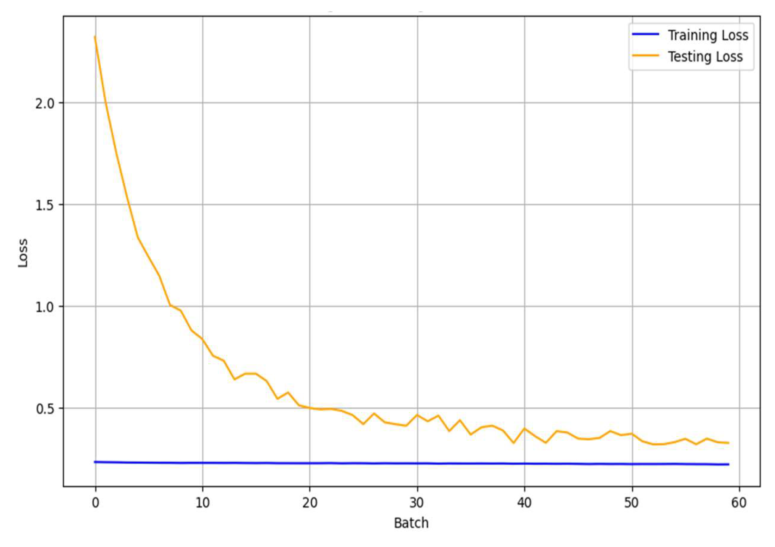
WAAE	95.97%	0.0627	0.0629	1593

presents a comprehensive comparison of performance metrics across several models on the MNIST dataset. The proposed WAAE achieves the highest accuracy at 95.97%, outperforming all baselines, including NDL (95.03%), DEVDAN (90.60%), SAQN with epochs (89.61%), and standard SAQN (86.37%). In terms of training and testing loss, the WAAE also records the lowest values (0.0627 and 0.0629, respectively), indicating effective optimization. This contrasts with the higher loss values observed in DEVDAN and SAQN, which correlates with their lower classification performance. A key distinction lies in the learned network width: the WAAE dynamically expands to 1593 neurons, significantly wider than NDL (560), SAQN (258), and DEVDAN (14). This flexibility enables the proposed model to better capture the underlying complexity of the data, contributing to its superior accuracy and lower loss. These results highlight the effectiveness of the WAAE. The superior performance of the WAAE can be attributed not only to its ability to dynamically learn an optimal network width but also to its robustness against the limitations inherent in competing models. For instance, while NDL achieves high accuracy, its architecture heavily depends on user-defined parameters such as the reconstruction threshold and MaxOutlier. These parameters require manual tuning through a trial-and-error process, as there is no standardized approach for their selection. As a result, NDL’s performance is sensitive to configuration choices, which can lead to inconsistent convergence and suboptimal generalization if not thoroughly optimized. The model’s behavior demonstrates that varying the MaxOutlier percentage affects node expansion in unintuitive ways, further complicating its tuning. In contrast, the WAAE eliminates this dependency by autonomously adjusting its width based on learning dynamics, achieving better convergence as evidenced by its significantly lower training and testing losses. Additionally, models like DEVDAN and SAQN suffer from structural limitations. DEVDAN’s use of only 14 neurons leads to high reconstruction errors and poor generalization due to its constrained representational capacity. This is confirmed by the DEVDAN model’s training loss displayed in Figure 10. It is nearly constant, with minimal changes observed across batches. This implies that the model may not be learning effectively. Although SAQN utilizes more neurons, its static allocation (258 nodes) and lack of dynamic width adaptation result in inefficiencies, as reflected by its relatively high test loss. Moreover, as shown in Table 7, by increasing the number of epochs, the SAQN model exhibits minimal improvements in both train and test losses with a little change in accuracy. There is no improvement to the model’s width, which implies that it has reached its learning capacity. This may be the result of over-regularization or restricted node adaption. The WAAE, by contrast, adaptively scales its architecture to 1593 neurons, enabling it to learn complex feature representations more effectively. This dynamic capacity, free from manual hyperparameter constraints and structural rigidity, allows it to consistently outperform the baseline models in both accuracy and reconstruction loss.

• Computational complexity and time for MNIST

Table 8. Computational complexity and time comparison of Width-Adaptive AE and state-of-the-art approaches on the MNIST dataset.

Model	Train Time (s)	Test Time (s)	Training FLOPs (G)	Testing FLOPs (G)	Model’s FLOPs (G)
DEVDAN	628.4579	0.1964	20.5383	0.48424	0.00007
SAQN	132.4657	1.8377	116.6587	8	0.0008
SAQN with epochs	417.1866	0.5107	466.32379	8	0.0008
NDL	497.8599	0.8997	34162.173	17.562	0.00198
WAAE	701.0619	0.5542	2789.455	49.9	0.00499

presents a comparative analysis of the computational complexity and processing time of the WAAE against several state-of-the-art models on the MNIST dataset. While the WAAE exhibits the longest training time (701.06 s), it achieves a competitive testing time (0.5542 s), outperforming models like NDL (0.8997 s) and SAQN (1.8377 s). Although DEVDAN remains the fastest in testing (0.1964 s), its limited architecture restricts performance. In terms of training GFLOPs, the WAAE requires 2789.45 GFLOPs, significantly less than NDL’s computationally intensive 34,162.17 GFLOPs, yet much higher than the lightweight DEVDAN and SAQN models. The testing GFLOPs of the WAAE (49.9) reflect its richer representational capacity, which supports its superior performance. Furthermore, the model’s total FLOPs (0.00499 GFLOPs) are the highest among the compared approaches, consistent with its broader network width and adaptive design. In contrast, models like DEVDAN and SAQN demonstrate minimal computational requirements but suffer from limited learning capabilities and lower accuracy. Despite its higher computational demand, the WAAE offers a more favorable trade-off between accuracy and complexity, demonstrating that its dynamic architecture and resource allocation lead to improved learning and generalization, justifying the increased training cost.

The results in Table 8 further reinforce the effectiveness of the WAAE by contextualizing its computational cost in light of architectural and operational efficiencies. Unlike NDL, which adopts a class-by-class training strategy requiring repeated replay and adjustment after each new class, the WAAE is trained on all classes simultaneously. This enables it to generalize more effectively without excessive reliance on replay mechanisms that inflate FLOPs. In fact, NDL reaches over 34,000 training GFLOPs due to continual reprocessing of prior data. Furthermore, NDL’s sequential learning approach risks overfitting to early classes, undermining its generalization. Similarly, while DEVDAN is lightweight with only 14 nodes and incurs just 21 GFLOPs during training, its three-step batch processing framework adds overhead and limits convergence. DEVDAN struggles to stabilize, continuously pruning and adding nodes even in later training batches, which hinders consistent learning. In contrast, the WAAE achieves stable convergence within a few epochs by dynamically adjusting its width in response to learned patterns, resulting in superior reconstruction performance and the highest accuracy (95.97%) among all models. SAQN, despite requiring up to 467 GFLOPs during training, fails to achieve similar performance due to inadequate iterative learning and a static architecture that underutilizes its computational potential. The model’s inability to dynamically expand to meet data complexity results in poor feature extraction and elevated reconstruction loss. This results in inferior reconstructions, as demonstrated by the sample instances from the MNIST dataset in Figure 11. Notably, the WAAE also excels in inference efficiency. It delivers a faster test time (0.5542 s) than both SAQN and NDL, despite utilizing significantly more nodes (1593). This suggests that the model’s architecture is not only scalable but also optimized for real-time deployment. Thus, although the WAAE entails higher training cost, its design allows it to balance complexity and performance more effectively than its peers, justifying the resource investment with its superior learning capacity and generalization.

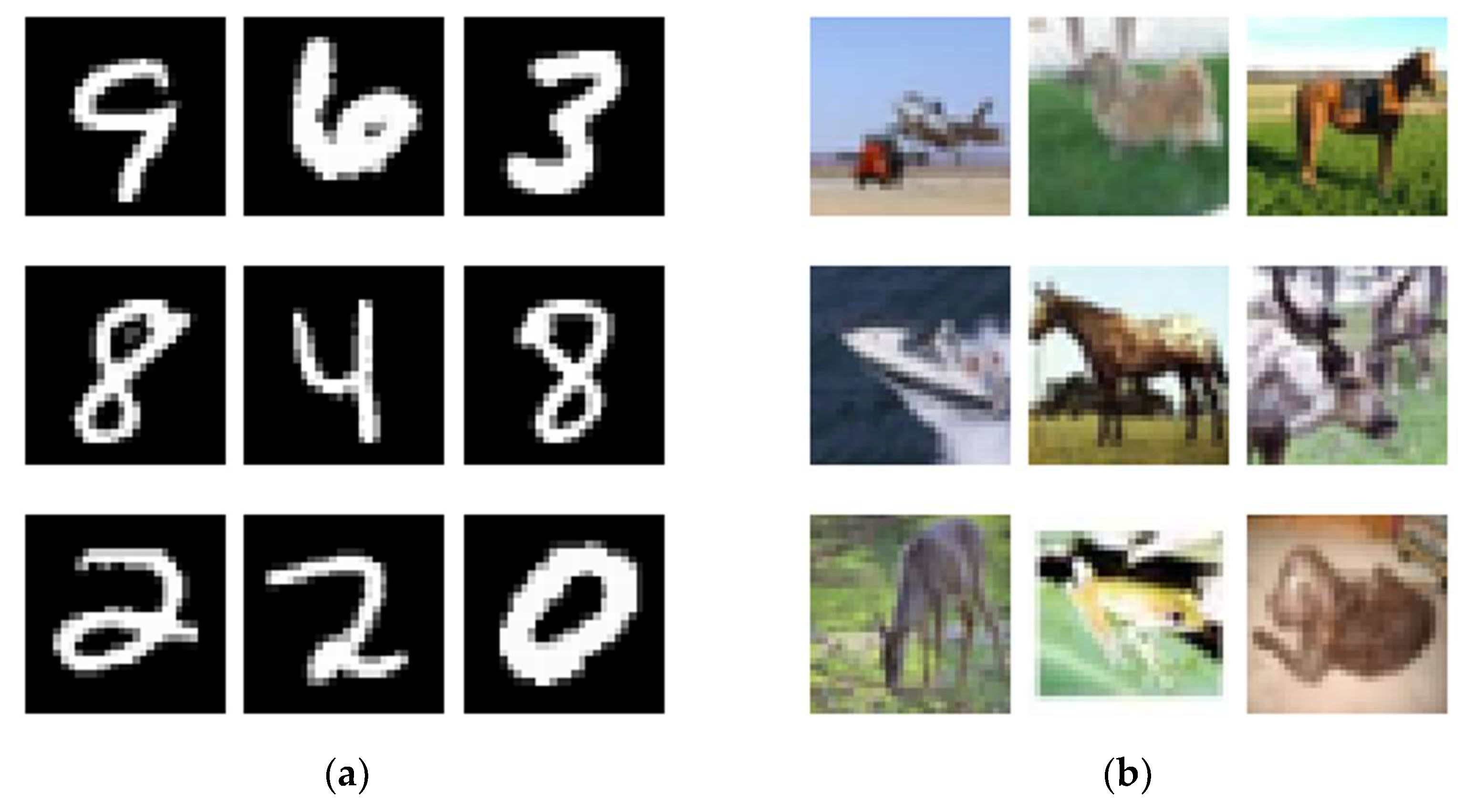
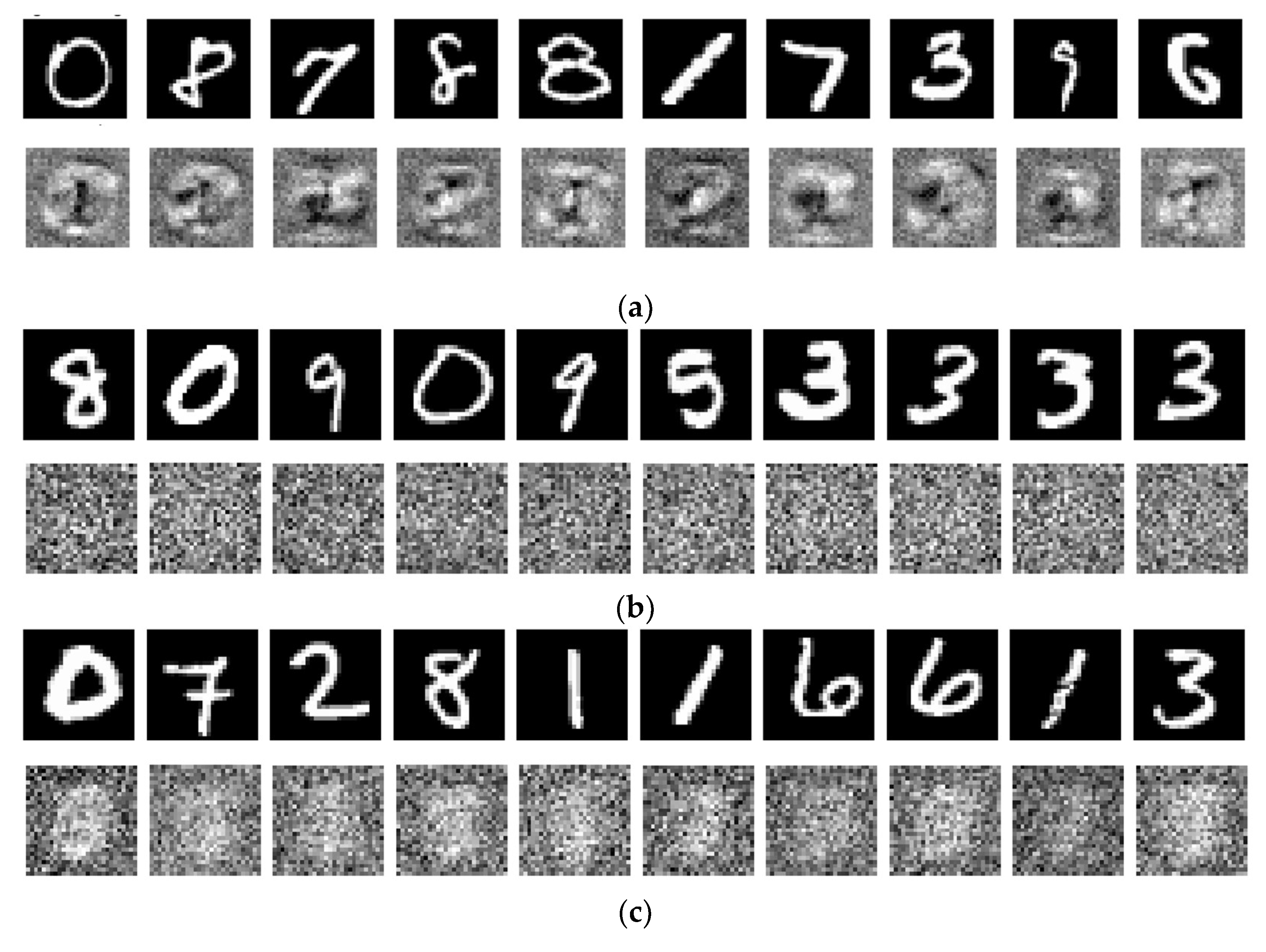
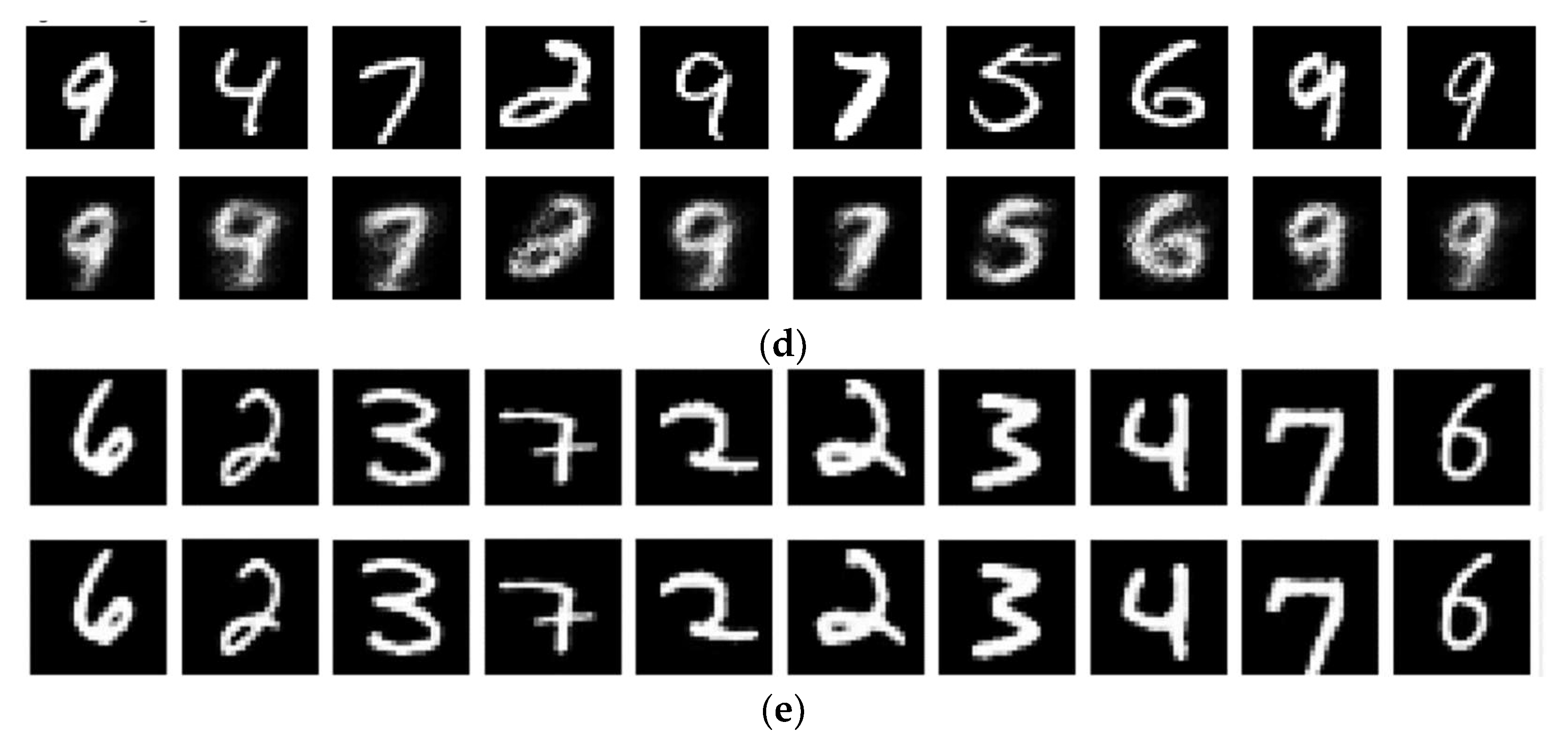
Figure 11 provides a visual comparison of the reconstruction quality of 10 random MNIST digit instances using five different models: DEVDAN, SAQN, SAQN without epochs, NDL, and WAAE. The top row in each subfigure shows the original digit images, while the bottom row displays the corresponding reconstructions. Among the models, WAAE clearly produces the most accurate and visually faithful reconstructions, with digits that are crisp, well-formed, and closely match the original inputs in both shape and structure. The NDL model also performs well, producing generally recognizable digits with minor blurring, indicating a solid capacity to capture data representations. In contrast, the DEVDAN model yields reconstructions that are blurred and less distinct, though some digit structures remain identifiable. Both SAQN and SAQN without epochs perform poorly, with reconstructions that resemble random noise rather than digit shapes, reflecting a failure to learn meaningful latent representations. These visual results align with earlier quantitative findings and underscore the effectiveness of WAAE’s adaptive architecture and appropriate loss function in achieving superior reconstruction and representational quality.

• Learned width dynamics and performance metrics for CIFAR-10

Table 9. Performance measure comparison on CIFAR-10 dataset.

Model	Accuracy	Train Loss	Test Loss	Width
DEVDAN	41%	0.5660	0.5583	262
SAQN	33.89%	0.2428	0.2560	257
SAQN with epochs	32.99%	0.0604	0.0623	257
NDL	37.47%	0.6468	0.6469	798
WAAE	44.66%	0.5526	0.5538	1896

presents a performance comparison of several models on the CIFAR-10 dataset using various evaluation metrics, including accuracy, train and test loss, and model width. Among the models, the WAAE achieves the highest accuracy at 44.66%, which can be attributed to its large width (1896). DEVDAN also shows reasonable performance with 41% accuracy and balanced train and test losses, indicating good generalization despite its relatively small width of 262. In contrast, the SAQN models, both with and without epoch-based training, report the lowest accuracies (33.89% and 32.99%, respectively) even though they achieve very low loss values. This suggests a misalignment between the MSE loss function used and the classification nature of the task, leading to poor predictive performance. The NDL model, with a wider architecture (width of 798) achieves moderate accuracy (37.47%) but does not outperform DEVDAN, underscoring that higher width alone does not guarantee better performance.

The superior performance of the WAAE in Table 9 can be further understood in light of how model width is determined in comparison to other models such as NDL. Notably, NDL relies on user-defined thresholds. Specifically, the MaxOutlier percentage is used to determine its width. This approach introduces variability and a degree of uncertainty into the model configuration, as the width is highly sensitive to this parameter. For example, when the MaxOutlier threshold is decreased to 10% of the data, the NDL model reaches its maximum width, with a corresponding loss of 0.63. Conversely, increasing the threshold to 30% reduces the width significantly to 308, yet the loss remains nearly unchanged. This demonstrates that the NDL model’s performance does not scale linearly with its width, and that finding an optimal configuration requires trial and error that may not generalize well across datasets.

In contrast, the WAAE employs a more systematic and data-driven method for determining width, enabling it to dynamically adjust its architecture in response to the data characteristics without requiring manual threshold tuning. This adaptability likely contributes to its ability to achieve the highest accuracy (44.66%) among all models in the comparison. The model’s large width of 1896 further enhances its capacity to learn complex patterns in the CIFAR-10 dataset. The consistency between its low train and test losses (0.5526 and 0.5538, respectively) also reflects strong generalization. Therefore, the WAAE demonstrates the advantages of automated architecture tuning and the use of suitable loss functions, which together result in more reliable and higher classification performance than models like NDL that depend on manually selected, dataset-specific parameters.

• Computational complexity and time for CIFAR-10

Table 10. Computational complexity and runtime comparison of Width-Adaptive AE and state-of-the-art approaches on the CIFAR-10 dataset.

Model	Train Time (s)	Test Time (s)	Training FLOPs (G)	Testing FLOPs (G)	Model’s FLOPs (G)
DEVDAN	471.3421	0.6918	877.0574	32.3301	0.00483
SAQN	198.0413	0.6849	379.3614	31.6	0.00316
SAQN with epochs	1258.4149	0.4738	3034.2842	31.6	0.00316
NDL	965.3241	2.9983	131,579.845	99.287	0.00490
WAAE	413.1391	0.698	8246.7779	233.0302	0.0233

presents a comparison of computational complexity and runtime performance for several models on the CIFAR-10 dataset, highlighting the trade-offs between training cost, inference efficiency, and model complexity. The WAAE, while more computationally intensive than some alternatives, demonstrates a balanced trade-off between performance and resource usage. It achieves a training time of 413.14 s, which is significantly faster than models like NDL (965.32 s) and SAQN with epochs (1258.41 s), despite having higher training FLOPs at 8246.78 gigaflops. This suggests that the WAAE is computationally heavier but more optimized. At test time, it maintains a competitive speed (0.698 s), similar to DEVDAN (0.6918 s) and SAQN (0.6849 s), although it incurs the highest testing FLOPs at 233.03 gigaflops, reflecting its increased model complexity. The model’s FLOPs per inference (0.0233 G) are also the highest among all compared approaches, corresponding to its larger width and adaptive architecture. In contrast, models like SAQN and DEVDAN are computationally lighter but offer lower accuracy, while NDL exhibits extremely high training FLOPs (131,579.84 G) without delivering superior predictive performance. Consequently, the WAAE achieves the best balance between training efficiency, inference speed, and classification accuracy, making it a robust choice when moderate computational resources are available.

It is important to note that the compared models, DEVDAN [18], SAQN [21], and NDL [17], employ simpler node selection or importance heuristics such as activation frequency and threshold-based pruning. These models therefore serve as effective baselines to isolate the impact of the inner-product-based relevance weighting used in our approach. The consistently superior performance of the WAAE across both accuracy and computational cost demonstrates the effectiveness of our more principled node relevance strategy.

4.2.4. Performance Comparison of the Proposed Approach with State-of-the-Art Models on Real Datasets

A comprehensive performance comparison was performed between the proposed WAAE and several state-of-the-art models across the two considered real-world datasets. The evaluation focuses on key performance metrics such as accuracy, F1-score, loss values, computational complexity, and model width.

• Learned width dynamics and performance metrics for Parkinson’s

Table 11. Performance measure comparison on Parkinson’s dataset.

Model	Accuracy	F1-Score	Train Loss	Test Loss	Width
DEVDAN	81.58%	81%	1.2428	1.1740	104
SAQN	76.31%	77.86%	1.1120	1.0776	256
SAQN with epochs	68.42%	70.88%	1.0123	1.0717	256
NDL	50.66%	53.62%	1.0328	1.0169	200
WAAE	87.04%	86.45%	0.7551	0.6925	2454

presents a performance comparison of several models on the Parkinson’s dataset, evaluating key metrics such as accuracy, F1-score, training loss, testing loss, and model width. Among all models, the WAAE demonstrates the strongest performance across all metrics, achieving the highest accuracy (87.04%) and F1-score (86.45%), along with the lowest training (0.7551) and testing loss (0.6925). This indicates that the model is not only highly accurate but also generalizes well, maintaining low error rates across both seen and unseen data.

In contrast, while DEVDAN shows moderate results with an accuracy of 81.58% and F1-score of 81%, it still falls short of the WAAE. Its training and test losses are considerably higher (1.2428 and 1.1740), suggesting less efficient learning and potential overfitting or underfitting. SAQN, although having a wider architecture (width = 256), delivers slightly lower performance (76.31% accuracy, 77.86% F1-score), with marginally better losses compared to DEVDAN. Interestingly, SAQN with epochs performs even worse, indicating that simply increasing training epochs does not lead to better performance, possibly due to overfitting or a misaligned training strategy.

The NDL model performs the worst across the board, with only 50.66% accuracy and 53.62% F1-score, despite having a wider architecture than DEVDAN. Its relatively low training and test losses do not translate into meaningful classification performance, suggesting that the model may struggle with learning discriminative features for this dataset.

The WAAE’s high width (2454), paired with low loss values and superior classification metrics, demonstrates the advantage of its dynamic architecture. By adaptively adjusting model width to the complexity of the data, it successfully captures informative representations, outperforming static-width models that rely on trial-and-error or fixed parameters. This reinforces the importance of architectural flexibility and data-driven design in achieving optimal performance on medical datasets like Parkinson’s.

• Computational complexity and time for Parkinson’s

Table 12. Computational complexity and runtime comparison of Width-Adaptive AE and state-of-the-art approaches on Parkinson’s dataset.

Model	Train Time	Test Time	Training FLOPs (G)	Testing FLOPs (G)	Model’s FLOPs (G)
DEVDAN	10.8530	0.3858	1.0896	0.04792	0.00016
SAQN	80.2866	0.1774	1.12255	0.11704	0.00077
SAQN with epochs	79.7202	0.1691	1.71629	0.11704	0.00077
NDL	2.3384	0.007	1.321611	0.091686	0.00030
WAAE	175.0063	0.109	281.31	1.1248	0.00740

highlights the computational complexity and runtime performance of the models on the Parkinson’s dataset, emphasizing the trade-offs associated with the WAAE. While the WAAE records the highest training time (175.01 s) and training FLOPs (281.31 G), it maintains a relatively efficient test time (0.109 s), outperforming DEVDAN and closely matching SAQN variants. Its higher testing FLOPs (1.1248 G) and model FLOPs (0.0074 G) are a direct result of its significantly larger width, as also shown in Table 11. This relationship underscores the fact that the model’s time and computational complexity scale with its width. However, this increase in complexity translates into substantial performance gains, confirming that the adaptive width mechanism enables the model to learn richer representations and achieve superior results on the Parkinson’s dataset.

• Learned width dynamics and performance metrics for Epilepsy

Table 13. Performance measure comparison on the Epilepsy dataset.

Model	Accuracy	F1-Score	Train Loss	Test Loss	Width
DEVDAN	25.48%	16%	0.8749	0.9535	1323
SAQN	26.52%	26.35%	1.0313	1.1628	257
SAQN with epochs	27.04%	26.80%	0.8729	0.937	254
NDL	31.04%	24.60%	1.0201	0.9543	226
WAAE	65.32%	65.21%	0.7044	0.7899	2032

presents a comparative performance analysis of different models on the Epilepsy dataset, clearly highlighting the effectiveness of the WAAE. Among all the models, WAAE achieves the highest accuracy (65.32%) and F1-score (65.21%), outperforming all competing approaches by a substantial margin. This demonstrates its strong classification ability, especially on complex and imbalanced datasets like Epilepsy. Furthermore, it achieves the lowest training and testing loss values (0.7044 and 0.7899, respectively), indicating better learning stability and generalization. In contrast, other models such as DEVDAN, SAQN, and NDL perform significantly worse, with accuracies ranging between 25–31% and notably lower F1-scores, suggesting they struggle to capture meaningful patterns in the data. Although the WAAE has the largest model width (2032), this increased capacity enables it to represent complex temporal patterns more effectively, reinforcing the idea that adaptive width contributes significantly to its superior performance.

• Computational complexity and time for Epilepsy

Table 14. Computational complexity and runtime comparison of Width-Adaptive AE and state-of-the-art approaches on the Epilepsy dataset.

Model	Train Time (s)	Test Time (s)	Training FLOPs (G)	Testing FLOPs (G)	Model’s FLOPs (G)
DEVDAN	157.4705	1.1351	837742.704	2.3305	0.00048
SAQN	109.3301	0.2624	4.00266	0.069	0.00018
SAQN with epochs	255.3176	0.2189	79.94883	0.069	0.00018
NDL	18.4793	0.0426	40.180039	0.370098	0.00008
WAAE	176.6206	0.3758	174.0157	3.335	0.00145

presents a comparative analysis of the computational complexity and runtime performance of the WAAE against several state-of-the-art models using the Epilepsy dataset. Although the WAAE exhibits the highest test FLOPs (3.335 G) and model FLOPs (0.00145 G), it maintains competitive training time (176.62 s) and moderate training FLOPs (174.02 G). In contrast, DEVDAN, while having the lowest model FLOPs (0.00048 G), shows an exceptionally high training FLOPs (837742.70 G), suggesting inefficiency. SAQN variants achieve low model and test FLOPs but vary significantly in training time depending on epochs. NDL stands out with the shortest training and testing time and the lowest model FLOPs, but at the cost of slightly higher test FLOPs than SAQN. Overall, the WAAE strikes a balance between adaptability and computational efficiency, offering a favorable trade-off for real-time epilepsy data processing.

• Comparative evaluation with existing state-of-the-art models

These results further highlight the advantage of using the proposed inner-product-based relevance weighting mechanism compared to the simpler heuristics used in DEVDAN, SAQN, and NDL. Although these baseline models incorporate basic node evaluation methods, they fall short in adapting to data complexity as efficiently as our approach. This provides indirect but strong evidence of the contribution and necessity of our more structured weighting criterion.

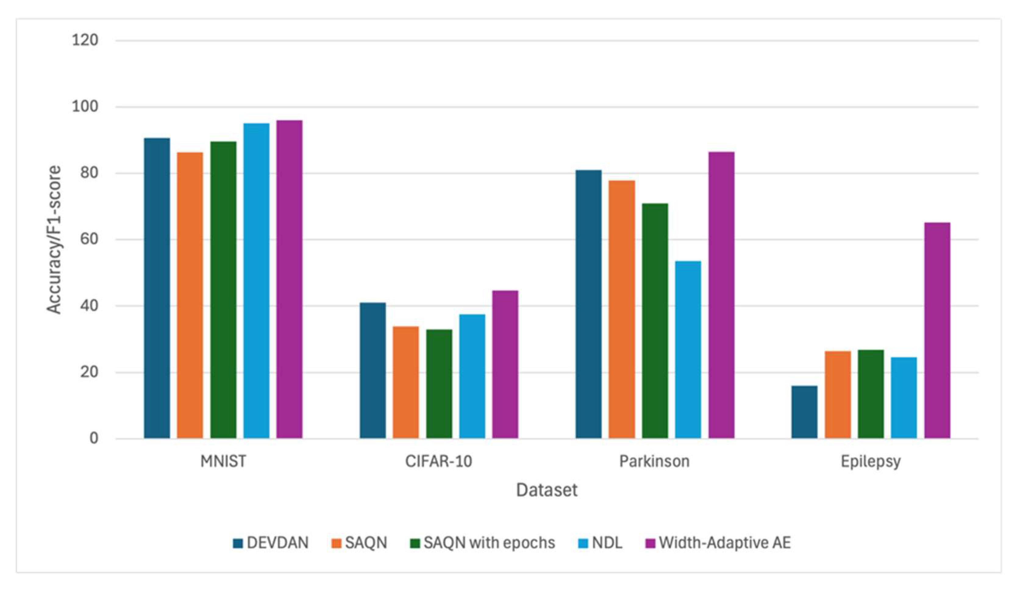
Figure 12 displays a bar chart comparing the accuracy or F1-score of five models, DEVDAN, SAQN, SAQN with epochs, NDL, and WAAE, across four datasets: MNIST, CIFAR-10, Parkinson, and Epilepsy. Since the real datasets are unbalanced, the F1-score is used for comparison rather than accuracy. WAAE consistently outperforms or matches other models in terms of accuracy or F1-score across all datasets. For MNIST, all models perform similarly with high accuracy (~90–100%), with WAAE slightly leading. In CIFAR-10, accuracies drop overall, but WAAE achieves the highest performance again. On the Parkinson dataset, WAAE shows a notable lead over others, achieving the highest F1-score among all models. Notably, on the challenging Epilepsy dataset, where other models hover around 20–30% F1-score, WAAE significantly outperforms them, achieving over 60%. This highlights its robustness and adaptability across varying data complexities and domains.

The experimental results across both benchmark (MNIST, CIFAR-10) and real-world (Parkinson, Epilepsy) datasets demonstrate that the proposed WAAE consistently achieves high classification accuracy while maintaining computational efficiency. The model dynamically adjusted its width by adding and pruning nodes, resulting in architectures that are both compact and effective. Compared to manually tuned and state-of-the-art models, the proposed method showed competitive or superior performance in terms of accuracy, training time, and resource utilization. These findings confirm the model’s ability to adapt to varying dataset complexities and support its effectiveness in both simple and challenging learning scenarios.

4.3. Discussion on Parameter Sensitivity

The exponent parameter $q$ in the cost function $J_{FC}\left(l\right)$ plays a critical role in shaping the distribution of relevance weights. Lower values of $q$ (closer to 1) result in more uniform relevance distributions, while higher values increase contrast, emphasizing nodes with better inner product preservation. This behavior aligns with principles from fuzzy entropy and attention mechanisms, where higher contrast sharpens selection but risks overfitting.

Similarly, the pruning threshold (used for removing low-relevance nodes) controls the trade-off between model compactness and expressiveness. A low threshold may retain redundant nodes, slowing convergence and increasing computational cost, while a high threshold could risk prematurely eliminating useful capacity. In practice, setting the threshold to a fraction of 70% of the maximum relevance weight ensures conservative yet effective pruning. Future work will include an empirical investigation of these parameter sensitivities to validate these theoretical insights and refine the default choices.

5. Conclusions

This paper introduced a novel Width-Adaptive Autoencoder (AE) that autonomously determines the optimal width of the network by learning node-level relevance weights. The proposed approach expands the network when necessary and prunes irrelevant nodes based on a dynamic optimization strategy. By integrating a new cost function, it enables simultaneous learning of architecture and parameters, leading to an efficient and adaptive model.

Experimental evaluations on both benchmark datasets (MNIST, CIFAR-10) and real-world datasets (Parkinson, Epilepsy) demonstrated the model’s ability to achieve competitive or superior accuracy with lower computational overhead compared to manually tuned or state-of-the-art approaches. These results highlight the method’s robustness, scalability, and practical applicability in diverse learning scenarios.

Despite its advantages, the current framework is limited to a single hidden layer. Future work will focus on extending the approach to multi-layer or hierarchical architectures, allowing for deeper and more expressive representations. Additionally, we aim to adapt the model for real-time and streaming data environments, where on-the-fly width adaptation can further enhance model efficiency. Exploring the joint optimization of both depth and width is also a promising direction that could lead to fully self-configuring deep learning architectures.

Moreover, while the proposed WAAE demonstrates promising results in terms of compression flexibility and reconstruction performance, several limitations should be acknowledged. First, although WAAE reduces model size during inference, its training process involves evaluating and optimizing multiple width configurations, which increases computational costs. This can become particularly demanding for large-scale or high-resolution datasets. Efficient approximation methods or layer-wise adaptation strategies could be explored to alleviate this burden. Moreover, the current method relies on empirically defined thresholds to guide width adaptation. These thresholds can significantly influence convergence behavior and model quality. A more principled or data-driven approach to adapt thresholds dynamically may improve robustness and reduce the need for manual tuning. In addition, the width adaptation mechanism is designed for offline training. Applying WAAE to streaming data or continual learning settings would require additional mechanisms to handle evolving data distributions and avoid catastrophic forgetting. Incorporating memory-efficient or incremental learning strategies could be a promising direction for extending WAAE’s applicability. Finally, while autoencoders are traditionally evaluated using reconstruction error, extending WAAE to downstream tasks such as classification, clustering, or anomaly detection requires further investigation. The effect of adaptive latent width on task-specific performance metrics remains an open question. Future work will aim to address these limitations by integrating adaptive threshold learning, accelerating training through surrogate optimization, and testing WAAE in online learning environments and diverse application domains.

References

1. Pedrycz, W.; Chen, S.-M. Deep Learning: Concepts and Architectures; Pedrycz, W., Chen, S.-M., Eds.; Springer International Publishing: Cham, Switzerland, 2020; Volume 866, ISBN 978-3-030-31755-3. [Google Scholar]
2. Alom, M.Z.; Taha, T.M.; Yakopcic, C.; Westberg, S.; Sidike, P.; Nasrin, M.S.; Hasan, M.; Van Essen, B.C.; Awwal, A.A.S.; Asari, V.K. A State-of-the-Art Survey on Deep Learning Theory and Architectures. Electronics 2019, 8, 292. [Google Scholar] [CrossRef]
3. Krizhevsky, A.; Sutskever, I.; Hinton, G.E. ImageNet Classification with Deep Convolutional Neural Networks. Commun. ACM 2017, 60, 84–90. [Google Scholar] [CrossRef]
4. Pang, G.; Shen, C.; Cao, L.; Hengel, A.V.D. Deep Learning for Anomaly Detection. ACM Comput. Surv. 2022, 54, 1–38. [Google Scholar] [CrossRef]
5. Srivastava, S.; Divekar, A.V.; Anilkumar, C.; Naik, I.; Kulkarni, V.; Pattabiraman, V. Comparative Analysis of Deep Learning Image Detection Algorithms. J. Big Data 2021, 8, 66. [Google Scholar] [CrossRef]
6. LeCun, Y.; Bengio, Y.; Hinton, G. Deep Learning. Nature 2015, 521, 436–444. [Google Scholar] [CrossRef]
7. Zhou, M.; Duan, N.; Liu, S.; Shum, H.-Y. Progress in Neural NLP: Modeling, Learning, and Reasoning. Engineering 2020, 6, 275–290. [Google Scholar] [CrossRef]
8. Chicco, D.; Sadowski, P.; Baldi, P. Deep Autoencoder Neural Networks for Gene Ontology Annotation Predictions. In Proceedings of the 5th ACM Conference on Bioinformatics, Computational Biology, and Health Informatics, New York, NY, USA, 20 September 2014; pp. 533–540. [Google Scholar]
9. Zhang, G.; Liu, Y.; Jin, X. A Survey of Autoencoder-Based Recommender Systems. Front. Comput. Sci. 2020, 14, 430–450. [Google Scholar] [CrossRef]
10. Hadi, F.; Yang, J.; Ullah, M.; Ahmad, I.; Farooque, G.; Xiao, L. DHCAE: Deep Hybrid Convolutional Autoencoder Approach for Robust Supervised Hyperspectral Unmixing. Remote Sens. 2022, 14, 4433. [Google Scholar] [CrossRef]
11. Alom, M.Z.; Taha, T.M. Network Intrusion Detection for Cyber Security Using Unsupervised Deep Learning Approaches. In Proceedings of the 2017 IEEE National Aerospace and Electronics Conference (NAECON), Dayton, OH, USA, 27–30 June 2017; pp. 63–69. [Google Scholar]
12. Devlin, J.; Chang, M.-W.; Lee, K.; Toutanova, K. BERT: Pre-Training of Deep Bidirectional Transformers for Language Understanding. arXiv 2018, arXiv:1810.04805. [Google Scholar]
13. OpenAI. Available online: https://openai.com/ (accessed on 5 February 2024).
14. Coates, A.; Ng, A.; Lee, H. An Analysis of Single-Layer Networks in Unsupervised Feature Learning. In Proceedings of the 14th International Conference on Artificial Intelligence and Statistics, Fort Lauderdale, FL, USA, 11–13 April 2011; Volume 15, pp. 215–223. [Google Scholar]
15. Alfayez, S.; Bchir, O.; Ben Ismail, M.M. Dynamic Depth Learning in Stacked AutoEncoders. Appl. Sci. 2023, 13, 10994. [Google Scholar] [CrossRef]
16. Cohoon, J.; Kairo, J.; Lienig, J. Evolutionary Algorithms for the Physical Design of VLSI Circuits. In Advances in Evolutionary Computing; Springer: Berlin/Heidelberg, Germany, 2003; pp. 683–711. [Google Scholar]
17. Draelos, T.J.; Miner, N.E.; Lamb, C.C.; Cox, J.A.; Vineyard, C.M.; Carlson, K.D.; Severa, W.M.; James, C.D.; Aimone, J.B. Neurogenesis Deep Learning. arXiv 2016, arXiv:1612.03770. [Google Scholar]
18. Ashfahani, A.; Pratama, M.; Lughofer, E.; Ong, Y.-S. DEVDAN: Deep Evolving Denoising Autoencoder. Neurocomputing 2020, 390, 297–314. [Google Scholar] [CrossRef]
19. Zhou, G.; Sohn, K.; Lee, H. Online Incremental Feature Learning with Denoising Autoencoders. In Proceedings of the Fifteenth International Conference on Artificial Intelligence and Statistics; Lawrence, N.D., Girolami, M., Eds.; PMLR: La Palma, Spain, 2012; Volume 22, pp. 1453–1461. [Google Scholar]
20. Zhu, H.; Cheng, J.; Zhang, C.; Wu, J.; Shao, X. Stacked Pruning Sparse Denoising Autoencoder Based Intelligent Fault Diagnosis of Rolling Bearings. Appl. Soft Comput. 2020, 88, 106060. [Google Scholar] [CrossRef]
21. Senthilnath, J.; Zhou, B.; Ng, Z.W.; Aggarwal, D.; Dutta, R.; Yoon, J.W.; Aung, A.P.P.; Wu, K.; Wu, M.; Li, X. Self-Evolving Autoencoder Embedded Q-Network. arXiv 2024, arXiv:2402.11604. [Google Scholar]
22. Charte, F.; Rivera, A.J.; Martínez, F.; del Jesus, M.J. Automating Autoencoder Architecture Configuration: An Evolutionary Approach. In Understanding the Brain Function and Emotions; Springer: Cham, Switzerland, 2019; pp. 339–349. [Google Scholar]
23. Hajewski, J.; Oliveira, S. An Evolutionary Approach to Variational Autoencoders. In Proceedings of the 2020 10th Annual Computing and Communication Workshop and Conference (CCWC), Las Vegas, NV, USA, 6–8 January 2020; pp. 0071–0077. [Google Scholar]
24. Sun, C.; Yu, H.; Cui, L.; Li, X. Efficient Shapley Value-Based Non-Uniform Pruning of Large Language Models. arXiv 2025, arXiv:2505.01731. [Google Scholar]
25. Park, J.-H.; Kim, Y.; Kim, J.; Choi, J.-Y.; Lee, S. Dynamic Structure Pruning for Compressing CNNs. arXiv 2023, arXiv:2303.09736. [Google Scholar] [CrossRef]
26. Huang, W.; Hu, Y.; Jian, G.; Zhu, J.; Chen, J. Pruning Large Language Models with Semi-Structural Adaptive Sparse Training. arXiv 2024, arXiv:2407.20584. [Google Scholar] [CrossRef]
27. Ghimire, D.; Lee, K.; Kim, S. Loss-Aware Automatic Selection of Structured Pruning Criteria for Deep Neural Network Acceleration. Image Vis. Comput. 2023, 136, 104745. [Google Scholar] [CrossRef]
28. Malihi, L.; Heidemann, G. Efficient and Controllable Model Compression through Sequential Knowledge Distillation and Pruning. Big Data Cogn. Comput. 2023, 7, 154. [Google Scholar] [CrossRef]
29. Yuan, M.; Du, L.; Jiang, F.; Bai, J.; Chen, G. Reweighted Alternating Direction Method of Multipliers for DNN Weight Pruning. Neural Netw. 2024, 179, 106534. [Google Scholar] [CrossRef]
30. Liu, J.; Huang, L.; Feng, M.; Guo, A.; Yin, L.; Zhang, J. IESSP: Information Extraction-Based Sparse Stripe Pruning Method for Deep Neural Networks. Sensors 2025, 25, 2261. [Google Scholar] [CrossRef] [PubMed]
31. Ghimire, D.; Kil, D.; Jeong, S.; Park, J.; Kim, S. One-Cycle Structured Pruning with Stability Driven Structure Search. arXiv 2025, arXiv:2501.13439. [Google Scholar]
32. Zhao, P.; Sun, F.; Shen, X.; Yu, P.; Kong, Z.; Wang, Y.; Lin, X. Pruning Foundation Models for High Accuracy without Retraining. arXiv 2024, arXiv:2410.15567. [Google Scholar]
33. Yu, J.; Huang, T. Universally Slimmable Networks and Improved Training Techniques. In Proceedings of the 2019 IEEE/CVF International Conference on Computer Vision (ICCV), Seoul, Repbulic of Korea, 27 October–2 November 2019; pp. 1803–1811. [Google Scholar]
34. Cai, H.; Gan, C.; Wang, T.; Zhang, Z.; Han, S. Once-for-All: Train One Network and Specialize It for Efficient Deployment. arXiv 2019, arXiv:1908.09791. [Google Scholar]
35. Zagoruyko, S.; Komodakis, N. Wide Residual Networks. arXiv 2016, arXiv:1605.07146. [Google Scholar]
36. LeCun, Y.; Cortes, C. The Mnist Database of Handwritten Digits. 2005. Available online: http://yann.lecun.com/exdb/mnist/ (accessed on 21 April 2025).
37. Krizhevsky, A. Learning Multiple Layers of Features from Tiny Images; University of Toronto: Toronto, ON, Canada, 2012. [Google Scholar]
38. Sakar, C.O.; Serbes, G.; Gunduz, A.; Tunc, H.C.; Nizam, H.; Sakar, B.E.; Tutuncu, M.; Aydin, T.; Isenkul, M.E.; Apaydin, H. A Comparative Analysis of Speech Signal Processing Algorithms for Parkinson’s Disease Classification and the Use of the Tunable Q-Factor Wavelet Transform. Appl. Soft Comput. J. 2019, 74, 255–263. [Google Scholar] [CrossRef]
39. Sakar, C.; Serbes, G.; Gunduz, A.; Nizam, H.; Sakar, B. Parkinson’s Disease Classification [Dataset]. Available online: https://archive.ics.uci.edu/dataset/470/parkinson+s+disease+classification (accessed on 21 April 2025).
40. Andrzejak, R.G.; Lehnertz, K.; Mormann, F.; Rieke, C.; David, P.; Elger, C.E. Indications of Nonlinear Deterministic and Finite-Dimensional Structures in Time Series of Brain Electrical Activity: Dependence on Recording Region and Brain State. Phys. Rev. E Stat. Phys. Plasmas Fluids Relat. Interdiscip. Top. 2001, 64, 061907. [Google Scholar] [CrossRef]
41. Harun Shimanto Epileptic Seizure Recognition [Dataset]. Available online: https://www.kaggle.com/datasets/harunshimanto/epileptic-seizure-recognition (accessed on 21 April 2025).
Figure 1. Performance of fixed-width (non-evolving) autoencoders with various hidden layer sizes. (a) MNIST dataset; (b) CIFAR-10 dataset.
Applsci 15 06455 g001
Figure 2. Heatmaps of encoded features sorted by variance from a trained autoencoder with 5000 hidden nodes. (a) High-variance features that actively contribute to representation learning; (b) moderate-variance features with partial contribution to representation learning; (c) near-zero variance features; and (d) zero-variance features indicating redundancy and inactivity.
Applsci 15 06455 g002
Figure 3. The block diagram of the proposed system.
Applsci 15 06455 g003
Figure 4. Flowchart of the proposed algorithm.
Applsci 15 06455 g004
Figure 5. Sample images from benchmark datasets from (a) MNIST dataset, and (b) CIFAR-10 dataset.
Applsci 15 06455 g005
Figure 6. The number of nodes (the learned width) with respect to each iteration on (a) MNIST dataset; (b) CIFAR-10 dataset.
Applsci 15 06455 g006
Figure 7. The training and validation loss with respect to each epoch on (a) MNIST dataset; (b) CIFAR-10 dataset.
Applsci 15 06455 g007
Figure 8. The number of nodes (the learned width) with respect to each iteration on (a) Parkinson’s dataset; (b) Epilepsy dataset.
Applsci 15 06455 g008
Figure 9. The training and validation loss with respect to each epoch on (a) Parkinson’s dataset; (b) Epilepsy dataset.
Applsci 15 06455 g009
Figure 10. DEVDAN model’s training and testing losses with respect to each iteration on the MNIST dataset.
Applsci 15 06455 g010
Figure 11. Reconstruction of 10 random MNIST instances using (a) DEVDAN model; (b) SAQN; (c) SAQN without epochs; (d) NDL model; and (e) Width-Adaptive AE.
Applsci 15 06455 g011aApplsci 15 06455 g011b
Figure 12. The overall accuracy or F1-score comparison of the state-of-the-art models and Width-Adaptive AE.
Applsci 15 06455 g012