A Linear Fitting Algorithm Based on Modified Random Sample Consensus

Abstract

When performing linear fitting on datasets containing outliers, common algorithms may face problems like inadequate fitting accuracy. We propose a linear fitting algorithm based on Locality-Sensitive Hashing (LSH) and Random Sample Consensus (RANSAC). Our algorithm combines the efficient similarity search capabilities of the LSH algorithm with the robust fitting mechanism of RANSAC. With proper hash functions designed, similar data points are mapped to the same hash bucket, thereby enabling the efficient identification and removal of outliers. RANSAC is then used to fit the model parameters of the processed dataset. The optimal parameters for the linear model are obtained after multiple iterative processes. This algorithm significantly reduces the influence of outliers on the dataset, resulting in improved fitting accuracy and enhanced robustness. Experimental results demonstrate that the proposed improved RANSAC linear fitting algorithm outperforms the Weighted Least Squares, traditional RANSAC, and Maximum Likelihood Estimation methods, achieving a reduction in the sum of squared residuals by 29%, 16%, and 8%, respectively.

1. Introduction

The linear fitting algorithm has wide applications in the edge detection of industrial components. The image processing of industrial parts often contains an important step to fit or locate linear edges. For example, auto-driving requires mapping capabilities in unknown environments, where linear fitting can substantially reduce data volume while enhancing efficiency and accuracy [1]. In lane detection and path planning, linear fitting algorithms are among the simplest yet most effective methods [2,3,4]. Moreover, linear fitting is also significant in data analysis and predictive modeling. By fitting a straight line, a predictive model can be constructed to forecast or interpret data trends [5,6]. Handwritten digit recognition also benefits significantly from the role of linear fitting, as discussed in references [7,8,9]. A novel handwritten feature is developed using piecewise interpolation to identify the best-fit line within each window, forming a model to determine optimal operational window feature dimensions. Common linear fitting algorithms include three primary methods: Weighted Least Squares (WLS) [10,11], Maximum Likelihood Estimation (MLE) [12], and Random Sample Consensus (RANSAC) [13,14].

The accurate estimation of component posture in micro-assembly requires the use of linear fitting methods. After obtaining edge information through Canny edge detection, an improved least squares method is proposed to fit the linear edges of minor components. A threshold can be utilized to mitigate the influence of outliers in the point cloud during the process. Ref. [5] introduces an Iteratively Reweighted Least Squares linear fitting algorithm, which demonstrates high fitting accuracy when the number of noise points is low. However, when there are many noise points, the algorithm fails to produce a high-precision linear edge fitting due to significant initial fitting deviations. Ref. [15] proposes a hardened correction method based on iterative linear fitting within an industrial Computed Tomography imaging framework. This work combines the proposed linear fitting technique with Hermite function models to derive and analyze suitable blade data parameters. Ultimately, the fitting curves obtained using the proposed method are analyzed and compared with traditional polynomial fitting methods for the calibration of turbine blade projection data aimed at reconstructing tomographic images of different sets.

The line fitting algorithm can also be used to directly obtain the spatial structure of the target from the image. Ref. [16] proposes a local spatial structure-RANSAC algorithm that is used in calculating homography matrices during the image matching process. It introduces information from image pairs directly into the RANSAC estimator and extracts spatial structural connections between points from it. Ref. [17] fills the gap by comprehensively reviewing related studies on detecting and describing two-dimensional image line segments to provide researchers with an overall picture and deep understanding. Ref. [18] proposes a scheme of lane line recognition under complex environment.

However, due to surface contaminants or issues related to the manufacturing process, linear edges may exhibit noise such as smearing and burrs, causing edge points to deviate from the ideal line and significantly affecting the results of image processing [15,19]. Before performing linear fitting, it is essential to preprocess the data by identifying and removing these outliers. The locality-sensitive property of Locality-Sensitive Hashing (LSH) can be utilized to detect and eliminate such anomalous points [20]. It makes full use of points that frequently appear together with the query points to improve the diversity of candidates, so that it can use fewer hash tables to obtain more valuable candidates for k-nearest neighbors algorithm. Ref. [21] proposes a large-scale group decision-making model based on a locality-sensitive hash function. First, the volatility of attributes in real scenarios is considered, and a time-series decision matrix is constructed based on the average growth rates to make the results closer to reality. Then, hash functions are used to map the decision opinions to different dimensions and express the similarity through the Hamming distance, yielding clustering results with high stability and cohesion.

In this paper, we proposed a new Locality-Sensitive Hashing-based Random Sample Consensus algorithm (LSH-RANSAC) to enhance the fitting accuracy and efficiency of the data point set. The LSH-RANSAC combines LSH and RANSAC to improve the efficiency and robustness aiming at modeling parameter fitting of central data point sets that contain outliers. Our algorithm shows a great enhancement compared with three common linear fitting algorithms above due to the efficient outlier removing process. This would greatly improve the linear fitting process under noisy environments, which would give benefits to auto-driving, AI recognition, and industrial components generation.

2. Common Linear Fitting Algorithm

2.1. Weighted Least Squares Method

The WLS assigns different weights to data points during the fitting process. Compared to traditional least squares, WLS applies weights to each point in the dataset to reflect the importance or confidence of different points, thereby achieving a more reliable fitting result.

Suppose a data point set $(x_i,y_i)$ satisfying the following relationship:

$$y=ax+b$$

(1)

Here, a represents the slope and b is the intercept. The objective of the WLS is to minimize the weighted sum of squared errors, which can be expressed as follows:

$$min\sum _{i=1}^n{w}_i(y_i-{(a{x}_i+b)}^2)$$

(2)

where $w_i$ is the weight associated with the i-th point. To achieve the minimum value of the sum of squared errors, we need to take the partial derivatives of S with respect to a and b, respectively:

$${\displaystyle \frac{\partial }{\partial a}}\sum _{i=1}^n{w}_i(y_i-{(a{x}_i+b)}^2)=-2\sum _{i=1}^n{w}_i{x}_i(y_i-(a{x}_i+b))=0$$

(3)

$${\displaystyle \frac{\partial }{\partial b}}\sum _{i=1}^n{w}_i(y_i-{(a{x}_i+b)}^2)=-2\sum _{i=1}^n{w}_i(y_i-(a{x}_i+b))=0$$

(4)

The above equations can be expanded in matrix form as

$$\left(\begin{array}{cc}\sum _{i=1}^n{w}_i{x}_i& \sum _{i=1}^n{w}_i\\ \sum _{i=1}^n{w}_i{x}_i^2& \sum _{i=1}^n{w}_i{x}_i\end{array}\right)\left(\begin{array}{c}a\\ b\end{array}\right)=\left(\begin{array}{c}\sum _{i=1}^n{w}_i{y}_i\\ \sum _{i=1}^n{w}_i{x}_i{y}_i\end{array}\right)$$

(5)

By solving the system of equations represented by this matrix form, we can effectively obtain the parameters a and b of the fitted model.

2.2. Maximum Likelihood Estimation

The MLE utilizes a probabilistic model aimed at estimating and determining the optimal parameter settings for the fitting model by maximizing the likelihood of the observed data given the model parameters [12].

The core idea of MLE revolves around the parameter estimation problem. Specifically, it estimates an unknown non-random constant $\theta$ by observing n sample data points $(x_1,x_2,x_3,\dots ,x_n)$, with the estimated value of $\theta$ maximizing the probability of the occurrence of the sample data.

Suppose there exist n sample data as $(x_1,y_1),(x_2,y_2),\cdots ,(x_n,y_n)$ which follows the relationship:

$$y_i=a{x}_i+b+{ϵ}_i$$

(6)

Here ${ϵ}_i(0,{\sigma }^2)$ is an independent and identically distributed noise term satisfying the normal distribution. The log-likelihood function can be represented by

$$L(a,b)=-{\displaystyle \frac{n}{2}}log\left(2\pi {\sigma }^2\right)-{\displaystyle \frac{1}{2{\sigma }^2}}\sum _{i=1}^n{(y_i-a{x}_i-b)}^2$$

(7)

which follows the probability distribution

$$f(x_i,y_i|a,b)={\displaystyle \frac{1}{\sqrt{2\pi {\sigma }^2}}}{e}^{-{\displaystyle \frac{{(y_i-a{x}_i-b)}^2}{2{\sigma }^2}}}$$

(8)

To obtain the optimal parameters a and b for the linear model, it is necessary to maximize the log-likelihood function, as expressed in

$$min\sum _{i=1}^n{w}_i(y_i-{(a{x}_i+b)}^2)$$

(9)

It is evident that the problem of maximizing the log-likelihood function can be simplified to a least squares problem. This indicates that under the assumption of normally distributed noise, minimizing the sum of squared residuals serves as the optimal solution for the maximum likelihood estimation method. Thus, by solving the WLS, the optimal model parameters can be obtained.

2.3. Random Sample Consensus

The RANSAC algorithm is an iterative robust parameter estimation method used to fit the parameters of a mathematical model from a dataset. Its core concept involves repeatedly sampling data points randomly for model fitting. In each fitting iteration, inliers and outliers are identified based on the model’s fitness, progressively converging towards the optimal model.

A unique feature of RANSAC is its non-deterministic nature; during each iteration, the random selection of sample data may yield different fitting results. However, with sufficient iterations, RANSAC can enhance the probability of obtaining a reasonable fitting outcome. Each iteration generates a fitting result, and the algorithm assesses the model’s validity by evaluating its compatibility with other data points in the dataset. Therefore, by setting a high number of iterations and an appropriate inlier threshold, a high-quality model estimate can be achieved. RANSAC is more robust compared to traditional methods such as least squares, especially in the presence of outliers, ensuring the accuracy and stability of the model.

Many approaches in object pose estimation rely on predicting 2D–3D keypoint correspondences using RANSAC. As RANSAC is non-differentiable, correspondences cannot be directly learned in an end-to-end fashion. Reference [22] introduces a differentiable RANSAC layer into a well-known monocular pose estimation network. Reference [23] proposes a novel methodology that combines convolutional neural networks (CNNs) with the RANSAC algorithm, enhancing the accuracy and reliability of ring detection, even in the presence of noise or natural image variations. Reference [24] employs a feature-based registration approach using interest point detection and matching, enhanced using novel transformation recovery techniques by adjusting random sample consensus (RANSAC). By prioritizing coverage of matched points over the entire image, this method significantly boosts registration robustness. References [25,26] present a novel scheme for robot localization as well as map representation that can successfully work with large-size and incremental maps. The work combines two works on incremental methods, iLSH and iRANSAC, for appearance-based and position-based localization. LSH uses a continuous representation of datapoints, and searches points that are near from the query point in $l_2$ space. It is mainly used to solve the problem of incremental data.

The iterative process of the RANSAC algorithm for fitting model parameters consists of several key steps:

• In each model fitting iteration, a subset of samples is randomly selected from the observed dataset to construct a candidate model based on the chosen samples.
• The candidate model is used to evaluate all other data points in the dataset, determining which points best match the model. Based on the evaluation results, data points are classified as inliers (points that fit the model) or outliers (points that do not fit the model).
• If the number of inliers in the current model exceeds that of the previous model, the current model is updated to be the best model.
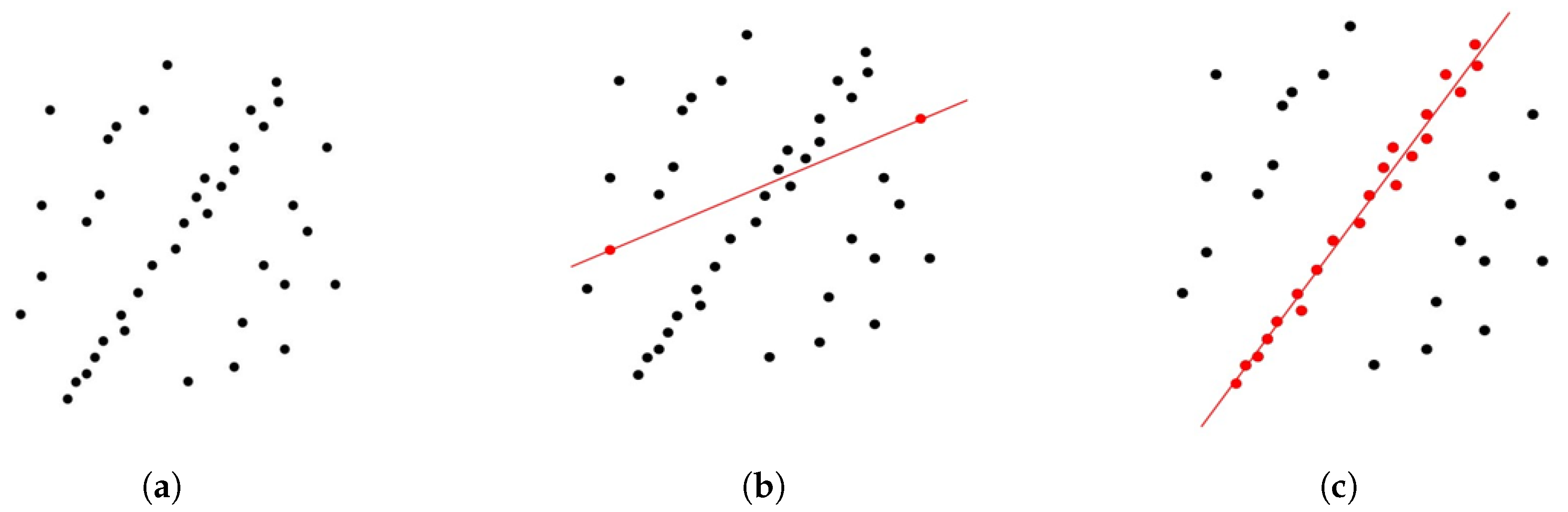
• These steps are repeated until either a predefined maximum number of iterations is reached or the best model satisfying the criteria is found. After completing all iterations, the best model is output.

Figure 1 illustrates the iterative process and results of RANSAC. In a two-dimensional dataset containing outliers, RANSAC iteratively refines its fitting, accurately fitting a line that reflects the overall trend of the dataset while effectively eliminating the interference of outliers, thereby ensuring the fitting accuracy of the line model.

3. Modified Random Sample Consensus-Based Linear Fitting Algorithm

3.1. Locality-Sensitive Hashing

In the field of outlier data processing, effectively obtaining and analyzing the correlation information between data in high-dimensional space is crucial. Given that the correlation among data can be translated into neighborhood relationships, the local vicinity information of the data can be leveraged to deduce the associations between data points. Hashing techniques represent a common method for approximate nearest neighbor searches. The method first identifies a hash function that maps similar data points to the same hash table, and then performs a data search around the query position in the hash table to find the nearest neighbors of the target data. Among these, Locality-Sensitive Hashing is one of the most commonly used methods. The core idea of LSH is that in high-dimensional space, if two data points are close to each other, the hash function is likely to produce the same hash values for them with a high probability; conversely, for points that are not close together, the hash function tends to generate different hash values with a high probability. LSH is a hashing technique designed for efficient approximate nearest neighbor search, focusing on constructing a family of hash functions that preserve the similarity between points. In the context of line fitting, the similarity between points is typically measured using Euclidean distance or cosine similarity. For data points v in the dataset, let $v_i(x_i,y_i)$ and $v_j(x_j,y_j)$ represent a pair of points. The formulas for Euclidean distance and cosine similarity are given by Equations (10) and (11), respectively.

$$\parallel v_i-v_j{\parallel }^2=\sqrt{{(x_i-x_j)}^2+{(y_i-y_j)}^2}$$

(10)

$$sim(v_i,v_j)={\displaystyle \frac{v_i{v}_j}{\parallel v_i\parallel \parallel v_j\parallel }}$$

(11)

Construct a family of hash functions $\mathcal{H}$ that satisfies the locality-sensitive property, such that similar points are mapped into the same bucket with a high probability, while dissimilar points are mapped into the same bucket with a low probability.

In two-dimensional or higher-dimensional spaces, the distribution of data points is often quite complex, necessitating the design of effective hash functions that ensure that highly similar data points are mapped to the same bucket, while less similar data points are mapped to different buckets. One approach to designing hash functions is through random hyperplane projection, where the basic idea is to use hyperplanes to divide the space into two parts, with the projection of data points on the hyperplane determining their hash values. By constructing multiple random hyperplanes, data points are projected onto multiple hash values, thereby improving classification accuracy.

The specific process of Locality-Sensitive Hashing for finding similar data is as follows:

• Construct appropriate locality-sensitive hash functions to ensure that similar data points are mapped into the same or adjacent hash buckets.
• Utilize the constructed hash functions to map all data points in the dataset into their corresponding buckets in the hash table, with each bucket containing similar data points.
• Retrieve points mapped to the same or adjacent buckets, treating these points as candidate neighbors. By further calculating the similarities of these candidate points, the final neighbors can be determined.

3.2. Random Sample Consensus Based on Locality-Sensitive Hashing Algorithm

The LSH-RANSAC algorithm combines the efficient similarity search of LSH with the robust fitting mechanism of RANSAC, aiming to quickly eliminate outliers in the data and accurately fit the best model. For the observed dataset $D=(x_i,y_i)$, the goal is to fit a line model $y=ax+b$. The specific process for fitting the linear parameter model using the LSH-RANSAC algorithm is as follows:

• The hash function based on random hyperplanes is given by

  $$h\left(x\right)=sgn(x·\nu )$$

  (12)

  where $\nu$ is a two-dimensional random vector, with each component independently following a standard normal distribution $N(0,1)$, and $x·\nu$ is the projection of x onto $\nu$. The sgn function is defined as:

  $$sgn\left(x\right)=\left\{\begin{array}{cc}1,\hfill & \mathrm{if}x⩾0\hfill \\ 0,\hfill & \mathrm{if}x<0\hfill \end{array}\right.$$

  (13)
  The similarity between two points can be represented using the Euclidean distance function. The hash function projects data points into hash buckets via random hyperplane projections, with the Euclidean distance determining whether the projections of the data points are similar. The Euclidean distance formula in two-dimensional space is given by

  $$d(x,y)=\sqrt{{(x_1-y_1)}^2+{(x_2-y_2)}^2}$$

  (14)
  In this equation, a smaller value of (d(x,y)) indicates a higher similarity between the data points, increasing the probability that they share the same hash value.
• To enhance the effective mapping of similar data points into the same hash bucket, multiple hash functions are typically employed, representing data points as a vector of multiple binary bits:

  $$b\left(x_i\right)=\{h_1\left(x_i\right),h_2\left(x_i\right),\dots ,h_k\left(x_i\right)\}\in {\{0,1\}}^k$$

  (15)

  where k is the number of hash functions. After random hyperplane projection, for the dataset $D=(x_i,y_i)$, we obtain the corresponding binary vector set B:

  $$B=\left[\begin{array}{c}b\left(x_1\right)\\ b\left(x_2\right)\\ ⋮\\ b\left(x_i\right)\end{array}\right]=\left[\begin{array}{cccc}{h}_1\left(x_1\right)& h_2\left(x_1\right)& \dots & h_k\left(x_1\right)\\ h_1\left(x_2\right)& h_2\left(x_2\right)& \dots & h_k\left(x_2\right)\\ ⋮& ⋮& \ddots & ⋮\\ h_1\left(x_i\right)& h_2\left(x_i\right)& \dots & h_k\left(x_i\right)\end{array}\right]$$

  (16)
• A threshold T is set, and for each data point $x_i$, the number of similar data points, i.e., the number of neighbors $N\left(x_i\right)$ is computed. If $N\left(x_i\right)<T$, the data point is considered an outlier and is removed. The resulting processed dataset is $D^{\prime }=\left\{(x_i^{\prime },y_i^{\prime })\right\}$.
• From the processed dataset $D^{\prime }=\left\{(x_i^{\prime },y_i^{\prime })\right\}$, a minimal sample set is randomly selected. For line fitting, the minimal sample set requires two data points.
• The selected subset is used to fit the line model $y=ax+b$, and the model parameters a and b are computed using the following formulas:

  $$a={\displaystyle \frac{n{\sum }_{i=1}^n{x}_i{y}_i-{\sum }_{i=1}^n{x}_i{\sum }_{i=1}^n{y}_i}{n{\sum }_{i=1}^n{x}_i^2-{\left({\sum }_{i=1}^n{x}_i\right)}^2}}$$

  (17)

  $$b={\displaystyle \frac{{\sum }_{i=1}^n{y}_i-a{\sum }_{i=1}^n{x}_i}{n}}$$

  (18)
  The distance $d_i$ from each point in the dataset to the current fitted line is calculated as

  $$d_i={\displaystyle \frac{|a{x}_i+b-y_i|}{\sqrt{a^2+1}}}$$

  (19)
• A threshold $\theta$ is defined to check whether the distance $d_i$ from each point to the fitted line is less than $\theta$. If $d_i<\theta$, the data point is an inlier, and the number of inliers for each iteration is recorded. If the number of inliers in this iteration exceeds that of the previous iteration, the model parameters are updated.
• Steps 5 to 7 are repeated, each time selecting a new subset for model fitting until either the maximum iteration count is reached or the current line model fit is deemed satisfactory (i.e., the number of inliers reaches the predefined threshold T). In order to ensure the identification of an appropriate line model, the maximum iteration count K is calculated as follows:

  $$K={\displaystyle \frac{log(1-p)}{log(1-w^n)}}$$

  (20)

  where p is the probability of finding a reliable model, and $w^n$ is the probability that all n randomly selected points are inliers.
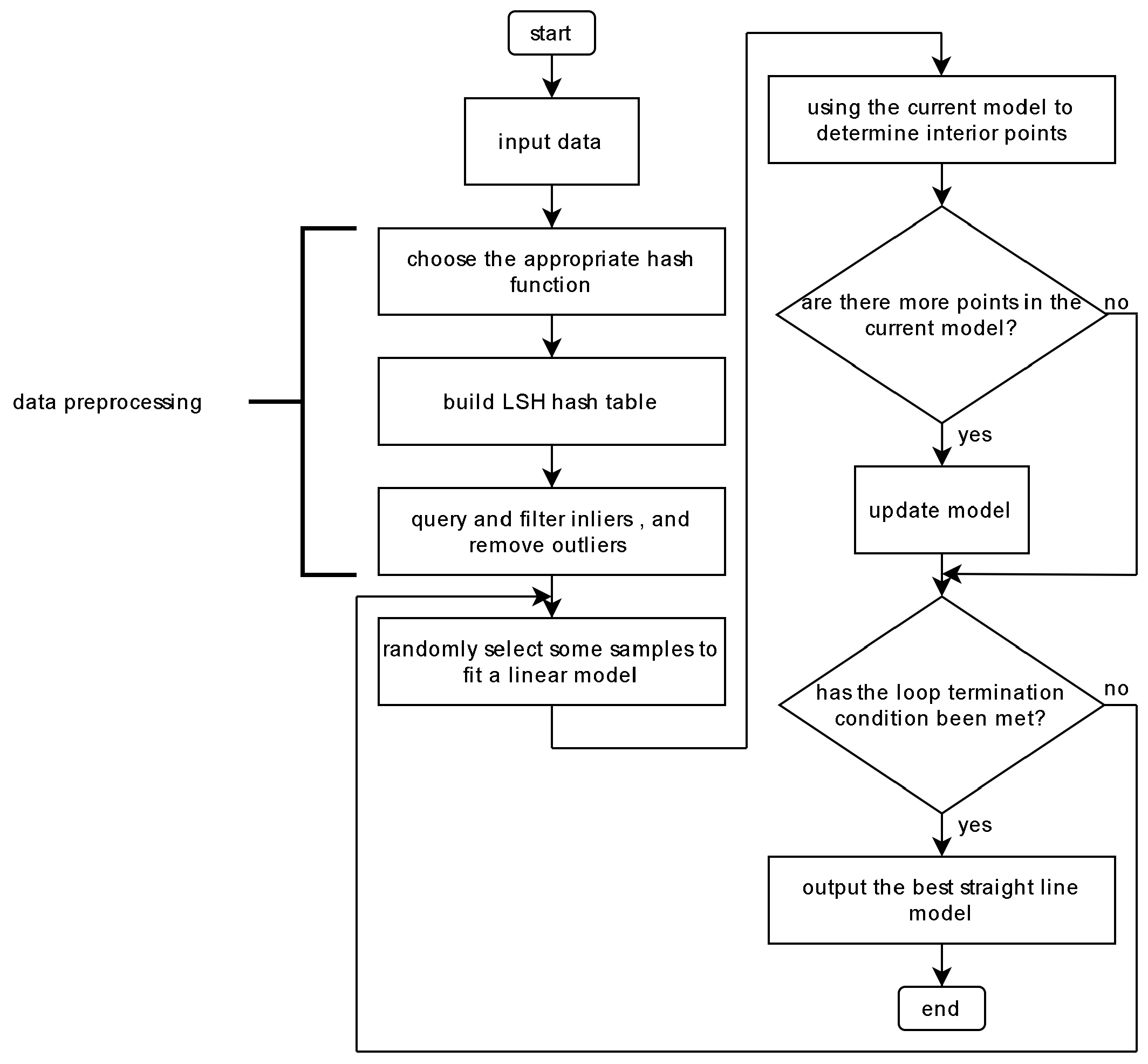
• After completing all iterations, the line model with the highest number of inliers is output as the final fitting result. The flowchart of the LSH-RANSAC algorithm is shown in Figure 2.

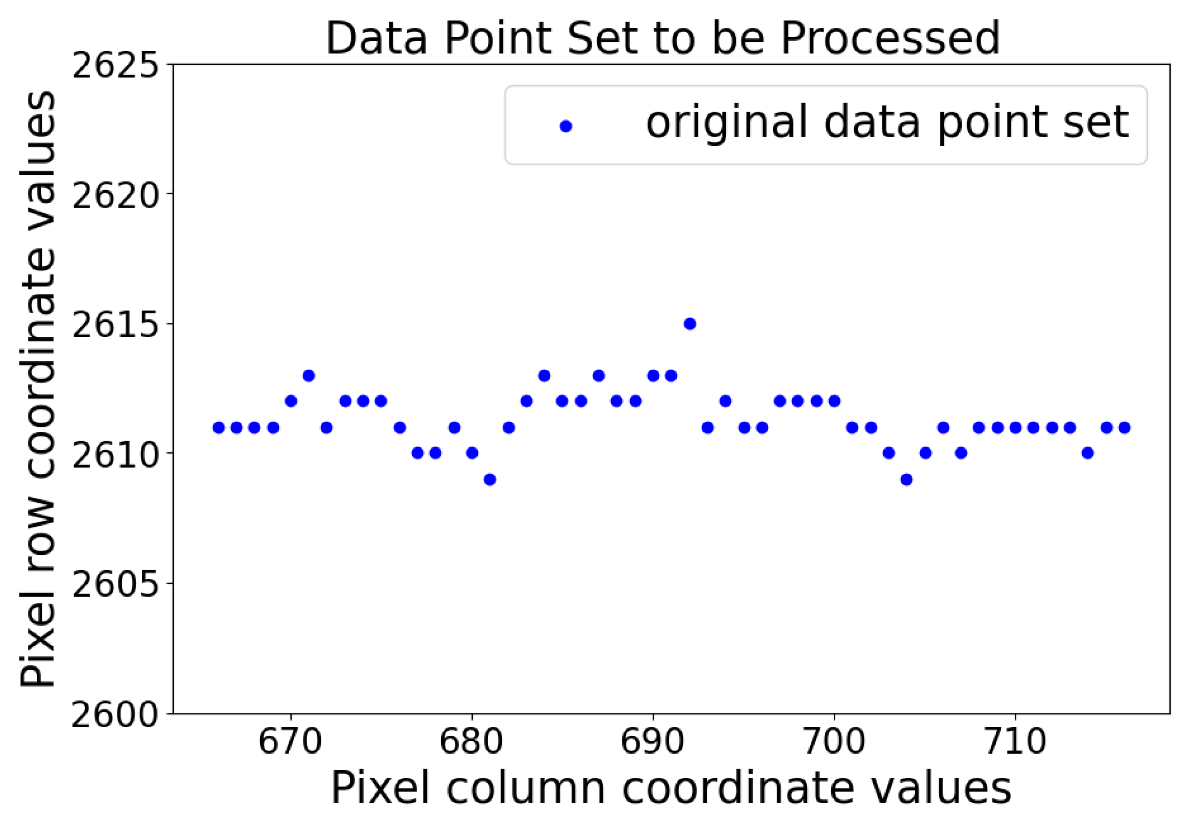
As illustrated in Figure 3, given a set of observed data points, this dataset represents the center point coordinates of a line laser stripe image, with the x-axis data as pixel column coordinates and the y-axis data as pixel row coordinates. The objective is to fit an appropriate line from these observation data points that accurately reflects the trend of the valid data. This dataset contains a certain number of interfering noise points (i.e., outliers), which deviate from the true line and can reduce the fitting accuracy of the model. The LSH-RANSAC algorithm is employed to eliminate the outliers and fit the line model parameters from the processed dataset.

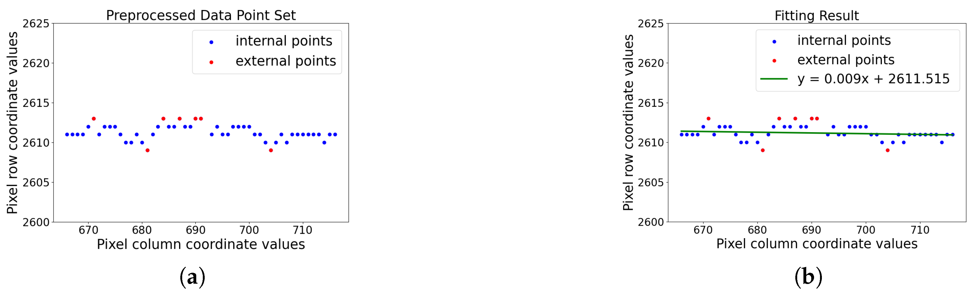
Figure 4 displays the results of fitting the observed data point set using the LSH-based RANSAC algorithm, with the fitted line model’s slope a being −0.009 and the intercept b being 2617.515.

4. Algorithm Verification and Discussion

To evaluate the performance of the proposed algorithm, the LSH-RANSAC algorithm was compared with the WLS, RANSAC, and MLE. The validation of the algorithm is implemented in Python (with version 3.12) by importing the MinHash and MinHashLSH functions from the datasketch package. In the MinHashLSH algorithm, there is no strict requirement on the specific types of hash functions, and it is not necessary to specify a particular function type during application. By selecting a sufficient number of hash functions, the accuracy of the MinHash algorithm in estimating set similarity can be improved. In this study, the number of hash functions used is 128, the Jaccard similarity threshold is set to 0.9, and the maximum number of iterations is set to 2000.

4.1. Technical Indicators

After fitting the line models using the various algorithms, their performance should be accessed based on several technical metrics, including the Residual Sum of Squares (RSS), the coefficient of determination $R^2$, and the Mean Absolute Error (MAE).

• The RSS quantifies the squared differences between the observed values and the predicted values, reflecting the degree of deviation between the model and the data. A smaller RSS indicates a better model fit and improved predictive capability. The RSS is defined as follows:

  $$\mathrm{RSS}=\sum _{i=1}^n{(y_i-{\widehat{y}}_i)}^2$$

  (21)

  where $y_i$ represents the actual values and ${\widehat{y}}_i$ denotes the predicted values.
• The coefficient of determination $R^2$, also known as the goodness-of-fit statistic, reveals the extent to which the independent variables can explain or predict the variation in the dependent variable. The value of $R^2$ ranges from 0 to 1: a value close to 1 suggests an excellent model fit and a strong explanation of the data’s variance, while a value close to 0 indicates poor explanatory power regarding the changes in the dependent variable. The $R^2$ is calculated based on the relationship between the RSS and the total sum of squares, defined as

  $$R^2=1-{\displaystyle \frac{RSS}{TSS}}=1-{\displaystyle \frac{{\sum }_{i=1}^n{(y_i-{\widehat{y}}_i)}^2}{{\sum }_{i=1}^n{(y_i-{\overline{y}}_i)}^2}}$$

  (22)

  where $\overline{y}$ is the mean of the data.
• The MAE measures the average magnitude of the errors in predictions, with smaller errors indicating greater accuracy. The MAE is defined as follows:

  $$\mathrm{MAE}={\displaystyle \frac{1}{n}}\sum _{i=1}^n|y_i-{\widehat{y}}_i|$$

  (23)

4.2. Simulation Results

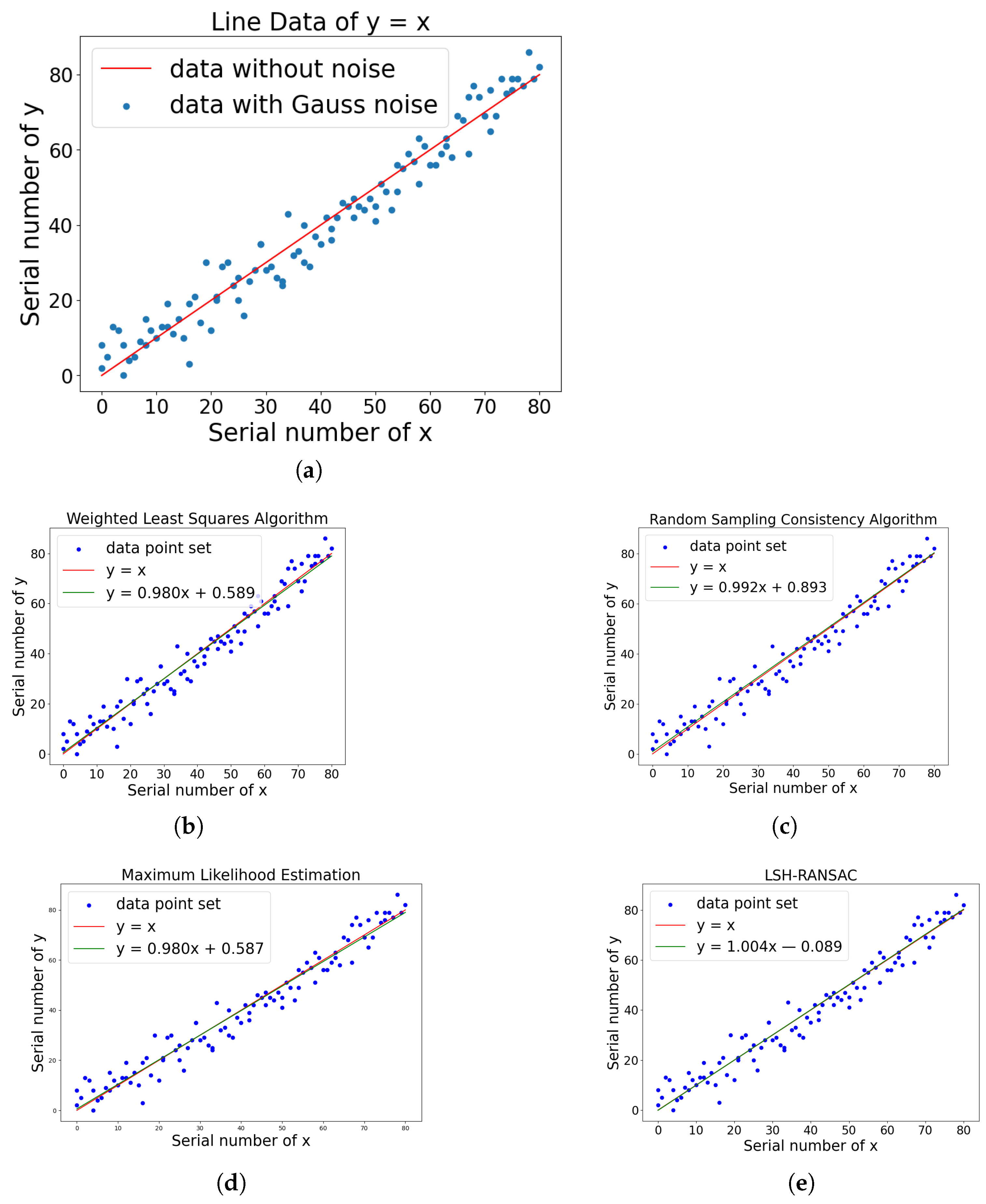
To given a brief verification of our algorithm, we first set a line $y=x$ with extra Gaussian noises, e.g., the parameters of the original line are $a=1$ and $b=0$ as shown in Figure 5a.

Here the blue points are the line data with extra noise added. The Gaussian noise in the simulation has the expectation value 0 and variance 5. Figure 5b–e show the line fitting results with related algorithm. The LSH-RANSAC algorithm proposed in this paper fits a line that nearly perfectly coincides with the standard original line, while the fitting results of the other three algorithms exhibit minor deviations. The fitting results of all four algorithms are summarized in

Table 1. Comparison between our methods and commonly used ones.

	WLS	RANSAC	MLE	LSH-RANSAC
Fitted (a,b)	(0.980,0.589)	(0.992,0.893)	(0.980,0.587)	(1.004,−0.089)
Euclidean distance	0.589	0.893	0.587	0.089

.

The proposed LSH-RANSAC algorithm fits a line that almost perfectly coincides with the original line, while the fitting results of the other three algorithms exhibit minor deviations.

In a real dataset fitting experiment, the dataset consists of the center points extracted from a specific laser stripe, as illustrated in Figure 6a. Figure 6b–e show the line-fitting results obtained by each algorithm.

The technical metrics for each algorithm in fitting the given point set are summarized in

Table 2. Technical indicators of each algorithm fitting the target data set.

Technical Indicator	WLS	RANSAC	MLE	LSH-RANSAC
RSS	66.276	55.678	50.742	46.613
$R^2$	0.724	0.813	0.857	0.898
MAE	0.498	0.412	0.386	0.287

.

As shown in Table 2, compared to the WLS, RANSAC, and MLE methods, the LSH-RANSAC algorithm demonstrates lower values for both the Mean Absolute Error and Residual Sum of Squares, alongside a higher coefficient of determination. This indicates that the LSH-RANSAC algorithm is more effective at mitigating the influence of outliers when fitting datasets that contain such anomalies, resulting in superior fitting performance.

4.3. Analysis

When processing simulated data, the parameters fitted by the WLS, RANSAC, MLE, and the LSH-RANSAC algorithm exhibit Euclidean distances to the standard line parameters of 0.589, 0.893, 0.587, and 0.089, respectively. The Euclidean distance obtained by the LSH-RANSAC algorithm is significantly lower than that of the other three fitting algorithms, indicating its superior fitting performance. This improvement is attributed to the introduction of locality-sensitive hash functions, which reduces the influence of outliers on the fitting results.

In the case of real data, the LSH-RANSAC algorithm achieved a reduction of 29%, 16%, and 8% in the sum of squared residuals compared to the other three algorithms, while the coefficient of determination increased by 24%, 10%, and 5%, respectively. Additionally, the mean absolute error decreased by 42%, 30%, and 26%, demonstrating substantial improvements across all metrics.

The mimic simulation validation may lose the ability to reveal potential bias problems when Gaussian noise was added. Although minor deviations did not affect the overall results which were observed at different noise parameters, the bias in real environment might not be displaced as balanced noise. There are inherent differences between simulated data and real data; the added noise is randomly distributed on both sides of the standard line, while the distribution of outliers in real data points may vary. Our algorithm thus perform a better solution for actual situations.

Since different parameters, such as the number of hash functions, similarity threshold, and the number of iterations, may lead to varying computation times. In applications that require real-time processing, it is essential to adjust the algorithm parameters to better suit the data being processed. This paper does not conclude the time consumption of the algorithm, due to the varying parameters may cause huge difference. Furthermore, recent studies integrating deep learning with RANSAC algorithms may require more processing time than our classical algorithm.

5. Conclusions

This paper proposes an improved line fitting algorithm based on RANSAC. The LSH-based RANSAC algorithm combines the efficient similarity search capabilities of LSH with the robust fitting mechanism of RANSAC. This approach enables the rapid elimination of outliers in the data while accurately fitting the optimal model. The algorithm possesses the following characteristics: (1) Improved Fitting Accuracy. By introducing LSH, the algorithm utilizes the locality-sensitive nature of LSH to eliminate outliers before fitting, thereby reducing the impact of these outliers on the fitting results. (2) The algorithm further employs the iterative nature of RANSAC, selectively filtering inliers and outliers during each fitting iteration based on the model’s adaptability, thereby progressively approximating the optimal model. (3) Enhanced Robustness. The locality-sensitive property of LSH also helps to filter out the influence of noise and outliers on the dataset, making the RANSAC algorithm more stable and reliable during the model fitting process. This enhancement allows the algorithm to better handle datasets containing noise and outliers, thereby increasing its applicability.

Experimental results demonstrate that the proposed improved RANSAC line fitting algorithm significantly outperforms WLS, RANSAC, and MLE. When fitting simulation datasets, the fitted curve nearly coincided with the known line, and the Euclidean distance between the result parameters and the known standard parameters for the LSH-RANSAC algorithm was merely 0.089, far lower than that of the other three fitting algorithms. When fitting the real target dataset, the LSH-RANSAC algorithm shows substantial improvements across all three technical metrics compared to the other three algorithms.

The research findings have been applied in a project focused on ultrathin thickness measurement of objects using modulation line lasers, yielding high measurement accuracy that meets the requirements and demonstrates substantial practical application value. Future work may further investigate the influence of different hash functions within the Local Sensitive Hashing framework on the processing of outcomes for various types of data, enhancing the algorithm’s robustness.

The LSH-RANSAC algorithm is proposed to handle a specific linear fitting scene with a two-dimensional database and low time sensitivity; thus, we do not validate the algorithm’s performance on datasets with a high proportion of outliers, the execution times, nor the algorithm’s effectiveness in higher dimensional spaces. Future research can be further developed based on the following aspects: (1) Investigate the algorithm’s performance when there is a significant proportion of outliers in the dataset to figure out its effectiveness. (2) When handling data with high time sensitivity, analyze the algorithm’s computational complexity and measure the execution time to ensure real-time processing requirements are met. (3) Validate the effectiveness of the algorithm when applied to high-dimensional data. (4) Study the impact of adjusting various parameters of the LSH algorithm on the results obtained for different types of data, aiming to further enhance the robustness of the algorithm.

References

- Prieto-Fernández, N.; Fernández-Blanco, S.; Fernández-Blanco, A.; Benítez-Andrades, J.A.; Carro-De-Lorenzo, F.; Benavides, C. Conditional Weighted Linear Fitting for 2D-LiDAR-Mapping of Indoor SLAM. IEEE Trans. Ind. Inform. 2024, 20, 9579–9587. [Google Scholar] [CrossRef]
- You, H.; Xie, Y. Automatic driving image matching via Random Sample Consensus (RANSAC) and Spectral Clustering (SC) with monocular camera. Rev. Sci. Instrum. 2024, 95, 085113. [Google Scholar] [CrossRef] [PubMed]
- Guo, R.; Liu, S.; He, Y.; Xu, L. Study on Vehicle–Road Interaction for Autonomous Driving. Sustainability 2022, 14, 11693. [Google Scholar] [CrossRef]
- Elberink, S.; Khoshelham, K. Automatic Extraction of Railroad Centerlines from Mobile Laser Scanning Data. Remote Sens. 2015, 7, 5565–5583. [Google Scholar] [CrossRef]
- Mohiuddin, A.M.; Bansal, J.C. An improved linear prediction evolution algorithm based on nonlinear least square fitting model for optimization. Soft Comput. 2023, 27, 14019–14044. [Google Scholar] [CrossRef]
- Dai, C.; Hu, Z.; Li, Z.; Xiong, Z.; Su, Q. An Improved Grey Prediction Evolution Algorithm Based on Topological Opposition-Based Learning. IEEE Access 2020, 8, 30745–30762. [Google Scholar] [CrossRef]
- Ghadhban, H.Q.; Othman, M.; Samsudin, N.; Kasim, S.; Mohamed, A.; Aljeroudi, Y. Segments Interpolation Extractor for Finding the Best Fit Line in Arabic Offline Handwriting Recognition Words. IEEE Access 2021, 9, 73482–73494. [Google Scholar] [CrossRef]
- Yao, S.; Zhang, Y.; Xu, Y.; Gu, Y.; Wu, Q.; Liu, X. An improved parameter estimation of HFM signals based on IRLS linear fitting of extracted group delay. Signal Process. 2024, 217, 109347. [Google Scholar] [CrossRef]
- Yuan, Y.; Yu, M.; Wang, W.; Xing, B. Machine Learning Based Linear Fitting of Wind Direction and Speed. In Proceedings of the 2023 6th International Conference on Electronics Technology (ICET), Chengdu, China, 12–15 May 2023; pp. 1134–1139. [Google Scholar] [CrossRef]
- Yan, J.; Tao, C.; Wang, Y.; Du, J.; Qi, M.; Zhang, Z.; Hu, B. Application of Enhanced Weighted Least Squares with Dark Background Image Fusion for Inhomogeneity Noise Removal in Brain Tumor Hyperspectral Images. Appl. Sci. 2024, 15, 321. [Google Scholar] [CrossRef]
- Koci, J.; Panou, G. Techniques for Least-Squares Fitting of Curves and Surfaces to a Large Set of Points. J. Surv. Eng. 2025, 151, 04024018. [Google Scholar] [CrossRef]
- Gu, J.; Kong, X.; Guo, J.; Qi, H.; Wang, Z. Parameter estimation of three-parameter Weibull distribution by hybrid gray genetic algorithm with modified maximum likelihood method with small samples. J. Mech. Sci. Technol. 2024, 38, 5363–5379. [Google Scholar] [CrossRef]
- Fischler, M.A.; Bolles, R.C. Random sample consensus: A paradigm for model fitting with applications to image analysis and automated cartography. Commun. ACM 1981, 24, 381–395. [Google Scholar] [CrossRef]
- Raguram, R.; Frahm, J.M.; Pollefeys, M. A Comparative Analysis of RANSAC Techniques Leading to Adaptive Real-Time Random Sample Consensus. In Computer Vision–ECCV 2008; Springer: Berlin/Heidelberg, Germany, 2008; pp. 500–513. [Google Scholar] [CrossRef]
- Gao, Y.; Fu, J.; Chen, X. Correcting Hardening Artifacts of Aero-Engine Blades with an Iterative Linear Fitting Technique Framework. Sensors 2024, 24, 2001. [Google Scholar] [CrossRef] [PubMed]
- Sa, J.; Ding, L.; Huang, Y. LS-RANSAC: Find spatial structures directly from the image. Signal Image Video Process. 2025, 19, 413. [Google Scholar] [CrossRef]
- Lin, X.; Zhou, Y.; Liu, Y.; Zhu, C. A Comprehensive Review of Image Line Segment Detection and Description: Taxonomies, Comparisons, and Challenges. IEEE Trans. Pattern Anal. Mach. Intell. 2024, 46, 8074–8093. [Google Scholar] [CrossRef]
- Zhang, H.; Liang, J.; Jiang, H.; Cai, Y.; Xu, X. Lane line recognition based on improved 2D-gamma function and variable threshold Canny algorithm under complex environment. Meas. Control 2020, 53, 1694–1708. [Google Scholar] [CrossRef]
- Yang, Y.G.; Zhang, S.M.; Jiang, D.H.; Liao, X. Image retrievable encryption based on linear fitting and orthogonal transformation. Phys. Scr. 2024, 100, 015213. [Google Scholar] [CrossRef]
- Cheng, D.; Huang, J.; Zhang, S.; Wu, Q. A robust method based on locality sensitive hashing for K-nearest neighbors searching. Wirel. Netw. 2022, 30, 4195–4208. [Google Scholar] [CrossRef]
- Mu, Z.; Liu, Y.; Yang, Y. A large-scale group decision making model with a clustering algorithm based on a locality sensitive hash function. Eng. Appl. Artif. Intell. 2025, 140, 109697. [Google Scholar] [CrossRef]
- Donadi, I.; Pretto, A. KVN: Keypoints Voting Network with Differentiable RANSAC for Stereo Pose Estimation. IEEE Robot. Autom. Lett. 2024, 9, 3498–3505. [Google Scholar] [CrossRef]
- Kone, S.; Sere, A.; Somda, D.A.M.; Ouedraogo, J.A. A Framework for Age Estimation of Fish from Otoliths: Synergy Between RANSAC and Deep Neural Networks. Int. J. Adv. Comput. Sci. Appl. 2024, 15, 925–932. [Google Scholar] [CrossRef]
- Santarossa, M.; Koch, R.; Tavakoli, M. Robust Multimodal Retinal Image Registration in Diabetic Retinopathy Using a Lightweight Neural Network and Improved RANSAC Algorithm. IEEE Sens. J. 2025, 25, 13469–13479. [Google Scholar] [CrossRef]
- Saeki, K.; Tanaka, K.; Ueda, T. LSH-RANSAC: An incremental scheme for scalable localization. In Proceedings of the 2009 IEEE International Conference on Robotics and Automation, Kobe, Japan, 12–17 May 2009; IEEE: Piscataway, NJ, USA, 2009; pp. 3523–3530. [Google Scholar] [CrossRef]
- Tanaka, K.; Saeki, K.i.; Minami, M.; Ueda, T. LSH-RANSAC: Incremental Matching of Large-Size Maps. IEICE Trans. Inf. Syst. 2010, 93, 326–334. [Google Scholar] [CrossRef]