Enhancing Sign Language Recognition Performance Through Coverage-Based Dynamic Clip Generation

Abstract

Sign Language Recognition (SLR) has made substantial progress through advances in deep learning and video-based action recognition. Conventional SLR systems typically segment input videos into a fixed number of clips (e.g., five clips per video), regardless of the video’s actual length, to meet the fixed-length input requirements of deep learning models. While this approach simplifies model design and training, it fails to account for temporal variations inherent in sign language videos. Specifically, applying a fixed number of clips to videos of varying lengths can lead to significant information loss: longer videos suffer from excessive frame skipping, causing the model to miss critical gestural cues, whereas shorter videos require frame duplication, introducing temporal redundancy that distorts motion dynamics. To address these limitations, we propose a dynamic clip generation method that adaptively adjusts the number of clips during inference based on a novel coverage metric. This metric quantifies how effectively a clip selection captures the temporal information in a given video, enabling the system to maintain both temporal fidelity and computational efficiency. Experimental results on benchmark SLR datasets using multiple models-including 3D CNNs, R(2+1)D, Video Swin Transformer, and Multiscale Vision Transformers demonstrate that our method consistently outperforms fixed clip generation methods. Notably, our approach achieves 98.67% accuracy with the Video Swin Transformer while reducing inference time by 28.57%. These findings highlight the effectiveness of coverage-based dynamic clip generation in improving both accuracy and efficiency, particularly for videos with high temporal variability.

1. Introduction

Sign language (SL) is an essential means of communication for people with hearing impairments and serves as a bridge between the Deaf and non-Deaf communities. With recent advances in artificial intelligence, deep learning-based sign language recognition (SLR) has gained significant attention, leading to the development of various translation systems [1,2,3,4,5]. In addition to these developments, recent studies have explored sign language recognition in mobile environments, making communication more accessible and convenient [6,7,8,9]. While these technologies enhance communication accessibility, research on optimizing and improving the performance of sign language recognition systems remains limited, particularly in terms of model recognition accuracy and inference speed.

To enhance the accuracy of sign language recognition (SLR), videos are commonly segmented into multiple clips for model processing. This multi-clip approach is widely adopted across video recognition as it demonstrably optimizes computational efficiency and recognition accuracy by enabling models to effectively capture temporal dynamics within manageable computational constraints [10,11,12]. In deep learning-based SLR systems, this segmentation addresses a fundamental requirement: these models typically operate on fixed-length sequences of image frames as input. Consequently, dividing videos into multiple segments becomes necessary to conform to these architectural constraints.

Nonetheless, conventional approaches that segment videos into a predetermined and fixed number of clips present inherent limitations. In the case of longer sign language videos, such fixed partitioning often leads to excessive frame skipping, thereby omitting essential gestural cues crucial for accurate recognition. Conversely, shorter videos may necessitate frame duplication to meet input length requirements, introducing redundancy and degrading model performance. These constraints underscore the necessity for a more adaptive and content-aware clip generation strategy that can dynamically adjust to the temporal characteristics of each video.

To address the aforementioned limitations, we propose a dynamic clip generation method that adjusts the number of clips during inference based on a novel coverage metric. This metric reflects how effectively temporal information is captured from the video. Our method dynamically determines the number of clips based on video length, ensuring sufficient context for long videos while avoiding redundancy in short ones. While a full discussion of model-specific performance is provided in the conclusion, the proposed dynamic clip generation method enhances sign language recognition accuracy while minimizing inference time overhead.

The main contributions of this study are as follows:

• Dynamic Clip Generation Based on Coverage: We propose a novel dynamic clip generation method that adjusts the number of clips during inference based on a proposed coverage metric. This metric reflects how effectively temporal information is captured from sign language videos, enabling adaptive clip generation tailored to each video’s length and temporal complexity.
• Improved Trade-off Between Accuracy and Inference Time: Through extensive experiments on various SLR models, including 3D CNN, R(2+1)D, Video Swin Transformer (VST), and Multiscale Vision Transformers (MViT), we demonstrate that our dynamic method achieves a better trade-off between computational efficiency and recognition accuracy compared to fixed clip generation methods.
• Empirical Validation of the Coverage Metric: We conduct a quantitative analysis by varying the number of clips and measuring the corresponding coverage values. The results show that maintaining a coverage value of at least 1 is essential for preserving contextual information, while excessive redundancy can be avoided through our dynamic method.
• General Applicability Across Architectures: Our method consistently improves or maintains performance across a range of model architectures. Notably, it achieves significant reductions in inference time for models such as 3D CNN, R(2+1)D, and VST without compromising accuracy.

The remainder of this paper is structured as follows. Section 2 reviews related work. Section 3 presents our proposed method. Section 4 describes the experimental setup and discusses the results. Section 5 concludes the paper with key findings and future research directions.

2. Related Works

In this section, we review relevant research on efficient video processing for sign language recognition and related domains. We categorize the existing works into three main themes: frame and resolution optimization, adaptive sampling and keypoint detection, and multimodal and hybrid approaches.

Table 1. Frame and resolution optimization techniques.

Researcher	Key Techniques
Lianyu Hu et al. [13]	AdaBrowse: Selectively processes only the most informative parts of the video, reducing computational cost while maintaining recognition accuracy
Lianyu Hu et al. [14]	Dynamic Resolution Adjustment: Dynamically adjusts input frame resolution to reduce computational cost and time
Yongquan Shao et al. [15]	Key Frame Extraction + TSM: Selects frames based on inter-frame difference and uses time-shift modules to model temporal features with reduced overhead
Zhen Wang et al. [16]	STNet: Enhances temporal consistency and frame-wise distinctiveness using optimal transport, frame-wise loss, and multi-scale temporal fusion

summarizes key research focused on frame and resolution optimization techniques.

Lianyu Hu et al. proposed a method that reduces computational cost while maintaining recognition accuracy by selecting only the most informative video segments. A lightweight network extracts coarse features, and a policy network dynamically selects key subsequences for processing, thereby reducing redundant computation. Furthermore, the adaptive model AdaBrowse improves efficiency by adjusting the input resolution based on spatial redundancy, achieving state-of-the-art performance with lower FLOPs [13].

For continuous sign language recognition, Lianyu Hu et al. also introduced a scalable frame resolution approach that dynamically adjusts resolution based on task context. By lowering the resolution when high detail is unnecessary, the method improves processing speed without compromising accuracy, making real-time CSLR systems more efficient [14].

Yongquan Shao et al. proposed a time-efficient sign language recognition approach by combining key frame extraction with temporal shift modeling. Their method uses the inter-frame difference technique to identify motion-salient frames, thereby avoiding the need to process full-length videos. The selected frames are then passed through a ResNet50 backbone integrated with the Temporal Shift Module (TSM), allowing for temporal modeling across frames with minimal additional computation. This approach achieves state-of-the-art accuracy on Chinese Sign Language datasets while significantly reducing the number of processed frames and parameters [15].

Zhen Wang et al. proposed a novel framework called STNet, which enhances spatio-temporal feature representation through frame-level optimization techniques. Their method introduces a Spatial Resonance Module (SRM) that employs the Sinkhorn–Knopp algorithm to model feature transport between adjacent frames, thereby improving the continuity and consistency of extracted features. To preserve frame-specific details, they also propose a frame-wise loss function that enhances feature discriminability across frames. Furthermore, the Multi-Temporal Perception Module (MTPM) aggregates features at multiple temporal scales, enabling effective modeling of both short- and long-term dependencies. STNet demonstrates competitive performance across multiple CSLR benchmarks while maintaining high efficiency through reduced frame redundancy [16].

Table 2. Adaptive sampling and keypoint detection techniques.

Researcher	Key Techniques
Geunmo Kim et al. [17]	Keypoint-Based Sign Language Start and End Point Detection: Extracts keypoint information, monitors changes over time, and applies thresholding to detect gesture boundaries with high accuracy
Taewan Kim et al. [18]	Dynamic Sampling Rate Adjustment: Dynamically adjusts the sampling rate based on the frame rate in real-time to improve recognition accuracy in a mobile environment
Zheng et al. [19]	Dynamic Sampling Network: Dynamically selects important clips during both training and inference to reduce computational cost while maintaining performance
Afham et al. [20]	Kernel Temporal Segmentation: Divides videos into semantically consistent segments and samples frames from each segment
Zuo et al. [21]	Keypoint-Guided Spatial Attention: Utilizes pose keypoint heatmaps to enhance the visual module’s focus on informative regions (face and hands), improving recognition accuracy in continuous sign language recognition (CSLR)

summarizes the research focused on adaptive sampling and keypoint detection techniques.

Geunmo Kim et al. introduced a novel keypoint-based approach for detecting the start and end points of sign language gestures. Their method extracts keypoint information from signers and monitors changes in these keypoints over time to identify gesture boundaries. By applying a threshold-based technique to the average keypoint change, the system accurately determines when a sign begins and ends. Experimental results demonstrate that using ten keypoints enables precise boundary detection within approximately two frames, thereby improving the overall accuracy of sign language recognition. This approach underscores the importance of temporal keypoint analysis in enhancing recognition performance [17].

Taewan Kim et al. proposed a dynamic sampling rate adjustment method that detects the boundaries of sign language utterances and adjusts the frame extraction rate accordingly, based on the number of sign language image frames that can be acquired per unit time. This dynamic approach improves the recognition accuracy across devices with varying computational capabilities, achieving up to 66.54% higher Top-1 accuracy and 83.64% higher Top-5 accuracy compared to the fixed sampling rate method [18].

Zheng et al. introduced the Dynamic Sampling Network (DSN), which optimally selects video clips during both training and inference using reinforcement learning. Unlike traditional fixed clip sampling methods, the DSN learns to focus on key segments, reducing computational cost while maintaining accuracy [19]

Afham et al. proposed the Kernel Temporal Segmentation (KTS), an adaptive frame sampling method that decomposes long videos into semantically consistent segments. By leveraging frame-to-frame similarity analysis, KTS outperforms uniform sampling, enhancing both video classification and temporal action localization performance [20].

Zuo et al. introduced a keypoint-guided spatial attention module to enhance visual feature extraction in continuous sign language recognition (CSLR). By leveraging pose keypoint heatmaps, their method dynamically focuses on informative regions such as the face and hands, thereby improving recognition accuracy while maintaining computational efficiency. This Spatial Attention Consistency (SAC) technique strengthens the model’s ability to detect critical movements essential for sign language recognition [21].

Table 3. Multimodal and hybrid approaches.

Researcher	Key Techniques
Wei et al. [22]	Cross-Modal Adaptive Prototype Learning (CAP-SLR): Integrates keyframe extraction, multi-scale dilated convolutional attention, and adaptive prototype updating to enhance sign language recognition accuracy
Fan et al. [23]	Continuous Sign Language Recognition: Integrates object detection (YOLOX) with Dual-branch Shuffle Attention Mechanism (DSA) and a 1D sequence encoding approach to reduce WER and computational complexity
Liu et al. [24]	Weighted Multi-modal Sign Language Recognition (WMSLRnet): Combines RGB, hand crop, and skeletal pose modalities using 3D CNN (CSN) backbones with optimized modality weights through grid search to improve classification accuracy without additional pre-training

summarizes the research focused on multimodal and hybrid approaches.

Wei et al. introduced Cross-Modal Adaptive Prototype Learning (CAP-SLR) to enhance continuous sign language recognition by addressing temporal redundancy and semantic misalignment. CAP-SLR incorporates a Keyframe Extractor to reduce redundant frames, a Multi-Scale Dilated Convolutional Attention module to enhance spatial–temporal representations, and a Cross-Modal Adaptive Prototype Updating mechanism to dynamically align visual and textual features. This approach significantly improves recognition accuracy while maintaining computational efficiency, achieving state-of-the-art performance on multiple CSLR datasets [22].

Fan et al. proposed a novel method for continuous sign language recognition by combining object detection with sequence encoding. The YOLOX model, equipped with a Dual-branch Shuffle Attention (DSA) mechanism, is used to detect head and hand positions, while the CIoU loss function enhances performance under occlusion. Sign language videos are encoded as 1D sequences, and the combination of FastDTW and BiLSTM is employed to improve recognition accuracy. This approach reduces the Word Error Rate (WER) by 21.26% compared to DTW-HMM and by 11.53% compared to LSTM-A, while also lowering computational complexity, offering a faster and more accurate solution [23].

Liu et al. proposed a weighted multi-modal sign language recognition framework, WMSLRnet, which systematically balances the contributions of multiple input modalities to improve classification accuracy. Rather than assigning equal weights or relying on heuristics, WMSLRnet employs a grid search strategy to determine the optimal weights for RGB, hand crop, and skeletal pose modalities. Each modality is processed by a dedicated Channel-Separated Convolutional Network (CSN) backbone, and the final prediction is generated through a weighted sum of the modality-specific outputs. The authors demonstrated that even small changes in modality weights can significantly impact recognition performance. Experiments conducted on the WLASL100 dataset show that WMSLRnet achieves a Top-1 accuracy of 84.5%, outperforming several existing multi-modal and transformer-based models. Notably, this performance is achieved without the need for extensive pre-training or additional modalities such as depth or optical flow, making WMSLRnet a simple yet highly effective solution for sign language recognition [24].

While conventional methods typically generate a fixed number of clips regardless of video length, our proposed method dynamically adjusts the number of clips based on each video’s length using a novel metric called coverage. This metric evaluates how effectively the generated clips represent the entire video and allows for frame reuse when appropriate. As a result, the method produces more clips for longer videos to capture sufficient temporal context, and fewer clips for shorter videos to reduce unnecessary computation. This dynamic method improves inference efficiency without compromising recognition performance.

3. Methods

We propose a dynamic clip generation method for sign language recognition that adaptively determines the number of clips based on the input video’s length, using a novel metric called coverage. The concept of coverage is summarized as follows: a coverage value of 1 implies that every frame in the sign language video is used exactly once during clip generation. When the coverage exceeds 1, it indicates that certain frames are reused across multiple clips. Hence, higher coverage values reflect a greater degree of frame duplication within the generated clips. Traditional approaches generate a fixed number of clips regardless of video length, which can lead to inefficient use of resources and potential information loss, ultimately limiting recognition performance. In contrast, our method generates more clips for longer videos, thereby improving the model’s ability to capture contextual information. For shorter videos, fewer clips are generated, which enhances inference speed without compromising performance. The following sections describe the key components of the proposed dynamic clip generation method, including the clip generation process, the coverage calculation, and the overall dynamic clip generation method.

3.1. Clip Generation

The process of generating clips in the proposed method is described as follows.

Table 4. List of symbols and their descriptions.

Symbols	Descriptions
$F_{total}$	Total number of frames in the video
$F_{clip}$	Number of frames included in each clip
$N_{clip}$	Total number of clips
i	Index of the current clip
$s_i$	The starting frame index for the i-th clip
$L_i$	The list of selected frame indices for the i-th clip
${\mathbb{S}}_{clip}$	A set containing all $L_i$, i.e., ${\mathbb{S}}_{clip}=[L_0,L_1,\dots ,L_{N_{clip}-1}]$
$Cov$	Ratio of frames covered by clips to total frames in the video
$F_{sum}$	Total selected frames across all clips (including duplicates)
$T_{Cov}$	Target coverage
$N_{opt}$	The optimal number of clips calculated for the video

presents the symbols and their corresponding descriptions used in the explanation of the clip generation process. Given the total number of frames in a video and the desired number of frames per clip, clips are extracted using a sliding window approach. This approach divides the video into smaller fixed length segments, ensuring that each clip covers a specific portion of the video.

The clip generation algorithm is presented in Algorithm 1. As shown in Algorithm 1, the procedure follows three different cases depending on the relationship between the total number of frames in the video ($F_{total}$) and the desired number of frames per clip ($F_{clip}$):

• $F_{total}>F_{clip}$: The total number of frames exceeds the number of frames needed for a single clip.

  –

  This if condition checks whether $F_{total}$ is greater than $F_{clip}$. This part of the algorithm runs when the video contains more frames than are required for one clip, meaning the video can be split into multiple clips.

  –

  The for loop iterates over i from 0 to $N_{clip}-1$, as shown in Algorithm 1, Line 4, meaning the algorithm runs once for each of the $N_{clip}$ clips to be generated. For each iteration, the starting index and the corresponding frames for the current clip are calculated.

  –

  $N_{clip}$ clips are selected by evenly spacing them throughout the video.

  –

  The starting index for each clip is computed as shown in Equation (1):

  $$s_i={\displaystyle \frac{F_{total}-F_{clip}}{N_{clip}-1}}\times i$$

  (1)

  –

  Each clip consists of $F_{clip}$ consecutive frames starting from $s_i$. The set $L_i$, which represents the frame indices for the i-th clip, is defined as shown in Equation (2):

  $$L_i\leftarrow \{s_i+j\mid j=1,2,\dots ,F_{clip}\}$$

  (2)

  where each frame index $s_i+j$ corresponds to a frame in the i-th clip, starting from $s_i$ and continuing for $F_{clip}$ frames.

  In this case, where the total number of frames $F_{total}$ is greater than the number of frames required for a single clip $F_{clip}$, the video is divided into $N_{clip}$ clips, evenly distributed across the video. The starting index for each clip is computed using the formula for $s_i$ in Equation (1), and each clip contains $F_{clip}$ consecutive frames starting from $s_i$.
• $F_{total}=F_{clip}$: The total number of frames in the video is equal to the number of frames in a single clip.

  –

  Since each clip contains all the frames of the video, every clip has the same frame indices. Thus, the set of frame indices for the i-th clip, $L_i$, is defined as shown in Equation (3).

  $$L_i\leftarrow \{1,\dots ,F_{clip}\}$$

  (3)

  where each frame index corresponds to the full range of frames in the video, from the first to the last.

  –

  The set $L_i$ for each clip is then added to the overall set ${\mathbb{S}}_{clip}$, as shown in Equation (4).

  $${\mathbb{S}}_{clip}\leftarrow {\mathbb{S}}_{clip}\cup \left\{L_i\right\}$$

  (4)

  This ensures that all frame indices are included in the final set of clips.

  In the case where the total number of frames $F_{total}$ exactly matches the number of frames required for a single clip $F_{clip}$, the entire video is treated as a single clip. This clip is then duplicated $N_{clip}$ times, with each clip containing all frames from 1 to $F_{clip}$.
• $F_{total}<F_{clip}$: The total number of frames in the video is less than the number of frames required for a single clip.

  –

  When the total number of frames in the video is insufficient to create a complete clip, the available frames are used repeatedly. The operation $j$ mod $F_{total}$ is applied to cyclically repeat the frames, starting from the first frame of the video. As a result, each clip contains the same repeated frames, making all clips identical. The set $L_i$, which represents the frame indices for the i-th clip, is defined as shown in Equation (5).

  $$L_i\leftarrow \{j\mathrm{mod}{F}_{total}\mid j=1,\dots ,F_{clip}\}$$

  (5)

  where each frame index is computed by cyclically repeating the available frames in the video. The modulo operation ensures that the frame indices remain within the valid range of $F_{total}$.

  –

  The set $L_i$ for each clip is then added to the overall set ${\mathbb{S}}_{clip}$, as shown in Equation (6).

  $${\mathbb{S}}_{clip}\leftarrow {\mathbb{S}}_{clip}\cup \left\{L_i\right\}$$

  (6)

  This ensures that each repeated-frame clip is included in the final set of clips.

  In this case, the total number of frames in the video is insufficient to create a complete clip. As a result, the video frames are repeated to fill each clip, making all clips identical. The modulo operation wraps the frame indices around when they exceed $F_{total}$, creating a repeating cycle of frames.

Algorithm 1 Clip Generation Algorithm

1: Input: $F_{total}$, $F_{clip}$, $N_{clip}$      ▹ Total frames, frames per clip, number of clips  2: Output: ${\mathbb{S}}_{clip}$                      ▹ Set of generated clips  3: if $F_{total}>F_{clip}$ then          ▹ Case 1: Video is longer than the clip size  4:     for $i=0$ to $N_{clip}-1$ do                ▹ Iterate over each clip  5:         $s_i\leftarrow {\displaystyle \frac{F_{total}-F_{clip}}{N_{clip}-1}}\times i$                   ▹ Start index for clip i  6:         $L_i\leftarrow \{s_i+j\mid j=1,2,\dots ,F_{clip}\}$        ▹ Generate frame indices for clip  7:         ${\mathbb{S}}_{clip}\leftarrow {\mathbb{S}}_{clip}\cup \left\{L_i\right\}$               ▹ Add clip to the output set  8:     end for  9: else if $F_{total}=F_{clip}$ then          ▹ Case 2: Video length equals clip size 10:     for $i=0$ to $N_{clip}-1$ do 11:         $L_i\leftarrow \{1,\dots ,F_{clip}\}$               ▹ Use all frames for each clip 12:         ${\mathbb{S}}_{clip}\leftarrow {\mathbb{S}}_{clip}\cup \left\{L_i\right\}$                  ▹ Add identical clips 13:     end for 14: else                ▹ Case 3: Video is shorter than the clip size 15:     for $i=0$ to $N_{clip}-1$ do 16:         $L_i\leftarrow \{j\mathrm{mod}{F}_{total}\mid j=1,\dots ,F_{clip}\}$       ▹ Repeat frames using modulo 17:         ${\mathbb{S}}_{clip}\leftarrow {\mathbb{S}}_{clip}\cup \left\{L_i\right\}$                ▹ Add repeated-frame clip 18:     end for 19: end if 20: return ${\mathbb{S}}_{clip}$                 ▹ Return the complete set of clips

Using the set ${\mathbb{S}}_{clip}$ generated by the above clip generation algorithm, we calculate the coverage to evaluate how well the generated clips represent the entire video.

3.2. Coverage Calculation

Our coverage metric is used to evaluate the extent to which the selected frames in all clips represent the entire video. It is calculated as the ratio of the total number of frames selected across all clips to the total number of frames in the video.

The process begins with the clips generated in Algorithm 1, where the frames for each clip are selected and stored in the set ${\mathbb{S}}_{clip}$. Each clip $L_i$ in ${\mathbb{S}}_{clip}$ contains a subset of frames selected from the video. The steps for calculating coverage are outlined in Algorithm 2.

As shown in Algorithm 2, the total number of frames selected in all clips is given by Equation (7), where $N_{clip}$ is the number of clips and $F_{clip}$ is the number of frames in each clip. These clips may contain overlapping or non-overlapping frames.

$$F_{sum}=N_{clip}\times F_{clip}$$

(7)

Algorithm 2 Coverage Calculation Algorithm

1: Input: $F_{total}$, $F_{clip}$, $N_{clip}$ 2: Output:  $Cov$ 3: Step 1: Combining Selected Frames from All Clips 4: $F_{sum}\leftarrow N_{clip}\times F_{clip}$ 5: Step 2: Calculating Coverage 6: $\mathrm{Cov}\leftarrow {\displaystyle \frac{F_{sum}}{F_{total}}}$ 7: return Cov

To evaluate how well the generated clips represent the entire video, the coverage value $Cov$ is calculated as the ratio of the total number of selected frames across all clips $F_{sum}$ to the total number of frames in the video $F_{total}$, as shown in Equation (8).

$$Cov={\displaystyle \frac{F_{sum}}{F_{total}}}$$

(8)

A higher coverage value ($Cov\approx 1$) indicates that the selected clips effectively cover the content of the video, whereas a lower value suggests that some parts of the video may not be adequately represented. However, the optimal $Cov$ value may vary depending on the application. In some cases, full coverage ($Cov=1$) may be required, while in others, a lower $Cov$ may be acceptable if redundant or uninformative frames are excluded.

3.3. Dynamic Clip Generation

Our dynamic clip generation method involves adjusting the number of clips based on target coverage $T_{\mathrm{Cov}}$, ensuring an optimal trade-off between inference accuracy and inference time. The process begins by setting a target coverage $T_{\mathrm{Cov}}$, a heuristic value determined from the experimental results. This target coverage represents the proportion of video content that should be covered by the selected clips.

The optimal number of clips $N_{opt}$ is then dynamically calculated using the total number of frames $F_{total}$, the number of frames per clip $F_{clip}$, and the target coverage $T_{\mathrm{Cov}}$. The method ensures that the number of clips is adjusted to meet the target coverage, taking into account that videos of different lengths may require varying numbers of clips to maintain an appropriate level of coverage.

The key steps of the dynamic clip generation process are described in Algorithm 3. As an example, consider a video with $F_{total}=100$ frames, a target coverage of $T_{Cov}=1.0$, and $F_{clip}=16$ frames per clip. In this case, the number of clips $N_{opt}$ can be calculated as shown in Equation (9).

Algorithm 3 Dynamic clip generation algorithm

1: Input: $F_{total}$, $F_{clip}$, $T_{\mathrm{Cov}}$ 2: Output: $N_{opt}$ (Optimal number of clips) 3: Step 1: Calculate the Optimal Number of Clips 4: $N_{opt}\leftarrow \max \left(1,⌈T_{\mathrm{Cov}}\times {\displaystyle \frac{F_{total}}{F_{clip}}}⌉\right)$ 5: return $N_{opt}$

$$N_{opt}=\max \left(1,⌈1.0\times {\displaystyle \frac{100}{16}}⌉\right)=\max (1,7)=7$$

(9)

• The optimal number of clips, $N_{opt}$, is calculated by taking the maximum of 1 and the ceiling of the ratio ${\displaystyle \frac{T_{\mathrm{Cov}}\times F_{total}}{F_{clip}}}$. The ceiling function is used because the number of clips must be an integer value. If the computed value is not an integer, it is rounded up to ensure that all frames are sufficiently covered. For instance, if the calculated number of clips is 6.2, it is rounded up to 7 to ensure that enough clips are generated to cover the total number of frames.
• As shown in Equation (9), our dynamic clip generation method adjusts the number of clips in real time, maintaining an optimal balance between inference time and accuracy. This leads to improved system performance and efficiency.

Once the optimal number of clips is generated, each clip is independently processed by the classification model to obtain prediction probabilities over the target classes. To aggregate these results, we apply a simple yet effective post-processing step: the final prediction is computed by averaging the prediction probabilities across all clips. This ensemble-style approach mitigates variability among individual clips and enhances the robustness of the final classification. By considering multiple temporal segments and aggregating their outputs, the system is able to better capture diverse temporal patterns present in the video.

4. Performance Evaluations

We evaluate the effectiveness of our proposed dynamic clip generation method by comparing it with the fixed clip generation methods. The evaluation involves four widely used models in computer vision: 3D CNN, R(2+1)D, Video Swin Transformer (VST), and Multiscale Vision Transformers (MViT). The experiments were conducted using the hardware and software configuration summarized in

Table 5. Hardware and software configuration of the experimental environment.

Components	Specifications
CPU	AMD Ryzen 9 7950X3D, 16 cores
RAM	128 GB DDR4
GPU	NVIDIA GeForce RTX 4090 × 2,
	24 GB GDDR6X
OS	Ubuntu 22.04.2 LTS
CUDA Version	12.2
Python	3.10.11
MediaPipe	0.10.11
OpenCV-Python	4.7.0.72
Torch	2.0.1
Torchvision	0.15.2

to ensure consistency across all performance evaluations.

4.1. Datasets

The dataset used for training and evaluation in this study was provided by KETI (Korea Electronics Technology Institute, Seongnam, Republic of Korea). It consists of a total of 12,360 video samples, divided into non-overlapping training and validation subsets with an approximate ratio of 8:2, as summarized in

Table 6. Dataset statisticssummary.

Dataset Feature	Value
Number of Training Samples	9888
Number of Validation Samples	2472
Total Number of Samples	12,360
Number of Categories (Classes)	67

. The training and validation sets were used independently during model development and evaluation to ensure an unbiased assessment of model performance. Specifically, the validation set was not used during training, and the final performance was reported based on the best checkpoint selected according to validation accuracy.

The dataset comprises 67 distinct classes, each representing a unique sentence related to sign language for airport directions. All videos were recorded in full HD resolution (1920 × 1080) and feature a diverse range of sign language speakers to ensure variability in sign expressions. Pre-processing steps, including frame size standardization, normalization, and data augmentation, were performed as described in [18] to ensure consistency and facilitate model training. In addition, all videos were decomposed into individual frames, from which keypoint features (e.g., body, hand, and face landmarks) were extracted. These keypoints were subsequently transformed into images, which served as the actual input to the model. This transformation ensures both spatial and temporal consistency while providing a compact and expressive representation of sign gestures.

Figure 1 presents example keypoint-based visualizations derived from input videos, illustrating the temporal dynamics of sign language gestures captured through body landmarks.

In addition, to simulate real-time mobile environments, a secondary dataset was created by dropping frames uniformly at fixed intervals from the original dataset, as shown in Table 6. While the original dataset was recorded at 30 fps in a controlled server environment, real-time sign language recognition on mobile devices often operates at lower frame rates due to hardware and processing constraints. This secondary dataset maintains the same 12,360 video samples and 67 classes as the original dataset; however, the number of frames per video is systematically reduced. By lowering the frame rate while preserving the original class labels and dataset structure, the secondary dataset provides a more realistic representation of real-world mobile scenarios, ensuring robustness during deployment under varying frame rate conditions.

4.2. Experimental Models and Characteristics

We conducted a performance comparison to evaluate the effectiveness of our dynamic clip generation method in sign language recognition, using four widely adopted DNN-based models: 3D CNN, R(2+1)D, Video Swin Transformer (VST), and Multiscale Vision Transformers (MViT). These models were selected for their distinct approaches to video recognition and their relevance to sign language recognition tasks.

Table 7. Overview and comparison of selected video recognition models for sign language recognition.

Models	Key Features	Computational Efficiency
3D CNN	This is a traditional CNN-based model that extends 2D convolutions to spatio-temporal feature extraction, effectively capturing continuous motion and gestures in sign language videos.	High computational cost
R(2+1)D	This is a factorized version of 3D CNN that decomposes 3D convolutions into separate spatial and temporal components, optimizing both computation and model capacity without adding extra parameters. Additionally, ReLU activations in residual blocks further enhance nonlinearity.	Reduced computational cost
VST	A transformer-based model that employs hierarchical self-attention with shifted windows to capture long-range dependencies in video sequences, making it ideal for dynamic sign language recognition tasks.	Moderate efficiency
MViT	A mobile-optimized transformer architecture featuring efficient multi-scale self-attention mechanisms for real-time processing, balancing lightweight deployment with robust feature extraction.	Low computational cost

provides a comprehensive overview of the key features, computational efficiency, and corresponding references for each model.

The rationale behind selecting these models is based on their ability to address different challenges within video recognition tasks, particularly in sign language recognition:

• 3D CNN was one of the first deep learning approaches to introduce 3D convolutions for spatio-temporal feature extraction, making it highly effective for gesture and motion-based tasks [25].
• R(2+1)D improves upon 3D CNN by factorizing the spatio-temporal convolution, which has been shown to enhance action recognition performance while maintaining computational efficiency [26].
• Video Swin Transformer (VST) leverages shifted window-based self-attention mechanisms to better capture long-range dependencies in video sequences, which is particularly beneficial for sign language recognition tasks where gesture continuity is essential [27].
• Multiscale Vision Transformers (MViTs) introduce an efficient multi-scale attention mechanism that balances computational cost and recognition accuracy, making them suitable for real-time applications [28].

4.3. Training Procedure

Different datasets were used for training and testing, based on the computational characteristics of each model, to simulate real-world conditions and evaluate performance under mobile deployment constraints.

The R(2+1)D and VST models were trained and evaluated using the original dataset, recorded at 30 fps. Since both models leverage complex spatio-temporal feature extraction mechanisms, using the full frame rate enabled them to retain the temporal information necessary for accurate sign language recognition.

The 3D CNN and MViT models were trained and evaluated using the secondary dataset. For MViTs, frames were systematically dropped to simulate real-time conditions on mobile devices, optimizing the model for environments with lower frame rates. The 3D CNN model is typically used with 16-frame inputs, so it was evaluated using this frame size to align with its standard architecture and ensure optimal performance under these conditions. Similarly, for MViTs, since they are designed for mobile environments, 16-frame input data was used, just like with 3D CNN models.

By employing different training strategies tailored to each model’s computational efficiency and intended deployment scenario, this study ensures a fair and practical evaluation of sign language recognition performance in both high-resource and real-time mobile environments. In other words, this study considers high-performance computing environments with a high frame rate where 30 frames of image data can be used to generate a single input clip, providing relatively high performance. Additionally, it considers mobile computing environments with lower computational performance, where only 16 frames of image data can be used to generate a single input clip. A set of common hyperparameters, as shown in

Table 8. Hyperparameter configuration for training sign language recognition models.

Hyperparameters	3D CNN	R(2+1)D	VST	MViT
Loss Function	LabelSmoothingCrossEntropy
Learning Rate	$1\times {10}^{-3}$
Optimizer	SGD
Epochs	200
Batch Size	4	4	4	2
Input Size (pixels)	112 × 112	112 × 112	224 × 224	224 × 224
Frames per Clip	16	30	30	16

, was applied to maintain consistency in training across the different models.

As shown in Table 8, the batch size was set to 4 for the Video Swin Transformer, 3D CNN, and R(2+1)D models, whereas MViT used a batch size of 2 to accommodate its more lightweight design. The input image resolution was 224 × 224 pixels for the transformer-based models (VST, MViT) and 112 × 112 pixels for the CNN-based models (3D CNN and R(2+1)D), considering their respective architectures. The number of frames per video clip varied across models, with VST and R(2+1)D using 30-frame clips, while 3D CNNs and MViTs were trained on 16-frame clips, balancing computational cost and temporal information capture. We also leveraged pre-trained weights for transfer learning, as summarized in

Table 9. Pre-trained weights used for training.

Models	Pre-Trained Weights
3D CNN	None
R(2+1)D	R2Plus1D_18_Weights.KINETICS400_V1
Video Swin Transformer (VST)	Swin3D_B_Weights.KINETICS400_IMAGENET22K_V1
Multiscale Vision Transformers (MViT)	MViT_V2_S_Weights.KINETICS400_V1

.

The pre-trained weights were selected based on their relevance to video recognition tasks. The 3D CNN model was trained from scratch due to the lack of suitable pre-trained weights, whereas the R(2+1)D, VST, and MViT models utilized pre-trained weights provided by Torchvision from large-scale datasets such as KINETICS400 and IMAGENET22K. These pre-trained weights significantly enhance feature extraction capabilities by enabling the models to leverage knowledge from large-scale video action recognition datasets, leading to improved generalization and faster convergence during training.

The loss function used was LabelSmoothingCrossEntropy, which helps improve generalization by preventing the model from becoming overly confident in its predictions. The learning rate was set to $1\times {10}^{-3}$, a commonly used value that balances convergence speed and stability during training. Stochastic Gradient Descent (SGD) was chosen as the optimizer due to its robustness and effectiveness in optimizing deep learning models. The number of epochs was set to 200, ensuring sufficient training time for convergence while avoiding excessive overfitting.

4.4. Experimental Analysis

An experimental scenario was designed to evaluate the performance of our proposed method, focusing on three key metrics: accuracy, coverage, and inference speed. The experiment primarily compares two approaches: fixed clip generation and dynamic clip generation. In the first phase, we compare the impact of generating clips with fixed sizes ranging from 2 to 6 frames on the validation dataset. For each configuration, we measure the following:

• Average Accuracy: The model’s ability to correctly identify sign language gestures.
• Average Coverage: The proportion of video frames that contribute to the clip, reflecting how well the clip captures the content of the video on average.
• Average Inference Time: The total processing time, reflecting the model’s overall inference efficiency.

The impact of different clip sizes on model performance is visualized in Figure 2, which presents the average accuracy for the fixed clip generation methods. The results demonstrate that increasing the clip size generally improves accuracy across all models; however, beyond a certain clip size, model accuracy either no longer increases or even decreases.

From the results, we observe that all models show improved accuracy as the clip size increases. However, after a clip size of 4, the accuracy gains become marginal, indicating a saturation point.

Table 10. Average coverage values for different clip sizes.

The Number of Clips	2	3	4	5	6
3D CNN & MViT	0.48	0.72	0.96	1.2	1.44
R(2+1)D & VST	0.52	0.78	1.04	1.3	1.56

shows the average coverage values for the different clip sizes. As shown in Table 10, the coverage values increase as the number of clips increases.

A more detailed analysis of the trade-off between accuracy and computational efficiency is provided in Figure 3, which illustrates the average inference time for each model at different clip sizes. As shown in Figure 2 and Figure 3, when examining the average accuracy and average inference time for each model at different clip sizes, we observe that, as the clip size increases, the average accuracy generally improves. However, this comes at the cost of increased average inference time. The VST model, while achieving the highest average accuracy, has the slowest average inference time, especially for larger clip sizes. In contrast, the MViT model maintains competitive average accuracy while having a lower average inference time compared to the other models.

Based on these observations, selecting an appropriate clip size requires balancing accuracy and real-time processing efficiency in terms of inference time. While increasing the clip size improves accuracy, the gains become marginal beyond a size of 4. Additionally, inference time continues to increase with larger clip sizes, making them less suitable for real-time applications. Therefore, we conclude that a clip size of 4 strikes the best balance between accuracy and computational efficiency.

A performance comparison between the proposed dynamic clip generation method and fixed clip generation methods is presented as follows. In the performance evaluation, we compared the performance of our dynamic clip generation method with the fixed method in terms of average accuracy, average coverage, and average inference time. Based on the observed experimental results, at a clip size of 4, the average coverage values are 0.96 for 3D CNNs and MViTs, and 1.04 for R(2+1)D and VSTs, as shown in Table 10. Given these results, we define the optimal coverage threshold as 1. This value ensures a balanced trade-off between capturing meaningful gestures and maintaining efficiency in the processing time. Using this threshold, the dynamic clip generation method adjusts the number of clips to enhance both accuracy and inference speeds. In short, the dynamic clip generation method we proposed dynamically adjusts the number of clips to ensure that the coverage is 1 when generating clips from sign language videos based on the analysis of the experimental results.

Figure 4 shows the distribution of the number of clips generated for different models using the proposed dynamic clip generation method. As shown in the figure, each sign language recognition model using the proposed dynamic clip generation method dynamically generates the number of clips based on the length of the sign language video used for recognition. This variability suggests that adaptively allocating the number of clips based on optimal coverage is a reasonable approach, as it allows the model to assign more clips to complex and longer sign language videos, while using fewer clips for simpler ones. In doing so, this method efficiently balances computational cost and representational effectiveness, ensuring that each sign language video receives an appropriate level of granularity for accurate processing. To further evaluate the effectiveness of dynamic clip generation, we compare its accuracy with that of the fixed clip generation methods for each model.

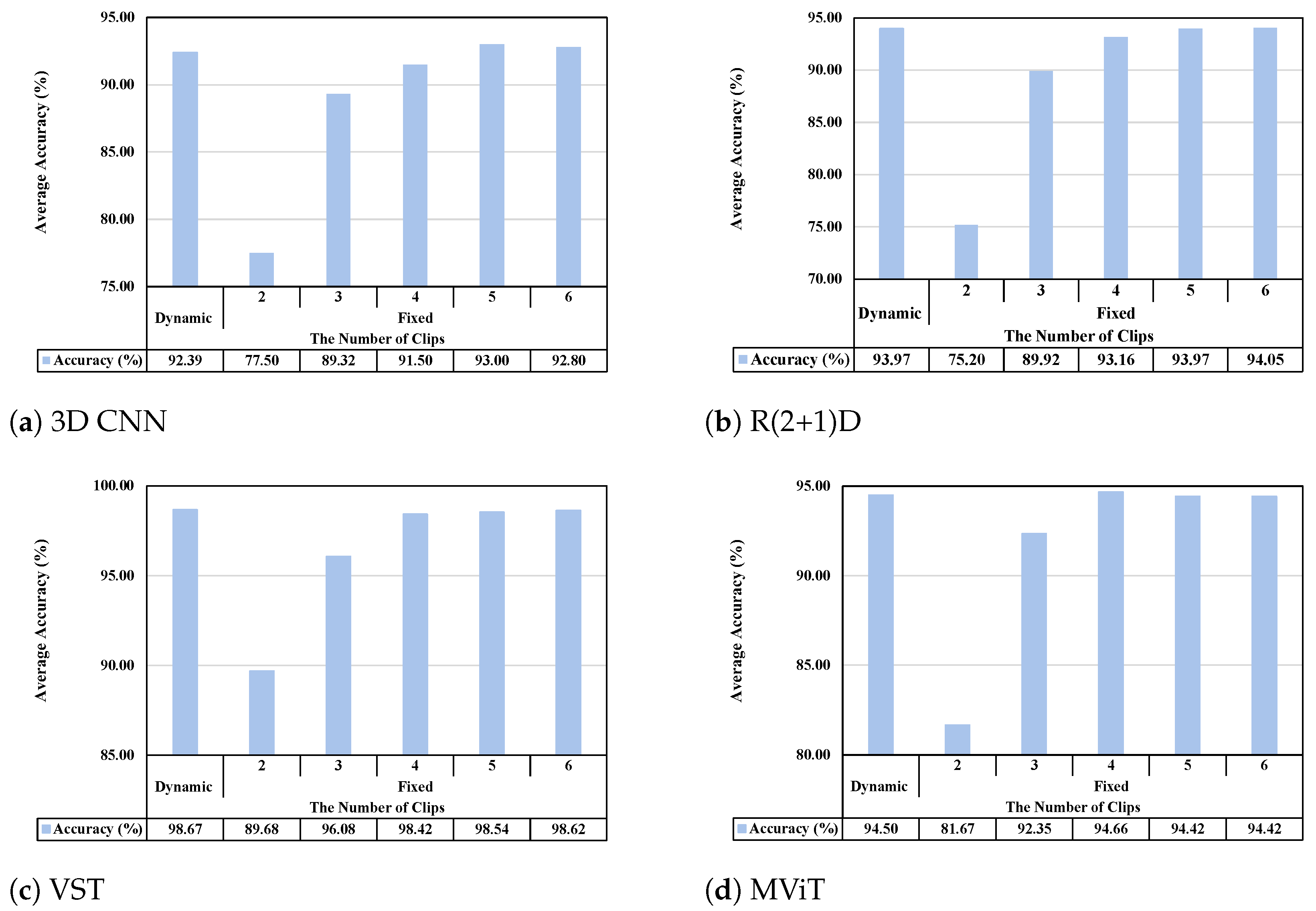
Figure 5 compares the average accuracy between the dynamic and fixed methods across different models. Figure 6 presents the comparison of average inference time between the dynamic and fixed methods across different models. As shown in Figure 5 and Figure 6, for 3D CNNs, the fixed method achieved the highest accuracy at 93.00%, with an inference time of 0.24 s using 5 clips, whereas the dynamic method had a slightly lower accuracy of 92.39%, but improved the inference time to 0.21 s, representing a 12.50% reduction. In R(2+1)D, the fixed method reached a 94.05% accuracy with an inference time of 0.054 s using 6 clips, while the dynamic method achieved a 93.97% accuracy but significantly reduced the inference time to 0.039 s—a 27.78% decrease. For VSTs, when using 6 clips, the fixed method achieved its best performance with 98.62% accuracy and an inference time of 0.49 s. However, the dynamic method not only slightly outperformed it with a 98.67% accuracy but also significantly reduced the inference time to 0.35 s, representing a 28.57% improvement. Lastly, for MViTs, the fixed method achieved its best performance with 4 clips, reaching a 94.66% accuracy and an inference time of 0.14 s. The dynamic method resulted in a slightly lower accuracy of 94.50% with the same inference time, indicating that the dynamic method did not provide any advantage in terms of inference time in this case.

When the number of clips is 2, we observe that the accuracy for all models (MViTs, 3D CNNs, R(2+1)D, and VSTs) is at its lowest. This indicates that, with only two clips, the generated clips do not adequately capture the temporal context of the video, resulting in a noticeable decrease in performance. In contrast, when the coverage value exceeds 1, the entire temporal information of the video will have already been used at least once. In the experiment, when the coverage value is greater than 1, the number of generated clips was 4 or more. Beyond this point, further increasing the number of clips does not lead to significant accuracy improvements. In some cases, excessive clip generation may potentially lead to minor accuracy degradation, as observed in our experiments with 3D CNNs, which showed lower accuracy with 6 clips compared to 5 clips, and MViTs, which demonstrated decreased performance with 5 clips compared to 4 clips. In other words, generating too many clips for recognition may not provide any benefit in terms of recognition accuracy and inference efficiency.

When comparing average inference times across different models, our results demonstrate significant computational efficiency gains with the dynamic method.

Table 11. Comparison of dynamic and fixed clip generation efficiency.

Model	Average Number of Clips		Inference Time (s)		Inference Time Reduction Rate (%)	Clip Reduction Rate (%)
	Fixed	Dynamic	Fixed	Dynamic
3D CNN	5	4.37	0.24	0.21	12.50	12.60
R(2+1)D	6	4.22	0.054	0.039	27.78	29.67
VST	6	4.22	0.49	0.35	28.57	29.67
MViT	4	4.37	0.14	0.14	0.00	−9.25

presents a comparison between the dynamic method and the fixed method, which achieved the highest accuracy for each model. The table highlights key metrics, including the average number of clips generated, inference time (in seconds), inference time reduction rate, and clip reduction rate for each model.

It is important to note that although the number of clips is dynamically adjusted depending on the length of the video, each clip still contains a fixed number of frames (e.g., 16 or 30). As a result, shorter videos generate fewer clips, reducing the total number of frames passed through the model and effectively decreasing inference time.

For 3D CNNs, the dynamic method achieves a 12.50% reduction in inference time, with an average inference time of 0.21 s compared to 0.24 s for the fixed method. This reduction is accompanied by a slight decrease in the number of clips, with the dynamic method generating an average of 4.37 clips, compared to 5 clips for the fixed method. This suggests that by dynamically adjusting the number of clips based on video content, the dynamic method offers a more computationally efficient solution without significantly compromising accuracy.

Similarly, R(2+1)D shows a notable 27.78% reduction in inference time, decreasing from 0.054 s for the fixed method to 0.039 s for the dynamic method. In this case, the dynamic method generates slightly fewer clips (4.22 clips) compared to the fixed method (6 clips), demonstrating the method’s efficiency in optimizing clip generation without sacrificing performance.

For VSTs, the dynamic method achieves a 28.57% reduction in inference time, from 0.49 s for the fixed method to 0.35 s with dynamic clip generation. The number of clips generated in the dynamic approach (4.22 clips) is slightly lower than in the fixed approach (6 clips), further improving computational efficiency while maintaining high accuracy.

However, for MViTs, both the fixed and dynamic methods result in the same inference time of 0.14 s. The number of clips generated by both methods remains the same (4.37 clips for the dynamic method and 4 clips for the fixed method), but the dynamic method’s clip reduction rate is negative (−9.25%), suggesting that the dynamic method does not provide the same level of improvement for MViTs as it does for other models.

In summary, the dynamic clip generation method significantly reduces inference times for three out of the four models (3D CNNs, R(2+1)D, and VSTs), while also reducing the number of clips needed for video recognition. These results demonstrate that the dynamic method offers a substantial computational efficiency advantage in sign language recognition tasks, especially for models that benefit from flexible clip generation.

Overall, our results demonstrate that the dynamic clip generation method based on our proposed coverage metric delivers significant advantages across multiple models. Particularly impressive results were observed with R(2+1)D and VST, where we achieved inference time reductions of 27.78% and 28.57% respectively, while maintaining or even improving accuracy. By adjusting the number of clips according to each video’s temporal complexity, this method prevents computational waste while ensuring sufficient information capture. Our approach is particularly valuable for real-time video recognition applications where processing speed is critical without compromising recognition performance.

5. Conclusions

Sign language recognition (SLR) services have become increasingly important in recent years, driven by the growing need for inclusive communication in both public and private sectors. As advancements in deep learning and computer vision continue, efficient and accurate SLR systems are vital for enabling real-time communication, especially in resource-constrained environments.

In this study, we proposed a dynamic clip generation method to enhance the efficiency and accuracy of sign language recognition (SLR). By adaptively adjusting the number of clips based on our proposed coverage metric, our method overcomes the limitations of traditional fixed clip generation methods, which use a predetermined number of clips regardless of video length. Unlike these conventional method, our dynamic method ensures that longer videos retain sufficient contextual information while preventing redundant processing in shorter videos. This optimal balance between computational efficiency and recognition accuracy makes our method particularly valuable for real-time SLR applications, especially in resource-constrained environments.

Experimental results across multiple model architectures demonstrated that the optimal number of clips varied by model: 5 clips for 3D CNNs, 6 clips for the R(2+1)D and Video Swin Transformer (VST), and 4 clips for Multiscale Vision Transformers (MViTs). Our dynamic method successfully reduced inference time while maintaining or even improving accuracy compared to fixed methods. Specifically, we achieved inference time reductions of 12.50% for 3D CNNs, 27.78% for R(2+1)D, and 28.57% for VSTs, with accuracy remaining within a 0.5% margin or better than the fixed method. Notably, VSTs saw a 28.57% reduction in inference time, with the dynamic method slightly outperforming the fixed method in accuracy (98.67% vs. 98.62%). For MViTs, both methods showed similar performance, suggesting that the effectiveness of dynamic clip generation may depend on the model’s architecture and temporal processing capabilities.

Our analysis revealed that when the coverage value fell below 1.0, recognition accuracy declined significantly due to insufficient contextual information, confirming the importance of our coverage metric as a reliable indicator for clip generation decisions. Additionally, we observed that excessive clip generation (coverage values significantly above 1.0) sometimes led to redundancy, negatively impacting both computational efficiency and recognition accuracy, as seen in the performance degradation of 3D CNNs and MViTs with higher clip counts.

In conclusion, this work represents an important step toward more efficient and accurate sign language recognition systems that can operate effectively across different computational platforms. By dynamically adjusting clip generation based on contextual requirements, our method offers significant improvements in both inference time and accuracy, contributing to the development of more robust and scalable SLR systems.