Passive Earth Pressure and Soil Arch Shape: A Two-Dimensional Analysis

Abstract

This paper introduces an analytical method for passive earth pressure calculation based on a rigorous stress field analysis within the sliding wedge. Unlike traditional horizontal layer methods, this approach directly solves for the stress state at any point within the wedge by analyzing the equilibrium of 2D differential soil elements under appropriate boundary conditions, eliminating the need for a priori assumptions about the soil arch shape. The method yields the passive earth pressure distribution on the retaining structure and derives the soil arch shape analytically from major principal stress trajectories. This derived arch shape differs notably from conventional circular or parabolic assumptions, especially at higher soil–wall friction angles. Parametric studies show that the passive earth pressure coefficient increases with internal friction angle and surcharge. However, a key finding is the non-monotonic dependence of the passive earth pressure coefficient on the soil–wall friction angle, contrasting with many existing theories. Comparisons show predictions by the proposed method align well with experimental data, particularly offering a better representation of pressure distributions in the lower regions of retaining walls compared to Coulomb theory and other existing methods.

1. Introduction

The issue of earth pressure on retaining walls is one of the core research topics in geotechnical engineering, with significant implications for the design optimization and stability assessment of retaining structures. While the classical Coulomb, Rankine, and Caquot theories [1] are widely applied in practice due to their simplicity and computational efficiency, their assumption of linear earth pressure distribution conflicts with the nonlinear patterns observed in field measurements and model tests [2,3]. This discrepancy has prompted extensive theoretical studies on nonlinear earth pressure distributions, primarily through the application of limit equilibrium methods and limit analysis approaches.

The majority of earth-retaining structures are primarily subjected to active earth pressure, leading to extensive research on active earth pressure theory by scholars worldwide. Following the introduction of a nonlinear earth pressure calculation method based on horizontal layer analysis, this approach has been systematically refined and extended to analyze active earth pressure under complex conditions [4,5]. Moreover, substantial experimental evidence has demonstrated the ubiquity of soil arching effects within soil masses. Handy [6] attributed the nonlinear distribution of earth pressure to soil arching, characterizing the arch shape as the minor principal stress trajectory, and subsequently developed a curved distribution calculation for active earth pressure by integrating this concept with horizontal layer analysis. Thereafter, calculation methods that integrate the horizontal layer analysis with soil arching effects have gained increasing traction among scholars, yielding substantial advancements. For instance, Liu et al. [7] derived analytical solutions for the lateral earth pressure coefficient and active earth pressure under seismic conditions, considering both soil arching and vertical cracks within the framework of the unified strength theory under plane strain conditions. To better represent soil failure mechanisms and improve computational accuracy, analytical solutions incorporating curved sliding surfaces have been developed for active earth pressure, addressing sliding surface morphology [8,9]. Additionally, limit analysis methods, which served as an alternative approach, have also been effectively employed to study active earth pressure under complex conditions. Wang et al. [10], based on limit analysis theory, introduced the concept of critical width to distinguish between finite-width and semi-infinite soil masses in scenarios like retaining walls near rock or existing structures, and formulated computational equations for active earth pressure in finite soil masses, providing a theoretical foundation for relevant engineering designs.

Compared to the extensively studied problem of active earth pressure, theoretical investigations on passive earth pressure remain relatively limited. Nevertheless, passive earth pressure plays a critical role in the safety and stability of various geotechnical structures, such as excavation support systems, bridge pier foundations, retaining walls, and pile cap foundations. Therefore, a thorough theoretical understanding of passive earth pressure is of significant importance for both design optimization and reliable performance in engineering practice.

The horizontal layer method (see Figure 1a), combined with major principal stress trajectories, is also widely employed to investigate the distribution patterns of passive earth pressure [11,12,13]. Variations in existing studies primarily stem from differing assumptions regarding the shape of the sliding surface and the soil arch (trajectory of the major principal stress). These assumptions directly impact the calculated magnitude and distribution characteristics of passive earth pressure. Extending this approach, researchers have adapted it to complex conditions, including cohesive and multilayered backfill, seismic loading, seepage, and narrow excavations [14,15,16,17]. In practical applications, achieving a fully mobilized passive state requires wall displacement, yet, in most cases, movement is insufficient, resulting in earth pressure values between at-rest and passive states. To address this, studies have explored non-limit state passive earth pressure, incorporating displacement effects for more accurate predictions [18,19]. Meanwhile, limit analysis has also gained traction. For instance, Li [20] derived the magnitude of passive earth pressure under seismic action using the upper-bound analysis, further exploring the effects of factors like backfill height and internal friction angle on wall stability.

Significant progress has been achieved in calculating passive earth pressure using the horizontal layer method coupled with the soil arching effect, enabling reasonable descriptions of its distribution patterns to some extent. However, several limitations persist: (1) no consensus exists on soil arching shape (major principal stress trajectory) under passive limit equilibrium, with conflicting convex and concave assumptions that often misalign with observed behavior; (2) the assumption that all points in the sliding wedge are at limit equilibrium contradicts observations; (3) shear stress induced by principal stress rotation is often overlooked, leading to discrepancies in predicted earth pressure distribution.

To address these limitations and improve the estimation of passive earth pressure, this study adopts a two-dimensional differential element approach. An arbitrary element dxdz within the sliding wedge is selected as the basic unit for analysis (see Figure 1b). This approach avoids the assumption of soil arching shapes and accounts for the effects of shear stresses. By solving the equilibrium differential equations under reasonable assumptions and boundary conditions, analytical stress solutions are derived for any point within the wedge. Based on these solutions, the magnitude, distribution, and point of application of passive earth pressure on the retaining wall are determined. Furthermore, the trajectory of the major principal stress is derived analytically and compared with the assumed trajectories adopted in previous studies. Finally, parametric analyses are carried out to explore the influence of key factors on passive earth pressure, and comparisons with theoretical and experimental results confirm the accuracy and applicability of the proposed approach.

2. Derivation of Equilibrium Differential Equations and Solution for Passive Earth Pressure

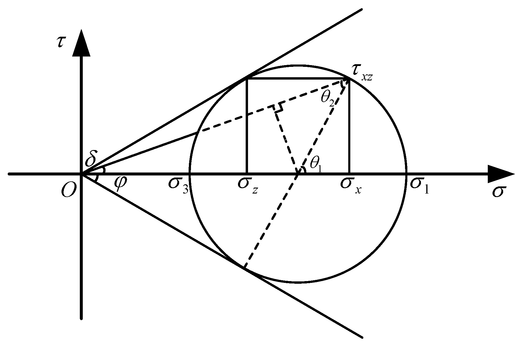
2.1. Establishment of Equilibrium Differential Equations

The problem of passive earth pressure acting on a retaining wall is analyzed under the following assumptions: (1) The problem is idealized as a two-dimensional plane strain condition. (2) The backfill material is a homogeneous, isotropic sand (cohesionless). (3) The shear strength behavior of the backfill adheres to the Mohr–Coulomb failure criterion. (4) The retaining wall is vertical, with a rough back surface (mobilizing friction), and the backfill surface is horizontal. (5) The potential sliding surface within the backfill is assumed to be a plane originating from the wall heel.

Figure 1b illustrates the potential sliding plane and stress conditions of an arbitrary differential element (dxdz) within the soil mass when the passive state is achieved. A Cartesian coordinate system (x, z) is established with its origin at the wall heel, where z is positive upwards. Considering the differential element located at coordinates (x, z) within the sliding soil mass, its stress state is shown in Figure 1b. Based on continuum mechanics principles, the equilibrium equations are established as follows:

$${\displaystyle \frac{\partial {\sigma }_x}{\partial x}}-{\displaystyle \frac{\partial {\tau }_{zx}}{\partial z}}=0,$$

(1)

$${\displaystyle \frac{\partial {\sigma }_z}{\partial z}}-{\displaystyle \frac{\partial {\tau }_{xz}}{\partial x}}=-\gamma ,$$

(2)

where ${\sigma }_x$ is the horizontal normal stress, ${\sigma }_z$ is the vertical normal stress, ${\tau }_{zx}$ and ${\tau }_{xz}$ are the shear stress, and $\gamma$ is the unit weight of the soil. Compressive normal stress is adopted as positive in this paper.

2.2. Boundary Conditions

(1)

Upper Surface (z = H):

The backfill surface is horizontal and subjected to a uniform load q. Thus, at z = H, ${\sigma }_z=q$, ${\tau }_{zx}=0$.

(2)

Soil–Wall Interface (x = 0):

At the soil–wall interface (x = 0), the soil element reaches a state of limit equilibrium, with the soil–wall friction angle (external friction angle) $\delta$ fully mobilized. The stress state, represented by a Mohr’s circle in Figure 2, yields the following relationships:

$${\tau }_{\mathrm{w}}(z)={\mu }_{\mathrm{w}}{\sigma }_{wx}(z);$$

(3)

$${\sigma }_{wx}(z)=K_{\mathrm{wp}}{\sigma }_{wz}(z).$$

(4)

where ${\tau }_{\mathrm{w}}$, ${\sigma }_{wx}$, and ${\sigma }_{wz}$ represent the shear stress, horizontal normal stress, and vertical normal stress, respectively, acting on the soil element adjacent to the wall face; ${\mu }_{\mathrm{w}}$ is the external friction coefficient, defined as ${\mu }_{\mathrm{w}}=\tan \delta$; and $K_{\mathrm{wp}}$ (distinct from the passive earth pressure coefficient $K_p$) is the lateral stress ratio at the wall. From Figure 2, the geometric relationships are as follows:

$${\theta }_1={\theta }_2+\delta , \sin {\theta }_2=\sin \delta /\sin \phi .$$

(5)

Thus,

$${\theta }_1=\delta +{\sin }^{-1}(\sin \delta /\sin \phi ),$$

(6)

and we can obtain the following:

$$K_{\mathrm{wp}}={\displaystyle \frac{1+\cos (\mathrm{s}\mathrm{i}{\mathrm{n}}^{-1}(\mathrm{s}\mathrm{i}\mathrm{n}\delta /\mathrm{s}\mathrm{i}\mathrm{n}\phi )+\delta )\mathrm{s}\mathrm{i}\mathrm{n}\phi }{1-\cos (\mathrm{s}\mathrm{i}{\mathrm{n}}^{-1}(\mathrm{s}\mathrm{i}\mathrm{n}\delta /\mathrm{s}\mathrm{i}\mathrm{n}\phi )+\delta )\mathrm{s}\mathrm{i}\mathrm{n}\phi .}}$$

(7)

Substituting Equation (4) into Equation (3), the stress boundary condition at x = 0 becomes the following:

$${\tau }_{\mathrm{w}}(z)=A_{\mathrm{p}}{\sigma }_{\mathrm{wz}}(z),$$

(8)

where $A_{\mathrm{p}}={\mu }_{\mathrm{w}}{K}_{\mathrm{wp}}$.

(3)

Potential Sliding Surface ($x=z\cot \varphi$):

The classical limit equilibrium method developed by Coulomb assumes a planar sliding surface for passive earth pressure behind retaining walls, with its inclination angle $\varphi$ determined by the internal friction angle $\phi$ and the wall friction angle $\delta$. However, this analysis neglected the soil arching effect. Subsequent studies attempted to incorporate soil arching by considering the equilibrium of horizontal soil layers [11,12,13]. While advancing the analysis, these methods often relied on the simplifying assumption of zero shear stress acting on horizontal layers, which may not accurately represent actual soil behavior in the field.

On the other hand, research has shown that, under passive conditions, the inclination of the sliding surface is affected to some extent by soil–wall friction angle but is mainly governed by the internal friction angle. Furthermore, it has been suggested that variations in the specific shape and inclination angle of the sliding surface tend to have a relatively minor impact on the magnitude of the calculated earth pressure [21]. Based on these findings, several researchers, including Sahoo and Ganesh [22] and Dalvi and Pise [23], assumed that the inclination of the sliding surface depends only on the internal friction angle. By combining this assumption with the equilibrium of horizontal soil layers and incorporating soil arching effects, their analyses yielded passive earth pressure values that were reported to align well with experimental data.

For the sake of analytical simplicity and ease of calculation, this study adopts the assumption proposed in References [22,23], where the inclination of the potential sliding surface with respect to the horizontal is considered a function of the internal friction angle only (i.e., $\varphi =\pi /4-\phi /2$). Under the Mohr–Coulomb criterion, this assumption implies that the principal stress directions remain unchanged along the sliding plane.

2.3. Solution of the Equilibrium Equations

The traditional horizontal layer method assumes that a uniform average vertical stress acts across the entire soil layer at a given depth. To further account for soil arching effects within this framework, later studies generally introduced additional assumptions. Specifically, it is commonly assumed that, at the same depth, the magnitudes of the principal stresses remain constant while their orientations vary, and that all soil elements are in a state of limit equilibrium. Nonetheless, the soil experiences intricate stress–strain evolutions throughout its interaction with the retaining wall as it approaches the limit equilibrium state, which makes it challenging to strictly fulfill these assumptions.

An alternative, influential simplification originates from Janssen’s [24] foundational analysis of silo pressures, wherein the vertical normal stress ${\sigma }_z$ is assumed to remain constant along any horizontal plane (i.e., $\partial {\sigma }_z/\partial x=0$). While this is an idealization, its effectiveness for analyzing granular media has been supported by multiple lines of evidence: (i) its successful application in silo pressure and arching theories [25,26]; (ii) numerical simulations of retaining wall problems reveal only minor horizontal variations in ${\sigma }_z$ [21]; (iii) its incorporation into analytical derivations of active earth pressure has yielded results consistent with experimental observations [9].

Considering this theoretical development and supporting evidence, the present analysis of passive earth pressure adopts Janssen’s assumption, positing that the vertical normal stress ${\sigma }_z$ is invariant with the horizontal coordinate x at any given depth z. Applying this condition to the vertical equilibrium equation employed in this study (Equation (2)), and subsequently differentiating with respect to x, leads to the following:

$${\displaystyle \frac{{\partial }^2{\tau }_{xz}}{\partial x^2}}=0.$$

(9)

The general solution to Equation (9) indicates a linear distribution of shear stress with x as follows:

$${\tau }_{xz}(x,z)=C_1(z)x+C_2(z),$$

(10)

where $C_1(z)$ and $C_2(z)$ are integration constants determined by boundary conditions. Applying boundary conditions—specifically, at x = 0, ${\tau }_{\mathrm{w}}(z)=A_{\mathrm{p}}{\sigma }_{\mathrm{wz}}(z)$; and at $x=z\cot \varphi$, ${\tau }_{zx}(z,x)=0$—yields the specific expression for the shear stress:

$${\tau }_{zx}(z,x)=(A_{\mathrm{p}}-{\displaystyle \frac{A_{\mathrm{p}}}{z\cot \varphi }}x){\sigma }_{\mathrm{wz}}(z)=(A_{\mathrm{p}}-m_{\mathrm{p}}{\displaystyle \frac{x}{z}}){\sigma }_z(z),$$

(11)

where $m_{\mathrm{p}}=A_{\mathrm{p}}\tan \varphi$.

Substituting this expression for shear stress (Equation (11)) into the vertical equilibrium equation (Equation (2)) results in a first-order linear non-homogeneous ordinary differential equation governing the vertical stress ${\sigma }_z$:

$${\displaystyle \frac{\partial {\sigma }_z}{\partial z}}+m_{\mathrm{p}}{\displaystyle \frac{{\sigma }_z}{z}}=-\gamma .$$

(12)

The general solution to Equation (12) takes the following form:

$${\sigma }_z(z)=\left\{\begin{array}{l}{C}_{3}z-\gamma z\ln (z)\hspace{0.33em}\hspace{0.33em}\hspace{0.33em}\hspace{0.33em}\hspace{0.33em}\hspace{0.33em}\hspace{0.33em}\hspace{0.33em}\hspace{0.33em}\hspace{0.33em}\hspace{0.33em}\hspace{0.33em}{m}_{\mathrm{p}}=-1\\ C_4{z}^{-m_{\mathrm{p}}}-{\displaystyle \frac{\gamma z}{m_{\mathrm{p}}+1}}\hspace{0.33em}\hspace{0.33em}\hspace{0.33em}\hspace{0.33em}\hspace{0.33em}\hspace{0.33em}\hspace{0.33em}\hspace{0.33em}\hspace{0.33em}\hspace{0.33em}\hspace{0.33em}{m}_{\mathrm{p}}\ne -1\end{array}\right.,$$

(13)

where $C_3$ and $C_4$ are integration constants determined by the boundary conditions. Given that $m_{\mathrm{p}}=A_{\mathrm{p}}\tan \varphi \ge 0$ under considered conditions, the case $m_{\mathrm{p}}=-1$ is excluded. By applying the upper boundary condition ${\sigma }_z=q$ at $z=H$ to the second case, the constant $C_4$ can be determined, leading to the explicit solution for the vertical stress as follows:

$${\sigma }_z(z)={\displaystyle \frac{\gamma H}{1+m_{\mathrm{p}}}}\left[{\left({\displaystyle \frac{z}{H}}\right)}^{-m_{\mathrm{p}}}-{\displaystyle \frac{z}{H}}\right]+q{\left({\displaystyle \frac{z}{H}}\right)}^{-m_{\mathrm{p}}}.$$

(14)

Substituting this solution (Equation (14)) back into the expression for shear stress (Equation (11)), the shear stress at any point within the wedge is obtained as follows:

$${\tau }_{zx}(x,z)=\left(A_{\mathrm{p}}-m_{\mathrm{p}}{\displaystyle \frac{x}{z}}\right)\left\{{\displaystyle \frac{\gamma H}{1+m_{\mathrm{p}}}}\left[{\left({\displaystyle \frac{z}{H}}\right)}^{-m_{\mathrm{p}}}-{\displaystyle \frac{z}{H}}\right]+q{\left({\displaystyle \frac{z}{H}}\right)}^{-m_{\mathrm{p}}}\right\}.$$

(15)

Finally, substituting the shear stress distribution (Equation (15)) into the horizontal equilibrium equation (Equation (1)) and integrating with respect to x yields the horizontal stress ${\sigma }_x$:

$${\sigma }_x(x,z)=\left[K_{\mathrm{wp}}-A_{\mathrm{p}}{m}_{\mathrm{p}}{\displaystyle \frac{x}{z}}+{\displaystyle \frac{m_{\mathrm{p}}(m_{\mathrm{p}}+1)}{2}}{\left({\displaystyle \frac{x}{z}}\right)}^2\right]{\sigma }_z(z)-A_{\mathrm{p}}\gamma x+{\displaystyle \frac{m_{\mathrm{p}}\gamma x^2}{2z}}.$$

(16)

As can be seen from Equation (16), the stress theoretically tends to infinity as z = 0. In practical applications, this singularity can be avoided by slightly extending the wall height (e.g., by 1% of H) so that the corner region is modeled as a finite-width soil element rather than a sharp geometric point.

In summary, Equations (14)–(16) provide the complete analytical solution for the stress field at any point (x, z) within the soil wedge.

2.4. Calculation of Passive Earth Pressure

The intensity of the horizontal component of passive earth pressure acting on the wall face at depth z, denoted ${\sigma }_{\mathrm{wx}}$, is obtained by setting x = 0 in Equation (16):

$${\sigma }_{\mathrm{wx}}(z)={\displaystyle \frac{K_{\mathrm{wp}}\gamma H}{1+m_{\mathrm{p}}}}\left[{\left({\displaystyle \frac{z}{H}}\right)}^{-m_{\mathrm{p}}}-{\displaystyle \frac{z}{H}}\right]+K_{\mathrm{wp}}q{\left({\displaystyle \frac{z}{H}}\right)}^{-m_{\mathrm{p}}}.$$

(17)

The resultant horizontal passive force $P_{\mathrm{ph}}$ acting on a wall of height H is obtained by integrating the pressure intensity over the depth of the wall. When $\hspace{0.33em}0<m_{\mathrm{p}}<1$, the integration yields the following:

$$P_{\mathrm{ph}}={\displaystyle {\int }_0^H{\sigma }_{\mathrm{wx}}(z)\mathrm{d}z}={\displaystyle \frac{K_{\mathrm{wp}}\gamma H^2}{1-m_{\mathrm{p}}}}({\displaystyle \frac{1}{2}}+{\displaystyle \frac{q}{\gamma H}})$$

(18)

It is noted that, if $m_{\mathrm{p}}\ge 1$, the integral in Equation (18) diverges, suggesting an infinite horizontal force, which is physically unrealistic. However, as illustrated in Figure 3, contour plots of $m_{\mathrm{p}}$ indicate that $m_{\mathrm{p}}$ typically reaches a maximum value of approximately 0.5 under the condition $\delta \le \phi$. Therefore, the condition $m_{\mathrm{p}}\ge 1$ is not encountered, ensuring that Equation (18) yields a finite resultant horizontal force within this theoretical framework.

The resultant vertical force acting on the wall is the integral of the shear stress ${\tau }_{\mathrm{w}}$ along the wall height:

$$P_{\mathrm{pv}}={\displaystyle {\int }_0^H{\tau }_{\mathrm{w}}(z)\mathrm{d}z}=P_{\mathrm{ph}}\tan \delta .$$

(19)

The total resultant passive earth force is then given by the following:

$$P_{\mathrm{p}}=\sqrt{P_{\mathrm{ph}}^2+P_{\mathrm{pv}}^2}={\displaystyle \frac{P_{\mathrm{ph}}}{\cos \delta }}.$$

(20)

The moment exerted by the horizontal earth pressure about the bottom of the wall (z = 0) is calculated as follows:

$$M_{\mathrm{p}}={\displaystyle {\int }_0^H{\sigma }_{\mathrm{wx}}(z)z\mathrm{d}z}={\displaystyle \frac{K_{\mathrm{wp}}\gamma H^3}{2-m}}({\displaystyle \frac{1}{3}}+{\displaystyle \frac{q}{\gamma H}}),$$

(21)

and the height of application $h_{\mathrm{p}}$ of the horizontal resultant force is then given by the following:

$$h_{\mathrm{p}}={\displaystyle \frac{M_{\mathrm{p}}}{P_{\mathrm{ph}}}}={\displaystyle \frac{2}{3}}{\displaystyle \frac{1-m_{\mathrm{p}}}{2-m_{\mathrm{p}}}}{\displaystyle \frac{\gamma H+3q}{\gamma H+2q}}H.$$

(22)

Finally, the passive earth pressure coefficient, defined as $K_{\mathrm{p}}=2P_{\mathrm{p}}/\gamma H^2$, can be derived as follows:

$$K_{\mathrm{p}}={\displaystyle \frac{K_{\mathrm{wp}}}{(1-m_{\mathrm{p}})cos\delta }}(1+{\displaystyle \frac{2q}{\gamma H}}).$$

(23)

Figure 4a–d illustrates the distributions of normalized vertical stress, shear stress, horizontal stress, and the relative principal stress ratio within the soil wedge. These results were obtained using the following parameters: internal friction angle $\phi =20°$, soil–wall friction angle $\delta =0.2\phi$, and applied surcharge $q=0.5\gamma H$ (with wall height H = 1 m assumed for scaling). The term $K_{\mathrm{pr}}$ in Figure 4d represents the Rankine passive earth pressure coefficient, defined as $K_{\mathrm{pr}}={\tan }^2(\pi /4+\phi /2)$.

Analysis of these distributions (Figure 4) reveals the following: (1) The vertical normal stress shows a clear layered distribution and increases nonlinearly with depth. In particular, within the middle and lower regions of the wedge, the vertical stress significantly exceeds the nominal overburden pressure $(\gamma z+q)$. This phenomenon is attributed to the soil arching effect, in which the frictional resistance along the wall back and the sliding surface restricts vertical displacement, leading to stress redistribution and concentration. (2) The shear stress ${\tau }_{zx}$ is observed to decrease progressively with increasing horizontal distance x from the wall. However, its variation with vertical depth z appears non-monotonic, generally increasing initially before subsequently decreasing. (3) The horizontal normal stress ${\sigma }_x$ exhibits a continuous increase with depth z at any given x. Conversely, along a horizontal plane (constant z), ${\sigma }_x$ varies non-monotonically with horizontal distance. (4) The relative stress ratio approaches unity in localized zones, specifically adjacent to the wall face and along the middle-to-lower portion of the sliding surface. This signifies that soil within these regions has attained the limit equilibrium state, while the soil in other areas has not yet reached this critical condition.

3. Analysis of Soil Arching Under Passive Conditions

In passive earth pressure analysis, the soil arch shape is commonly defined by the trajectory of the major principal stress. The horizontal layer method incorporating soil arching effects often assumes this trajectory to follow circular, parabolic, or catenary forms. In contrast, the present study does not impose a predefined shape. Instead, the trajectory of the major principal stress is derived directly from the computed stress field within the sliding wedge. The resulting curve is then compared with commonly assumed circular and parabolic arch shapes.

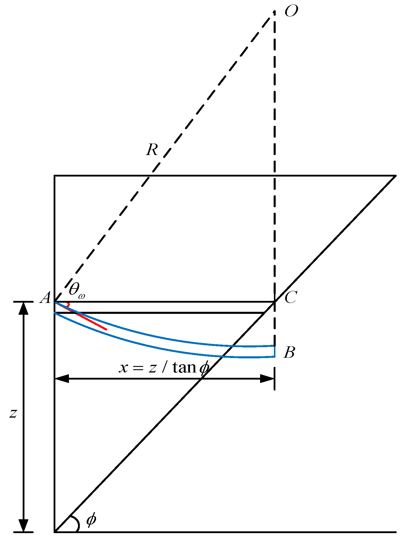
3.1. Derivation of Soil Arch Shape

Stress analysis within the wedge-shaped backfill reveals that the major principal stress varies in magnitude and direction at a given height. This observation stands in contrast to the assumptions commonly adopted in horizontal layer methods incorporating soil arching effects, which typically assume that the magnitude of the major principal stress remains constant along each horizontal layer, with only its orientation changing.

The stress state of an arbitrary soil element along the soil arch is illustrated in Figure 5. The slope of the tangent to the soil arch curve is determined to be the tangent of the angle between the major principal stress direction and the horizontal axis, expressed as $-\tan {\xi }_{\tau }\prime$. The negative sign indicates that the arch exhibits a downward concave profile. The relationship depicted in Figure 5 is given by the following:

$$\tan 2{\xi }_{\tau }\prime ={\displaystyle \frac{2{\tau }_{zx}}{{\sigma }_x-{\sigma }_z}},$$

(24)

where ${\xi }_{\tau }\prime$ denotes the angle between the major principal stress direction and the horizontal.

From this, we can obtain the following:

$$\tan {\xi }_{\tau }\prime =\left\{\begin{array}{l}{\displaystyle \frac{-1+\sqrt{{\tan }^{2}2{\xi }_{\tau }\prime +1}}{\tan 2{\xi }_{\tau }\prime }}\hspace{0.33em}\hspace{0.33em}\hspace{0.33em}\hspace{0.33em}\hspace{0.33em}\hspace{0.33em}\hspace{0.33em}\hspace{0.33em}\hspace{0.33em}\tan 2{\xi }_{\tau }\prime \ge 0\\ {\displaystyle \frac{-1-\sqrt{{\tan }^{2}2{\xi }_{\tau }\prime +1}}{\tan 2{\xi }_{\tau }\prime }}\hspace{0.33em}\hspace{0.33em}\hspace{0.33em}\hspace{0.33em}\hspace{0.33em}\hspace{0.33em}\hspace{0.33em}\hspace{0.33em}\hspace{0.33em}\tan 2{\xi }_{\tau }\prime <0\end{array}\right..$$

(25)

Substitution of Equation (24) into Equation (25) yields the following:

$$\tan {\xi }_{\tau }\prime (\sigma )=\left\{\begin{array}{l}{\displaystyle \frac{-1+\sqrt{{(\frac{2{\tau }_{zx}}{{\sigma }_x-{\sigma }_z})}^2+1}}{\frac{2{\tau }_{zx}}{{\sigma }_x-{\sigma }_z}}}\hspace{0.33em}\hspace{0.33em}\hspace{0.33em}\hspace{0.33em}{\sigma }_x\ge {\sigma }_z\\ {\displaystyle \frac{-1-\sqrt{{(\frac{2{\tau }_{zx}}{{\sigma }_x-{\sigma }_z})}^2+1}}{\frac{2{\tau }_{zx}}{{\sigma }_x-{\sigma }_z}}}\hspace{0.33em}\hspace{0.33em}\hspace{0.33em}\hspace{0.33em}{\sigma }_x<{\sigma }_z\end{array}\right.,$$

(26)

The expression of the soil arch curve, denoted as $f_{\mathrm{arch}}(x)$, is obtained by integrating the tangent slope $-\tan {\xi }_{\tau }\prime$ with respect to x, given by the following:

$$f_{\mathrm{arch}}(x,z)=-{\displaystyle {\int }_0^x\tan {\xi }_{\tau }\prime (t,z)dt}+z.$$

(27)

Equation (27) provides the expression for the soil arch curve at a given height z. By substituting the stress solutions (Equations (14)–(16)) into Equation (27) and performing the integration, an explicit expression for the soil arch curve is obtained. For the passive sliding wedge considered in this study, the range of x is defined as (0, $z\cot \varphi$).

The distribution of the soil arch within the backfill is shown in Figure 6 for $\phi =30°$ $q=0.5\gamma H$, under varying soil–wall friction angles ($\delta =0.3\phi$ in Figure 6a, $\delta =0.5\phi$ in Figure 6b). The major and minor principal stress directions are indicated by dark green and red lines, respectively. The results show that soil arch curves at different depths exhibit similar shapes. The slopes of the arches at different heights are nearly constant at the wall face (x = 0) and gradually decrease with increasing horizontal distance, eventually approaching zero at the sliding surface. This trend is consistent with the initial assumption of no principal stress rotation along the sliding boundary. Additionally, increasing the soil–wall friction angle leads to steeper arch profiles, reflecting a more pronounced soil arching effect within the backfill.

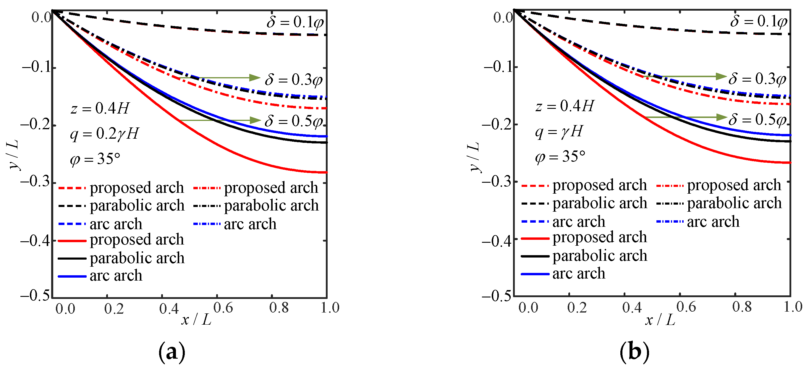
3.2. Comparison with Circular and Parabolic Arches

Expressions for circular (arc) and parabolic arches under the same sliding surface are derived for comparative analysis.

(1)

Circular Arch

In horizontal layer methods that incorporate soil arching effects, the sliding backfill is assumed to be in a limit equilibrium state at every point. Based on the stress conditions at the wall (see Figure 2), the angle ${\theta }_{\mathrm{w}}$ between the major principal stress and the horizontal direction can be determined as follows:

$${\theta }_{\mathrm{w}}=({\sin }^{-1}(\sin \delta /\sin \phi )+\delta )/2.$$

(28)

According to the Mohr–Coulomb failure criterion, at limit equilibrium, the angle between the major principal stress direction and the failure plane is $\pi /4-\phi /2$. Consequently, at the sliding surface itself, the major principal stress experiences no rotation, as shown in Figure 7. The circular arch geometry in Figure 7 satisfies the following:

$$R\sin {\theta }_{\mathrm{w}}=z/\tan \varphi , R\cos {\theta }_w=\overline{CO}.$$

(29)

Thus, the vertical distance $\overline{CO}$ is given by the following:

$$\overline{CO}=z/(\tan \varphi \cdot \tan {\theta }_{\mathrm{w}}).$$

(30)

The center of the circular arch at height z is thus located at ($z/\tan \varphi$,$z(1+1/\tan \varphi \tan {\theta }_{\mathrm{w}})$), and the function of the circular arch is given as follows:

$$y=\sqrt{{(z/(\tan \varphi \sin {\theta }_{\mathrm{w}}))}^2-{(x-z/\tan \varphi )}^2}\hspace{0.33em}+z(1+1/(\tan \varphi \tan {\theta }_{\mathrm{w}})).$$

(31)

where y is used to denote the vertical coordinate along the arch curve (to distinguish it from the depth coordinate z).

(2)

Parabolic Arch

The parabolic arch is assumed to share the same boundary conditions for the major principal stress orientation as the circular arch: at $x=0$: $y=z$, $y^{\prime }=-\tan {\theta }_{\mathrm{w}}$; at $x=z/\tan \varphi$: $y^{\prime }=0$.

Applying these boundary conditions allows the determination of the parabolic arch equation at height z:

$$y=({\displaystyle \frac{1}{2}}\tan {\theta }_{\mathrm{w}}\tan \varphi /z)x^2-x\tan {\theta }_{\mathrm{w}}+z.$$

(32)

The soil arch curve derived in this study is compared with the conventional assumed parabolic and circular arches, as shown in Figure 8. For ease of comparison, the horizontal x and vertical y coordinates are normalized by L, defined as the length of the horizontal layer at z = 0.4H. The coordinate origin in the figure corresponds to the point (0, 0.4H) within the wedge. Figure 8a,b shows that the derived soil arch closely aligns with both the circular and parabolic arches when the soil–wall friction angle is small ($\delta <0.1\phi$). This suggests that, under low soil–wall friction conditions, the major principal stress trajectory can be reasonably approximated by a circular or parabolic shape. As the soil–wall friction angle increases, the derived soil arch becomes steeper, and the deviation from the assumed shapes becomes more pronounced. This clearly indicates that higher soil–wall friction enhances the soil arching effect within the backfill. Throughout the range examined, the difference between the parabolic and circular arches remains relatively minor, with the parabolic arch generally lying slightly below the circular one. The derived arch curve, however, exhibits the most significant sensitivity to changes in soil–wall friction and consistently lies below the parabolic arch. This greater curvature indicates that the proposed analytical method captures a stronger soil arching effect.

A comparison between Figure 8a,b reveals that variations in q have no effect on the shapes of the circular and parabolic arches. This is because these assumed shapes are solely determined by the stress conditions at the wall back and the sliding surface, both of which are idealized as being in limit equilibrium. In contrast, the derived soil arch curve is affected by the magnitude of the surcharge. As the surcharge increases, the derived arch curve becomes slightly flatter. This finding indicates that the proposed arch shape reflects the internal stress redistribution within the entire soil wedge, rather than being governed only by boundary conditions.

4. Parametric Analysis

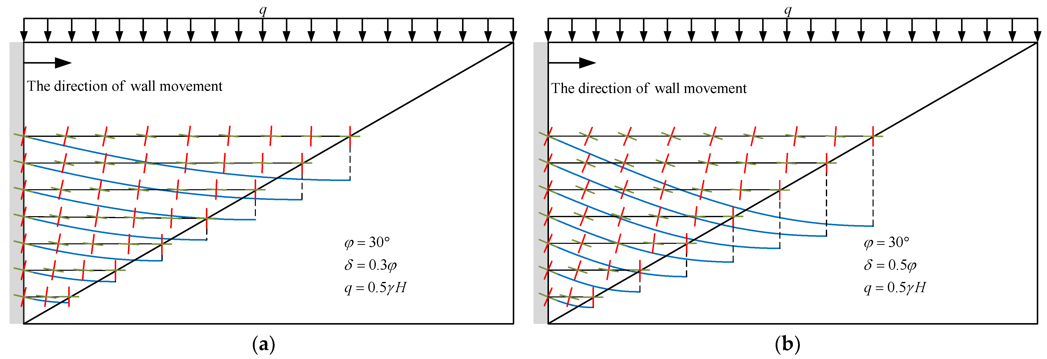
4.1. Soil Internal Friction Angle

Figure 9a–c illustrates the influence of the internal friction angle $\phi$ on the passive earth pressure distribution, the passive earth pressure coefficient $K_p$, and the normalized height of the resultant passive force application point $h_p/H$, respectively.

As the internal friction angle increases from 0 to 40° (Figure 9a), the earth pressure distribution transitions from a linear to a distinctly nonlinear form, with the passive earth pressure gradually increasing. When $\phi =0$, the earth pressure distribution remains linear, and the passive earth pressure coefficient equals 1, a condition that does not exist in practical applications. Additionally, the earth pressure distribution is approximately linear in the upper and middle sections of the wall but becomes nonlinear near the wall heel, where the magnitude of earth pressure increases. The larger the internal friction angle, the more pronounced the curvature of the passive earth pressure distribution. This phenomenon aligns with the enhanced soil arching effect observed with increasing soil–wall friction, where soil arch concentrate load transfer toward the lower wall section.

Figure 9b illustrates the effect of internal friction angle on the passive earth pressure coefficient. As the internal friction angle increases from 0 to 45°, the passive earth pressure coefficient increases monotonically. In addition, a higher surface surcharge q results in a larger $K_p$ value, and the sensitivity from $K_p$ to $\phi$ becomes more pronounced at higher surcharge levels.

As shown in Figure 9c, for a given soil–wall friction angle $\delta$, the normalized height of the application point initially decreases and then increases as the internal friction angle increases. This initial decrease is more evident for smaller values of $\delta$. Notably, the application point starts at H/3 for $\phi =0$, decreases to a minimum, and returns to H/3 at $\phi =90°$. This indicates linear pressure distributions for the theoretical limits of $\phi =0$ (frictionless, similar to hydrostatic) and $\phi =90°$ (infinitely frictional, unrealistic), both of which are rarely observed in practice. As $\delta$ increases, the value of $\phi$ corresponding to the minimum $h_p$ shifts to lower angles.

For typical engineering soils where $\phi$ generally ranges from 20° to 40°, the height of the application point generally decreases with increasing $\phi$.

4.2. Soil–Wall Interface Friction Angle

Figure 10a–c presents the effects of the soil–wall interface friction angle $\delta$ on the passive earth pressure distribution, the passive earth pressure coefficient $K_p$, and the normalized height of the resultant force application point $h_p/H$, respectively, for a constant internal friction angle ($\phi =30°$).

The variation in passive earth pressure distribution with $\delta$ is illustrated in Figure 10a. As $\delta$ increases, the distribution transitions from a linear to a curvilinear profile, with the degree of curvature intensifying at higher $\delta$ values. At $\delta =0$, a linear distribution is observed, consistent with Rankine’s passive earth pressure theory, reflecting no shear mobilization at the wall interface. With increasing $\delta$, the pressure intensity diminishes in the mid-to-upper wall region relative to Rankine’s prediction, while it exceeds Rankine’s values near the wall base. The curvilinear profile suggests a redistribution of stresses, likely driven by enhanced soil arching, which concentrates load transfer toward the lower wall section as wall friction strengthens.

Figure 10b shows a clear non-monotonic relationship between the passive earth pressure coefficient and the soil–wall friction angle. Starting from the Rankine condition at $\delta =0$, $K_p$ increases with $\delta$, reaching a peak value at an intermediate soil–wall friction angle, and then decreases as $\delta$ approaches the internal friction angle $\phi$. This trend reflects the interaction between two competing mechanisms: increasing shear resistance along the wall interface tends to increase passive resistance, while the associated changes in stress state and excessive arching effects may become less efficient for mobilizing overall resistance beyond an optimal $\delta$. The existence of this peak implies that maximizing soil–wall friction does not necessarily yield the highest passive resistance. Additionally, it is observed that, while a higher surface surcharge q consistently increases the magnitude of $K_p$, the location ($\delta$ value) of the peak $K_p$ remains relatively unaffected by changes in surcharge.

The influence of $\delta$ on the normalized height of the resultant force application point is shown in Figure 10c. Similar to the trend observed for $K_p$, this relationship is non-monotonic. Starting from $h_p=H/3$ at $\delta =0$, the application point initially shifts downward as $\delta$ increases from zero. This initial downward shift is consistent with the pressure redistribution observed in Figure 10a, where soil–wall friction causes pressure to concentrate lower on the wall. Beyond a certain value of $\delta$, $h_p$ begins to increase again. With increasing q, the curve retains its shape, but $h_p$ shifts upward, with the increment diminishing at higher loads.

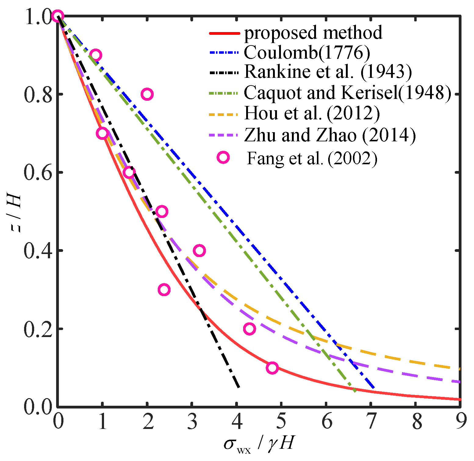
5. Comparison with Existing Theories and Experimental Data

To assess the validity and practical applicability of the passive earth pressure results derived in this study, a comparative analysis was conducted with existing theoretical solutions and available experimental data.

Figure 11 compares the horizontal passive earth pressure distribution obtained from the present study with predictions from Hou et al. [11], Zhu and Zhao [12], and classical approaches, such as the Coulomb, Rankine, and Caquot-Kerisel theories. Classical theories, such as those of Coulomb, Rankine, and Caquot-Kerisel, generally predict linear passive earth pressure distributions against the wall height, although the specific magnitudes vary based on their underlying assumptions regarding wall friction and failure surface geometry. As shown in Figure 11, for the depicted conditions, the results from the Coulomb and Caquot-Kerisel theories are relatively close to each other, and both predict higher pressures than Rankine theory. In contrast, the distributions derived from methods explicitly incorporating soil arching effects, including the present work, Hou et al. [11], and Zhu and Zhao [12], are distinctly nonlinear. These curved profiles predict lower pressures than the classical linear theories in the upper part of the wall. However, they tend to predict significantly higher pressures near the wall base. This deviation from a linear profile reflects a redistribution of stresses attributed to the soil arching mechanism, which decreases pressure in the upper wall region while concentrating it near the base.

Figure 12a presents a comparison of the calculated passive earth pressure coefficient $K_p$ as a function of the internal friction angle $\phi$ against results from the aforementioned theories. All models predict an increase in $K_p$ with increasing $\phi$, reflecting enhanced shear resistance with greater frictional strength. However, significant quantitative differences are observed between the theories. The predictions from Hou et al. [11] yield the highest $K_p$ values, while the results from the Coulomb theory and Zhu and Zhao’s method [12] are closely aligned. The Caquot-Kerisel theory predicts $K_p$ values slightly lower than those of Coulomb. Among all theories compared, Rankine provides the lowest $K_p$ predictions. Notably, the $K_p$ values obtained using the present method lie between the predictions of the Caquot-Kerisel and Rankine theories for the range of $\phi$ considered. The divergence between the predictions from the various theories generally increases at higher internal friction angles.

The influence of $\phi$ on the normalized height of the resultant force application point is compared in Figure 12b. Classical theories yield a constant $h_p=H/3$, independent of $\phi$, consistent with a uniform linear distribution across the wall height. Conversely, $h_p$, from this study and References [11,12], decreases as $\phi$ increases, reflecting a shift in the pressure resultant due to curvilinear distributions. At $\phi =0$, all models converge at $h_p=H/3$, indicative of a cohesionless, frictionless state with no arching. As $\phi$ rises, divergence emerges: the $h_p$ from Hou et al. [11] exhibits the most significant decline, followed by Zhu and Zhao [12] with a moderate reduction, while the present study shows the smallest decrease.

Figure 13a illustrates the effect of the soil–wall friction angle $\delta$ on the passive earth pressure coefficient $K_p$ for a fixed internal friction angle $\phi =30°$. As expected for a smooth wall condition, all theories converge to the same $K_p$ value at $\delta =0$, which corresponds to the Rankine passive earth pressure coefficient. As $\delta$ increases from zero, different trends emerge. The result predicted by Rankine theory shows that $K_p$ remains constant, as wall friction is neglected in the formulation. The Coulomb, Caquot-Kerisel, and Zhu and Zhao theories all predict a similar, gradual monotonic increase in $K_p$ with increasing $\delta$. In contrast, the $K_p$ predicted by Hou et al. [11] increases much more rapidly, showing significant amplification at higher $\delta$ values.

The $K_p$ derived from the present study exhibits non-monotonic behavior, initially increasing with $\delta$ before decreasing as $\delta$ becomes larger. This unique non-monotonic trend is a significant differentiator of the proposed model, contrasting sharply with classical theories and other analyses. It suggests a complex interplay between interface friction and overall stability captured by the current approach.

Figure 13b compares the effect of $\delta$ on the application point height $h_p$. Again, classical theories predict a constant $h_p=H/3$. The other models, including the present work, show $h_p$ generally decreasing as $\delta$ increases from zero. The rate of decrease is most rapid in the results of Reference [11], followed by Reference [12]. The present study predicts the smallest decrease in $h_p$, with the curve tending to flatten at higher $\delta$ values. The application height $h_p$ predicted by the proposed method generally falls between the constant value of H/3 assumed by classical theories and the lower values obtained from other theories that account for nonlinear pressure distributions. This intermediate position for $h_p$ leads to an assessment of overturning resistance that is potentially more balanced than other methods. This offers a potentially advantageous balance between ensuring structural stability and achieving design economy.

Theoretical predictions are compared with experimental data from Fang et al. [27] in Figure 14. The theories of Coulomb and Caquot-Kerisel align reasonably well with the experimental results near the top of the wall, where other theories tend to underestimate the pressure. Predictions by Hou et al. [11] and Zhu and Zhao [12] are similar to each other and provide a better fit for the pressure distribution in the mid-upper portion of the wall. Experimental data points are distributed on either side of the linear prediction from Rankine, which reflects the general trend of increasing pressure with depth. However, this linear approach inherently cannot capture the observed non-linear pressure profile, particularly underestimating values near the wall base. The results from the present study show favorable agreement with the experimental data in the mid-lower sections of the wall, although some deviation is observed around the mid-height.

To quantitatively assess the prediction accuracy of the different theoretical methods against the experimental data from Fang et al. [27], the Sum of Squared Errors (SSE) and the Coefficient of Determination (R²) for the earth pressure distribution, along with the percentage error in the resultant force application height, were calculated (see

Table 1. Comparison of passive earth pressure prediction accuracy among different methods.

	Proposed Method	Coulomb	Rankine	Caquot and Kerisel [1]	Hou et al. [11]	Zhu and Zhao [12]
SSE for earth pressure	3.9272	21.9925	4.2317	14.7391	6.6133	5.149
R2 for earth pressure	0.8108	−0.0595	0.7961	0.2899	0.6814	0.7519
Application height error (%)	−10.12	13.07%	13.07	13.07	−45.33	−24.31

Note: A negative value for application height error indicates that the predicted application height is lower than the experimental result.

). The statistical results indicate that the proposed method yields the lowest SSE and the highest R² value (0.8108), suggesting the best overall agreement with the experimental earth pressure measurements among the compared theories. Notably, the linear Coulomb theory shows a poor fit to the experimental data (R² < 0), while other methods achieve intermediate accuracy. Furthermore, the proposed method also exhibits the smallest percentage error in predicting the application height of the resultant force.

6. Conclusions

This study introduces an analytical method for passive earth pressure using 2D differential element equilibrium, critically eliminating a priori soil arch assumptions. The approach yields the internal stress field and pressure distribution and allows the passive arch shape to be derived analytically from principal stress trajectories. Parametric studies and comparisons with established theories and experimental data validated the method’s effectiveness in capturing essential arching effects and passive earth pressure behavior. The principal conclusions are as follows:

(1)

Owing to the passive arching effect, the limit equilibrium state is achieved only locally near the wall back and lower sliding surface, which contrasts with methods that assume the entire wedge to be in a limit equilibrium state. The derived major principal stress varies in magnitude and direction at constant height.

(2)

The derived passive soil arch shape lies below conventional parabolic/circular assumptions, becoming significantly steeper with increasing soil–wall friction angle. Unlike fixed-geometry assumptions, it is also sensitive to surcharge, reflecting its dependence on the overall stress field.

(3)

The passive earth pressure coefficient increases with the internal friction angle and surcharge, consistent with established theories. However, it shows a non-monotonic relationship with the soil–wall friction angle, peaking at an intermediate value before decreasing.

(4)

Comparisons indicate the proposed method reasonably predicts pressure distributions observed in experiments, notably showing closer agreement in the lower wall regions than other theories.

It should be noted, however, that, due to space constraints, the reasons behind some results remain insufficiently explored, particularly those exhibiting marked deviations from existing theories, such as the non-monotonic trend of $K_p$ with increasing $\delta$. Subsequent work is required to integrate extensive experimental data and numerical simulations to provide a more detailed interpretation and analysis of these theoretical outcomes. Additionally, the assumptions adopted in this study, while facilitating analytical tractability, inevitably introduce certain limitations. The assumptions of plane strain conditions, homogeneous cohesionless soils, planar sliding surfaces, and full mobilization of wall–soil friction simplify the analysis but may not fully reflect complex field conditions such as soil heterogeneity, cohesion effects, irregular failure surfaces, or incomplete interface mobilization. These idealizations restrict the direct applicability, particularly for cohesive or highly heterogeneous backfills, and do not account for 3D effects or complex geometries. Therefore, for practical engineering applications, especially under conditions significantly different from the idealizations, a comprehensive assessment can be achieved by integrating the results of the proposed method with site-specific data or numerical analyses.

References

1. Caquot, A.; Kerisel, J. Tables for the Calculation of Passive Pressure, Active Pressure and Bearing Capacity of Foundations; Gauthier-Villars: Paris, France, 1948. [Google Scholar]
2. Chang, M. Lateral earth pressures behind rotating walls. Can. Geotech. J. 1997, 34, 498–509. [Google Scholar] [CrossRef]
3. Neal, T.S.O.; Hagerty, D.J. Earth pressures in confined cohesionless backfill against tall rigid walls—A case history. Can. Geotech. J. 2011, 48, 1188–1197. [Google Scholar] [CrossRef]
4. Wang, Y. Distribution of earth pressure on a retaining wall. Géotechnique 2000, 50, 83–88. [Google Scholar] [CrossRef]
5. Yang, Y.Z.; Wu, W.B.; Ni, F.F.; Mei, G.X. Pseudo-dynamic analysis of seismic non-limit passive earth pressure under the rb mode. Eng. Mech. 2023. [Google Scholar] [CrossRef]
6. Handy, R.L. The arch in soil arching. J. Geotech. Eng. 1985, 111, 302–318. [Google Scholar] [CrossRef]
7. Liu, H.; Kong, D.; Gan, W.; Wang, B. Seismic active earth pressure of limited backfill with curved slip surface considering intermediate principal stress. Appl. Sci. 2021, 12, 169. [Google Scholar] [CrossRef]
8. Khosravi, M.H.; Kargar, A.R.; Amini, M. Active earth pressures for non-planar to planar slip surfaces considering soil arching. Int. J. Geotech. Eng. 2020, 14, 730–739. [Google Scholar] [CrossRef]
9. Yu, P.; Liu, Y. Analysis of active earth pressure behind rigid retaining walls considering curved slip surface. Geotech. Geol. Eng. 2024, 42, 251–270. [Google Scholar] [CrossRef]
10. Wang, X.; Dang, F.; Cao, X.; Zhang, L.; Gao, J.; Xue, H. Solution for Active and Passive Earth Pressure on Rigid Retaining Walls with Narrow Backfill. Appl. Sci. 2025, 15, 1750. [Google Scholar] [CrossRef]
11. Hou, J.; Xia, T.D.; Kong, X.B.; Sun, M.M. Passive earth pressure on retaining walls calculated by principle of soil arching effect. Rock Soil Mech. 2012, 33, 2996–3000. [Google Scholar] [CrossRef]
12. Zhu, J.M.; Zhao, Q. Unified solution to active earth pressure and passive earth pressure on retaining wall considering soil arching effects. Rock Soil Mech. 2014, 35, 2501–2506. [Google Scholar] [CrossRef]
13. Patel, S.; Deb, K. Experimental and analytical study of passive earth pressure behind a vertical rigid retaining wall rotating about base. Eur. J. Environ. Civ. Eng. 2022, 26, 2371–2399. [Google Scholar] [CrossRef]
14. Han, M.; Chen, X.; Jia, J. Analytical solution for displacement-dependent 3D earth pressure on flexible walls of foundation pits in layered cohesive soil. Acta Geotech. 2024, 19, 5249–5275. [Google Scholar] [CrossRef]
15. Wang, Z.; Kang, W.; Chen, F.; Lin, C. Seismic passive earth pressures of narrow cohesive backfill against gravity walls using the stress characteristics method. Soils Found. 2024, 64, 101505. [Google Scholar] [CrossRef]
16. Tracy, F.T.; Vahedifard, F. Analytical solutions for coupled hydromechanical modeling of lateral earth pressures in unsaturated soils. Comput. Geotech. 2025, 179, 107038. [Google Scholar] [CrossRef]
17. Hu, W.; Hu, T.; Lin, S.; Tang, J.; Zhou, Y.; Hu, Q. Experimental Study on Deformation and Passive Earth Pressure Behind Cantilever Pile Retaining Walls in Narrow Excavations. Geotech. Geol. Eng. 2024, 42, 7041–7061. [Google Scholar] [CrossRef]
18. Dang, F.; Wang, X.; Cao, X.; Gao, J.; Ding, J.; Zhang, L. Calculation method of earth pressure considering wall displacement and axial stress variations. Appl. Sci. 2023, 13, 9352. [Google Scholar] [CrossRef]
19. Xu, J. Investigation into the Displacement-Dependent Lateral Earth Pressure on the Rigid Retaining Wall with Different Modes of Movement: Modeling with the Trigonometric Function. Int. J. Geomech. 2023, 23, 04023166. [Google Scholar] [CrossRef]
20. Li, D.Y.; Ma, Z.H.; Liu, J.; Yin, J.L.; Sun, B.Y. Seismic Rotation Stability of Retaining Wall with Cohesive-frictional Backfill Considering Embedment Depth. Chin. J. Geotech. Eng. 2025. Online. [Google Scholar] [CrossRef]
21. Wu, K.; Yu, P.; Liu, Y. Simulation of Passive Earth Pressure against Retaining Wall Considering Wall Movement Mode. IOP Conf. Ser. Earth Environ. Sci. 2021, 714, 022002. [Google Scholar] [CrossRef]
22. Sahoo, J.P.; Ganesh, R. Discussion of “Estimation of Passive Earth Pressure against Rigid Retaining Wall Considering Arching Effect in Cohesive-Frictional Backfill under Translation Mode” by Yanyan Cai, Qingsheng Chen, Yitao Zhou; Sanjay Nimbalkar, and Jin Yu. Inter. Int. J. Geomech. 2018, 18, 07018011. [Google Scholar] [CrossRef]
23. Dalvi, R.S.; Pise, P.J. Analysis of Arching in Soil-Passive State. Indian Geotech. J. 2012, 42, 106–112. [Google Scholar] [CrossRef]
24. Janssen, H.A. Versuche uber Getreidedruck in Silozellen. Z. Ver. Deut. Ing. 1895, 39, 1045–1049. [Google Scholar]
25. Jaky, J. Pressure in Silos. In Proceeding of the 2nd International Conference on Soil Mechanics and Foundation Engineering, Rotterdam, The Netherlands, 21–30 June 1948; pp. 103–107. [Google Scholar]
26. Pipatpongsa, T.; Heng, S. Granular Arch Shapes in Storage Silo Determined by Quasi-static Analysis under Uniform Vertical Pressure. J. Solid Mech. Mater. Eng. 2010, 4, 1237–1248. [Google Scholar] [CrossRef]
27. Fang, Y.S.; Ho, Y.C.; Chen, T.J. Passive Earth Pressure with Critical State Concept. J. Geotech. Geoenviron. 2002, 128, 651–659. [Google Scholar] [CrossRef]
Figure 1. Schematic comparison of analysis methods: (a) traditional horizontal layer analysis; (b) proposed 2D differential element approach.
Applsci 15 06345 g001
Figure 2. Mohr circle representation of the stress state for a soil element adjacent to the wall (x = 0) under the passive limit equilibrium state.
Applsci 15 06345 g002
Figure 3. Contour plot of the parameter m p .
Applsci 15 06345 g003
Figure 4. Stress distribution within the wedge: (a) vertical normal stress; (b) shear stress; (c) horizontal normal stress; (d) relative stress ratio.
Applsci 15 06345 g004
Figure 5. Stress state of soil element along the soil arch.
Applsci 15 06345 g005
Figure 6. Distribution of principal stress directions and soil arch curves in the sliding wedge: (a) δ = 0.3 φ ; (b) δ = 0.5 φ .
Applsci 15 06345 g006
Figure 7. Schematic diagram of circular arch shape under passive state conditions.
Applsci 15 06345 g007
Figure 8. Comparison of the proposed soil arch shape with the assumed circular and parabolic arches: (a) q = 0.2 γ H ; (b) q = γ H .
Applsci 15 06345 g008
Figure 9. Effect of internal friction angle on passive earth pressure: (a) passive earth pressure distribution; (b) passive earth pressure coefficient; (c) the height of the application point.
Applsci 15 06345 g009
Figure 10. Effect of soil–wall friction angle on passive earth pressure: (a) passive earth pressure distribution; (b) passive earth pressure coefficient; (c) the height of the application point.
Applsci 15 06345 g010
Figure 11. Comparison of passive earth pressure distribution with existing theories [1,11,12].
Applsci 15 06345 g011
Figure 12. Comparison with existing theories [1,11,12] on the effect of internal friction angle on passive earth pressure: (a) passive earth pressure coefficient; (b) the height of application point.
Applsci 15 06345 g012
Figure 13. Comparison with existing theories [1,11,12] on the effect of soil–wall friction angle on passive earth pressure: (a) passive earth pressure coefficient; (b) the height of application point.
Applsci 15 06345 g013
Figure 14. Comparison between theoretical predictions [1,11,12] and experimental results [27].
Applsci 15 06345 g014