Dual Branch Encoding Feature Aggregation for Cloud and Cloud Shadow Detection of Remote Sensing Image

Abstract

Cloud detection is a critical preprocessing step for optical remote sensing imagery. However, traditional CNN-based methods have limitations in global feature modeling, while Transformer models, despite their strong global modeling capability, struggle to capture fine-grained local details effectively. To tackle these challenges, this study introduces a dual-path neural network framework that synergistically combines convolutional neural networks (CNNs) and architectures. By capitalizing on their complementary strengths, this work proposed a dual-branch feature extraction architecture that utilizes two different feature aggregation modes to effectively aggregate features of CNN and Transformer at different levels. Specifically, two novel modules are introduced: the Dual-branch Lightweight Aggregation Module (DLAM), which fuses CNN and Transformer features in the early encoding stage and emphasizes key information through a feature weight allocation mechanism; and the Dual-branch Attention Aggregation Module (DAAM), which further integrates local and global features in the late encoding stage, improving the model’s differentiation performance between cloud and cloud shadow areas. The collaboration between DLAM and DAAM enables the model to efficiently learn multi-scale and spatially hierarchical information, thereby improving detection performance. The experimental findings validate the superior performance of our model over state-of-the-art methods on diverse remote sensing datasets, attaining enhanced accuracy in cloud detection.

1. Introduction

The remarkable progress in scientific and technological domains has propelled revolutionary transformations in remote sensing imaging technologies. Modern remote sensing satellites not only offer higher spatial resolution but also provide high-quality remote sensing imagery across a broader geographical range, delivering unprecedented data support for global environmental monitoring, resource management, and disaster warning applications. This technological progress has significantly expanded the scope of remote sensing research, driving its in-depth development in various application scenarios, such as meteorological disaster monitoring [1], land cover change analysis [2], and natural resource dynamic assessment [3]. Notwithstanding these advancements, the capture and computational analysis of remotely sensed data present persistent challenges that warrant further investigation. Clouds and cloud shadows frequently act as common occlusion factors, often becoming major sources of interference that affect data quality. The presence of clouds may lead to partial or complete loss of ground object information, while cloud shadows can distort ground feature characteristics, resulting in misclassification or information confusion. Such disturbances diminish not only the operational value of remote sensing data products, but also introduce cascading uncertainties that undermine analytical rigor and compromise evidence-based decision-making processes. Specifically, clouds affect the spectral characteristics, morphological structures, and texture information of surface targets to varying degrees, posing significant challenges for high-precision remote sensing data interpretation. Therefore, effectively detecting, segmenting, and restoring cloud and cloud shadow regions has become a critical research topic in remote sensing image processing.

In response to this issue, the scientific community has devised multiple solutions, principally divided into classical cloud and shadow detection algorithms and contemporary deep learning-driven techniques. Conventional cloud detection methodologies are typically classified into three primary categories: statistical methods, spectral threshold-based methods, and morphology, as well as texture-based methods. First, statistical methods primarily include statistical equation methods and clustering analysis methods. The statistical equation method constructs mathematical models using brightness, reflectance, and other feature parameters in remote sensing images, detecting clouds by applying predefined computational formulas [4], and further, cloud shadows are matched to their corresponding clouds based on geometric relationships between them [5,6,7,8,9,10]. Meanwhile, the clustering-based approach segments remote sensing image pixels into discrete categories by jointly analyzing their spectral attributes and spatial arrangement characteristics, thereby identifying and separating cloud regions [11]. These methods are advantageous due to their relatively intuitive mathematical models and suitability for structured data. However, in complex scenarios—particularly when cloud morphology varies significantly or mixed pixels are present—the stability and accuracy of detection may be affected. Spectral threshold-based methods utilize the reflectance differences in clouds across different spectral bands for detection. This analytical framework permits bifurcation into either unimodal temporal scene examination or sequential temporal image assessment paradigms. Single-period image analysis relies on remote sensing data captured at a specific moment, using predefined spectral thresholds in selected bands to distinguish between clouds and surface objects [12,13]. In contrast, multi-temporal image analysis leverages temporal changes in the spectral characteristics of clouds and cloud shadows across different time points for detection [14,15,16]. Spectral threshold methods offer high computational efficiency and are well-suited for large-scale automated processing. However, their effectiveness depends heavily on the spectral characteristics of the images, requiring recalibration of thresholds for different sensor-acquired images. Additionally, their accuracy may be limited when dealing with thin clouds, cirrus clouds, or cloud-shadow confusion. Morphology- and texture-based methods detect clouds and cloud shadows by analyzing their geometric shapes, edge features, and texture information [17]. Clouds typically exhibit soft or diffuse edges, whereas cloud shadows often have a geometric correspondence with cloud positions. Therefore, morphological operators and texture analysis techniques (such as gray-level co-occurrence matrices and Gabor filtering) can be used to differentiate between clouds and background surface features. Furthermore, some researchers have proposed hybrid methods that integrate multiple features—combining spectral, morphological, and texture characteristics—to improve cloud detection accuracy [18]. Despite these advancements, traditional methods still face challenges when dealing with different types of clouds. For instance, thin clouds contain both cloud spectral information and underlying surface details, making them difficult to identify using single-feature detection methods. Moreover, cloud shadows can have spectral similarities with certain surface objects (such as water bodies or shaded areas), leading to misclassification. As a result, traditional methods often require additional discriminative rules to eliminate interference when detecting complex clouds or dynamically changing cloud shadows, which in turn increases computational complexity.

Although traditional statistical, spectral threshold, and morphological texture-based methods perform well on specific datasets, they still suffer from high computational complexity, strong dependency on specific data parameters, and limited generalization ability. Additionally, many of these methods require manually set empirical parameters, which reduces their adaptability across different datasets. With the rapid advancement of big data and artificial intelligence technologies, machine learning and deep learning methods have been increasingly applied to the automatic detection of clouds. Compared to traditional methods, machine learning algorithms can automatically learn data features, eliminating the subjectivity of manually set parameters and significantly enhancing the intelligence of detection processes. Conventional machine learning techniques, encompassing decision trees, random forests, and artificial neural networks, have been extensively employed in cloud classification applications [19,20,21]. However, traditional machine learning methods still primarily rely on spectral features and require manually designed features.

The swift evolution of deep learning has catalyzed the pervasive implementation of artificial neural networks in cloud detection, attributable to their remarkable generalization prowess across heterogeneous scenarios. In contrast to conventional threshold-based approaches, deep learning methods effectively transcend spatiotemporal constraints through data-driven paradigms. The paradigm’s principal strength resides in its capacity for automated hierarchical feature learning directly from input images, facilitating fully integrated end-to-end model optimization [22,23,24]. Notably, the feature extraction mechanism employing Convolutional Neural Networks (CNNs) has demonstrably enhanced the detection accuracy for clouds. For instance, Wang et al. [25] developed a temporal sequence-based methodology for cloud and shadow detection in multispectral imagery, innovatively integrating low-rank sparse decomposition with a Siamese network architecture. By constructing a composite reference image, this approach addresses the challenges posed by dynamic cloud distributions through the integration of DCM and MDFM, enabling robust differential feature extraction while mitigating semantic information attenuation during the decoding process. Jiao et al. [26] innovatively combined the UNet backbone network with a customized Conditional Random Field (CRF) to achieve precise edge segmentation of clouds. Surya et al. [27] introduced a network, CSDUNet, which employs multi-scale feature map concatenation and hierarchical feature extraction to achieve precise pixel-level semantic segmentation of clouds in optical images. Wang et al. [28] proposed MRFA-Net, innovatively designing AFEM and a Multi-scale Attention Mechanism to holistically model both localized patterns and global contextual relationships, effectively addressing multi-scale representation learning challenges in cloud analysis, thereby improving the segmentation accuracy of clouds boundary details. Shi et al. [29] introduced a Selective Kernel (SK) module to capture cloud features of different sizes and designed a Parallel Dilated Convolution Model (PDCM) to enhance the segmentation accuracy of small cloud targets. Additionally, they adopted Content-Aware Reassembly of Features (CARAFE) in the decoder to replace traditional interpolation-based upsampling, effectively restoring fine-grained semantic features. He et al. [30] innovatively integrate the precision of state-space modeling for cloud feature characterization with the computational efficiency of encoder–decoder architectures in feature extraction, providing a new solution for cloud detection. Fan et al. [31] designed Tiny U-shaped Blocks (TUBs) and a Simple Feature Fusion Module (SFFM) to enrich spatial contextual information and optimize semantic features in the encoder. Meanwhile, they employed a lightweight Asymmetric Decoder (ALD) to achieve efficient spatial restoration, significantly achieving concurrent optimization of computational throughput and classification fidelity in cloud detection systems.

In recent years, following the tremendous success of Transformer models in NLP, researchers have begun applying them to computer vision tasks, including semantic segmentation. The Transformer model was initially proposed by Vaswani [32] and his colleagues. Its core mechanism, self-attention, empowers the model to not only process sequential data but also capture global information comprehensively. Moreover, it enables the model to effectively model long-range dependencies, which is a significant advantage in dealing with complex data patterns. Compared to CNN-based semantic segmentation methods, Transformers can more effectively capture global contextual information, addressing CNN’s limitations in handling long-distance dependencies. Against this backdrop, Vision Transformer (ViT) [33] was proposed in 2020; it signified the inaugural application of the Transformer model to computer vision tasks. The central concept of ViT lies in splitting the input image into small patches and transforming these patches into a sequential input that is suitable for the Transformer architecture, enabling global feature modeling. The remarkable success of the Vision Transformer (ViT) has not only established a robust groundwork for the utilization of Transformer models in semantic segmentation tasks but has also ignited the development of a series of innovative segmentation models. This achievement has opened up new possibilities and directions for the field, demonstrating the great potential of Transformer-based architectures in handling complex visual information related to semantic segmentation. Subsequently, models such as TransUNet [34], SegFormer [35], and Swin Transformer [36] were introduced. These methods combine the global modeling capability of Transformers with the local feature extraction advantages of CNNs, significant enhancements have been attained in terms of both the precision of segmentation and the efficiency of computation. Fan et al. [37] proposed a lightweight prior knowledge-guided Transformer model (LPGT), innovatively designing a Prior Knowledge Extraction module (PKE) and a Prior-guided Efficient Attention Block (PEAB). This model, by integrating deep convolution and an extended window-based multi-head self-attention mechanism, reduces the computational burden while enhancing the modeling of long-range dependencies. Li et al. [38] introduced a Transformer-based cloud detection algorithm known as CSDFormer. Innovatively, this algorithm utilizes a hierarchical Transformer structure as its encoder. By harnessing the multi-head self-attention mechanism, the model is able to capture the long-range dependencies between pixels. As a result, it significantly boosts the global contextual comprehension of the semantic relationships between clouds and shadows, enabling a more comprehensive and in-depth understanding of these elements.

With the rapid development of the aforementioned semantic segmentation algorithms, an increasing number of researchers have been applying them to the tasks of cloud segmentation. Gu et al. [39] proposed MAFNet, which extracts features using a combination of ResNet and Transformer. They introduced MAFM and IDAM to enhance small object detection capabilities, while the RGM optimizes boundary segmentation, improving the accuracy of cloud segmentation. The advantages of MAFNet lie in its strengthened feature fusion, enhanced boundary details, and improved small object detection capability. However, it has high computational complexity and still has room for improvement in real-time processing and extreme illumination conditions. Du et al. [40] came up with an innovative convolutional self-attention feature fusion network built upon a U-shaped structure. This method employs a Channel-Spatial Attention Module (CSAM) to adaptively adjust the receptive field and utilizes a Feature Fusion Module (FFM) to combine upsampled and downsampled features, improving edge detail extraction. However, it still faces challenges in the misclassification of highly reflective surfaces such as snow and sand. Liang et al. [41] introduced a cloud detection method based on TSMM, which effectively removes noise and enhances detection accuracy, demonstrating outstanding performance across multiple datasets. However, this method heavily relies on time-series data and may be less effective in scenarios with limited or missing temporal information. Existing studies have demonstrated that CNNs have strong advantages in local feature extraction [42,43,44]. However, due to CNNs’ limitations in global feature recognition, their capability remains constrained. Compared to CNNs, Transformers are not restricted by the local constraints of convolution operations and can better capture the overall contextual relationships within an image, thus improving the model’s ability to grasp global features. Therefore, integrating CNN and Transformer architectures can fully leverage their respective strengths while compensating for their limitations, enhancing model performance in cloud detection tasks.

The main contributions of this paper are as follows:

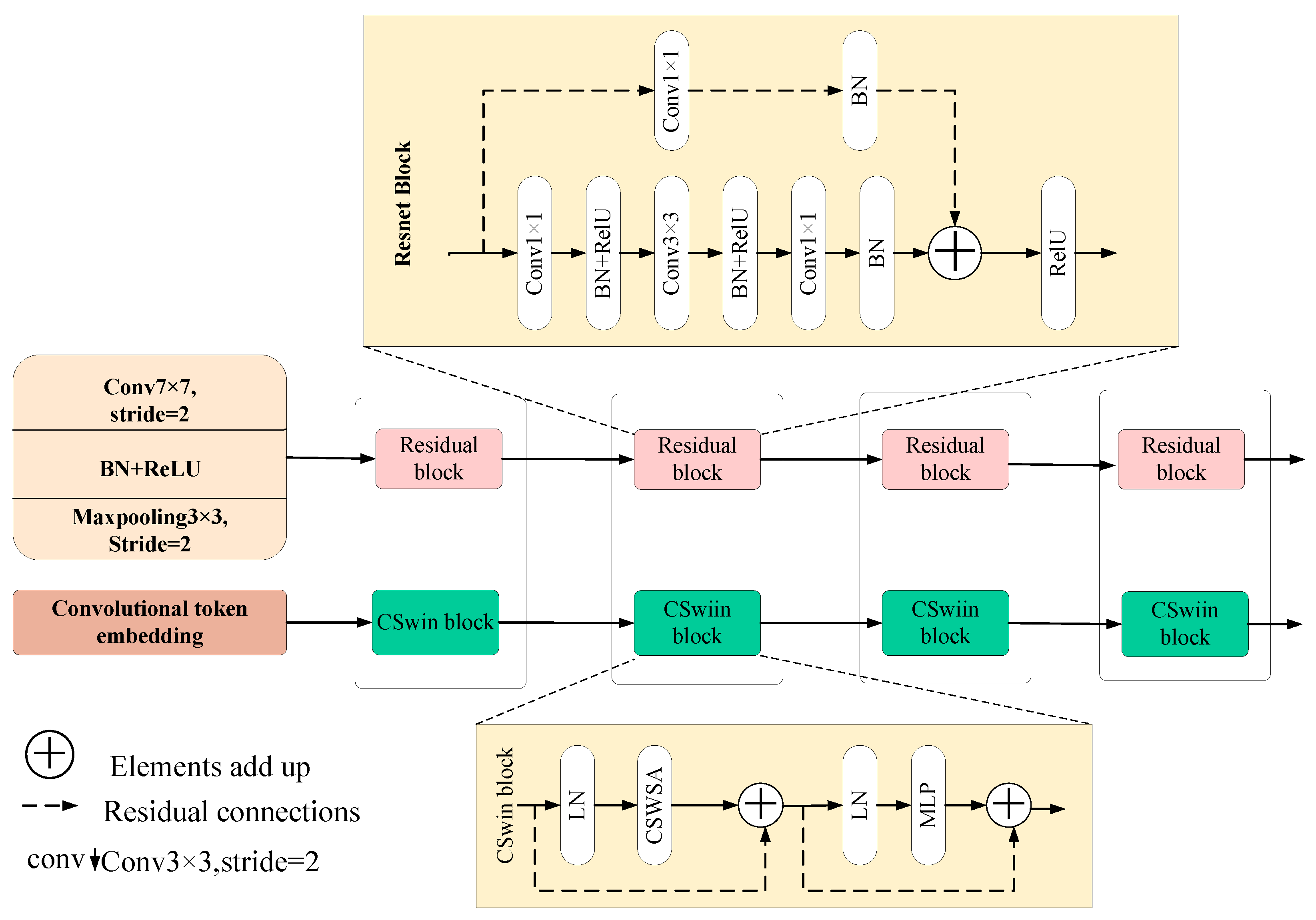
• A novel dual-branch encoding architecture is proposed, combining CNN and Transformer to overcome the limitations of single-backbone models. This architecture incorporates two distinct feature aggregation strategies that effectively fuse multi-level local and global features, thereby enhancing feature representation and segmentation accuracy.
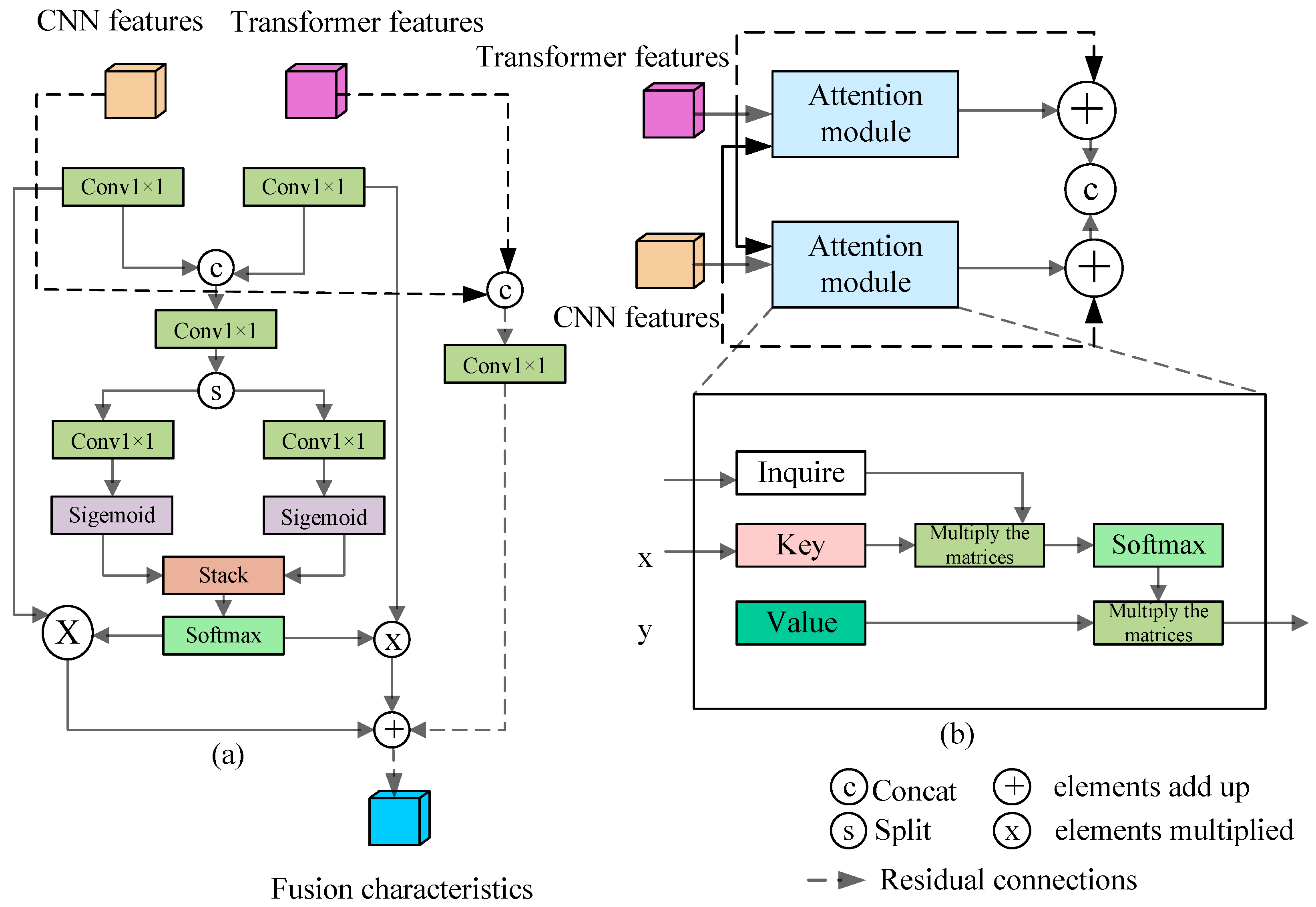
• A Dual-Branch Lightweight Aggregation Module (DLAM) is designed for the early encoding stage. By learning adaptive fusion weights, DLAM emphasizes local features from CNN and global features from Transformer while suppressing irrelevant features, achieving efficient integration with low computational cost.
• A Dual-Branch Attention Aggregation Module (DAAM) is developed for the late encoding stage. Leveraging a self-attention mechanism and weight allocation, DAAM enables interaction and complementarity between the dual-branch features, further improving the fusion of global and local information.

2. Methodology

This study innovatively adopts a dual-branch encoding architecture, constructing separate pathways based on ResNet and CSWin Transformer for local and global feature extraction, respectively. This fully leverages the advantages of both network types and overcomes the limitations of single-backbone models in capturing local details and global context. Unlike previous works that often employ serial or simple fusion strategies, the proposed dual-branch feature aggregation modules—namely the Dual Lightweight Aggregation Module (DLAM) and the Dual Attention Aggregation Module (DAAM)—are designed with differentiated structures for different encoding stages to maintain the relative independence of branch features while enabling efficient and refined fusion. Specifically, the DLAM module adaptively balances local and global information in shallow features through a lightweight weighting mechanism, reducing computational complexity and making it suitable for processing high-resolution inputs. The DAAM module employs a bidirectional self-attention mechanism to facilitate complementarity between deep features, enhancing feature richness and discriminative power. This staged and modular fusion strategy innovatively addresses the performance bottleneck caused by excessive coupling in prior fusion methods, improving sensitivity to complex cloud and cloud shadow patterns. Compared to existing approaches such as Conformer and Mobile-Former, this design demonstrates notable advantages in fusion strategy and network architecture. Moreover, the model incorporates multi-auxiliary supervision branches that effectively mitigate training difficulties in deep networks, ensuring stable and balanced feature learning. This provides strong technical support for cloud detection in remote sensing images. As is vividly depicted in Figure 1, the comprehensive framework of the model, which plays a crucial role in achieving its designed functions, is compartmentalized into an encoding stage, during which initial data processing and feature extraction take place, and a decoding stage, where the processed information is transformed back into a form that can be utilized for the final output. The coding part includes a CNN backbone, a Transformer backbone, and a dual-branch aggregation module. Similar to Transformer framework, CNNs have four stages, each with an output feature map resolution that drops to half that of the previous stage, while increasing the number of channels to twice that of the previous stage. The disparities in features of Convolutional Neural Networks (CNNs) and Transformers across various stages, the model is equipped with two dual-branch aggregation modules, namely the Dual-branch Lightweight Aggregation Module (DLAM) and the Dual-branch Attention Aggregation Module (DAAM). Both aggregation modules are used to more efficiently fuse feature information from two different backbones. The first two coding stages of the project involve the use of dual lightweight modules to fuse the features of Transformer and CNN. Before feature fusion, the module assigns its respective fusion weights to the output features of two different backbones to achieve the purpose of effective aggregation. A dual-branch attention aggregation module is utilized to integrate the feature information from the dual backbones during the final two encoding stages. Prior to the feature integration process, this module makes use of the self-attention mechanism to amalgamate the output features of the CNN and the Transformer. By doing so, it capitalizes on the strong local representation capabilities of the CNN and the powerful global representation capabilities of the Transformer. During the decoding phase, we embark on a step-by-step process to restore the resolution of the feature maps. At the same time, we engage in the seamless integration of the aggregated features from the dual branches across multiple hierarchical levels. To counteract the inevitable loss of boundary and detailed information associated with clouds and cloud shadows, we adopt a downsampling strategy. In a bid to elevate the precision of segmentation, this model ingeniously integrates three supplementary training procedures. These processes are meticulously designed to exercise supervision over the CNN branch, the Transformer branch, and the intermediate decoding stage, ensuring that each component operates optimally and contributes to the overall accuracy of the segmentation task.

2.1. Double-Branched Backbone

The CNN backbone of this model is the Residual Neural Network (ResNet) proposed by He Kaiming and his colleagues. ResNet employs residual connections to link different convolutional layers, aiming to address the issue of degradation in deep convolutional neural networks [45]. We chose ResNet as the CNN branch because of its simple structure and excellent performance. The elaborate architecture of ResNet is presented in Figure 2. In each stage, a certain quantity of residual blocks is included. In the stages ranging from the second to the fourth, within the very first residual block of each stage, the stride of the $3\times 3$ convolutional kernel is deliberately adjusted to 2. This strategic adjustment serves the purpose of diminishing the dimensionality of the feature maps, thereby streamlining the data representation and facilitating more efficient information processing. Once the input image has undergone the initial processes of convolution and pooling, its size is effectively reduced to a mere quarter of its original dimensions. Subsequently, as the data progresses through the second to the fourth stages, a well-orchestrated transformation occurs. The spatial dimensions of the feature maps are systematically halved in comparison to the preceding stage, while concurrently, the number of channels is doubled. This dual change in size and channel count enriches the feature representation, enabling the model to capture more intricate patterns and details within the data. Moreover, through the meticulous adjustment of the number of channels and the quantity of residual blocks within the ResNet architecture, it becomes feasible to craft four distinct ResNet models. These tailored models can be optimized to suit a variety of tasks and datasets, offering enhanced flexibility and performance in different application scenarios. This enables us to select various model sizes based on the requirements of different tasks. Figure 2 illustrates the ResNet architecture, which consists of 3, 4, 6, and 3 residual blocks at each respective stage.

The backbone of the model in this study is CSWin Transformer proposed by USTC [46]. The CSWin Transformer structure is illustrated in Figure 3. The convolutional token embedding processes the input image, which has dimensions of $H\times W\times 3$, resulting in the generation of a feature map with dimensions of $7\times 7$ with a stride of 4. This results in a feature map of size ${\displaystyle \frac{H}{4}}\times {\displaystyle \frac{W}{4}}\times C$ (with C representing the information dimension). The CSwin module includes Layer Normalization (LN), Cross-Shaped Window Self-Attention (CSWSA), and Multi-Layer Perceptron (MLP). LN normalizes the features, enhancing training stability; CSWSA is a lightweight attention mechanism designed to capture both horizontal and vertical dependencies efficiently. It computes the attention relationships between pixels (detailed structure provided below). MLP consists of numerous learnable parameters that capture the learned relationship coefficients. At each interval between stages, the Transformer utilizes a $3\times 3$ convolutional kernel with a stride of 2. This operation downsamples the feature map to half of its original size and, at the same time, doubles the number of channels. Such a strategy allows the features to encompass information across various scales and cuts down on the number of parameters, rendering it well-suited for subsequent semantic segmentation tasks. By adjusting the quantity of CSWin modules in each stage, four distinct scales of CSWin Transformer can be developed: CSWin-T, CSWin-S, CSWin-B, and CSWin-L. The CSWin Transformer has proven its worth in terms of both effectiveness and efficiency, thus becoming the preferred Transformer variant for the models presented in this study.

CSWSA in CSwin is a special self-attention mechanism, as shown in Figure 3. Firstly, the K attention heads $h_i(i\in [1,K])$ in the multi-head self-attention mechanism are divided into two groups, and the cross area is divided into horizontal and vertical bar areas, in which the width of the bar area is controlled by adjusting the SW value. Two sets of attention heads compute local self-attention within horizontal and vertical strip regions, respectively. Local Enhanced Position Encoding (LEPE) is adopted to encode positional information. The function of LEPE is to conduct depthwise separable convolution on the input feature vectors. Subsequently, the features enhanced by LEPE are integrated with the generated attention features via a residual connection. Finally, the outcomes from the horizontal and vertical directions are merged using the Concat operation to generate cross-shaped attention features. In contrast to the full self-attention mechanism, CSWSA cuts down on computational costs, and LEPE enhances the capacity to represent local information.

For the input features $X\in R^{(H\times W)\times C}$, K attention heads are generated by linear projection, and then these attention heads are divided into two groups. One set of attention heads carries out self-attention computation horizontally, and the other set does so vertically. Taking a horizontal self-attention head calculation as an example, the input feature X is split into M (i.e., ${\displaystyle \frac{H}{SW}}$, horizontal bar features $X^i$($i\in [1,M]$), where $SW$ is the width of the horizontal bar region. After that, each horizontal bar feature $X^i$ was self-focused and calculated to obtain the feature $Y^i$. Finally, M features $Y^i$ are spliced together to obtain the output of the k-th horizontal attention head. The formula for calculating the k-th horizontal attention head $H\_Atte{n}_k$ is as follows:

$$\begin{array}{c}X=[X^1,X^2,\dots ,X^M],\mathrm{where}X\in R^{(H\times W)\times C},X\in R^{(SW\times W)\times C},M={\displaystyle \frac{H}{SW}}\hfill \end{array}$$

(1)

$$Y_k^i=Atten(X^i{W}_k^Q,X^i{W}_k^K,X^i{W}_k^V),i\in [1,M]$$

(2)

$$Atten(Q,K,V)=softmax\left({\displaystyle \frac{Q{K}^T}{\sqrt{d}}}\right)\times V+DWconv\left(V\right)$$

(3)

$$H\_Atte{n}_k\left(X\right)=[Y_K^1,Y_K^2,\dots ,Y_K^M]$$

(4)

where $X^i{W}_k^Q,X^i{W}_k^K$, and $X^i{W}_k^V$ represent the projection matrix of queries, keys, and values for the k-th attention head, and DWConv for the depth separable convolution. The formula for calculating the vertical attention head is similar to the one above, with the only difference being the width of the initial split input feature, i.e., M becomes ${\displaystyle \frac{W}{SW}}$·${\displaystyle \frac{K}{2}}$ horizontal attention head and ${\displaystyle \frac{K}{2}}$ vertical attention head are concatenated to form the output of CSWSA, and the formula is as follows:

$$CSWSA\left(X\right)=Concat(h_1,\dots ,h_k)W^0,W^0\in R^{C\times C}$$

(5)

$$h_k=\left\{\begin{array}{ccc}\hfill H\_Atte{n}_k\left(X\right)& & k\in [1,{\displaystyle \frac{K}{2}}]\hfill \\ \hfill V\_Atte{n}_k\left(X\right)& & k\in [{\displaystyle \frac{K}{2}}+1,K]\hfill \end{array}\right.$$

(6)

where $W^0$ represents the projection matrix, $h_k$ represents the k-th attention head, and $H\_Atte{n}_k$ or $V\_Atte{n}_k$ represents the k-th horizontal or vertical attention head calculation. This kind of cross-cutting window effectively expands the attention range of word vectors, and also greatly reduces the computational cost of the attention mechanism.

2.2. Two-Branch Feature Aggregation Module

The two-branch feature aggregation module is divided into the two-branch lightweight aggregation module (DLAM) and the dual-branch attention aggregation module (DAAM), which are utilized to blend the features originating from the CNN and Transformer. DLAM is used for the first and second stages of bipolar fusion, and its lightweight design allows it to be applied to shallow features without burden. DLAM is designed to learn the weights of features from the CNN and Transformer. It places more emphasis on the local features of CNN and the global features of Transformer, while de-emphasizing the less significant features. DAAM, a feature reconstruction module leveraging the self-attention mechanism, is used to merge the dual-branch features from the third and fourth stages. By leveraging self-attention, DAAM captures the beneficial feature information from both CNN and Transformer, allowing CNN to gain global insights from Transformer and enabling Transformer to receive local insights from CNN.

The detailed structure of DLAM is presented in Figure 4a. Initially, the output features from Stages 1 and 2 of the CNN and Transformer undergo a $1\times 1$ convolution operation. This operation serves to modify the channel count of the features. Subsequently, the two sets of features are concatenated and then passed through another $1\times 1$ convolution. This process is beneficial for the interaction between the features from the CNN and the Transformer. Subsequently, the combined features are segmented along the channel dimension through the Split operation. Then, the two separated features are processed, respectively, by a $1\times 1$ convolution and a Sigmoid function, normalizing them so that their pixel values are within the range of 0~1. This is done to prevent the appearance of extreme maximum or minimum values. Next, the two separated features are connected in parallel along the channel dimension by means of the stack operation. Subsequently, the Softmax function is employed to create a pixel-level mixed-weight map, so that the fusion weight maps of the CNN and the Transformer sum up to 1 at the corresponding pixel positions. In the end, the two generated feature fusion weight maps are multiplied pixel by pixel with the first two input features, reallocating the weights to the features of the CNN and the Transformer, thus enabling a more optimal dual-branch fusion. In addition, we employ residual connections (represented by dashed lines) to incorporate earlier features, which helps speed up model optimization and makes it easier to learn the weights of feature graphs.

DAAM is composed of two fundamental attention modules along with two branches for global and local interactions, as illustrated in Figure 4b. The attention module receives inputs from the CNN and Transformer features. Initially, the input X undergoes a $1\times 1$ convolution to create a query matrix, while Y is processed through two $1\times 1$ convolutions to produce a key matrix and a value matrix, respectively. Next, the query matrix is transposed and multiplied by the key matrix to form an attention map, which is then normalized using the Softmax function. Overall, this process allows the input feature y to be reweighted by incorporating information from feature x. Therefore, when x comes from the third or fourth stage Transformer, and y comes from the third or fourth stage CNN, This process is designed to integrate the global information inherent in the Transformer to fine-tune the local features of the Convolutional Neural Network (CNN), facilitating a seamless transition from the global perspective to the local one. Conversely, when the feature representation x is sourced from the CNN and the feature representation y is derived from the Transformer, both within the third or fourth stage, the objective of this process is to leverage the local information of the CNN to refine the global features of the Transformer, thereby achieving a progression from the local to the global context. Ultimately, through these two complementary processes—transitioning from global to local and from local to global—features from the CNN enriched with global information and features from the Transformer augmented with local information are successfully generated. These two sets of features are then combined using residual concatenation, and the Concat operation is applied to merge them, resulting in the final output after a $1\times 1$ convolution.

To assess the performance of the two-branch aggregation module, we visualized the cloud heat map of the model in this study and compared it with the cloud heat map of the features produced by the CNN and Transformer, illustrated in Figure 5. In a heat map, the heavier weights appear redder, while the lighter weights are more blue. From Figure 5, we can see that CNNs usually focus on cloud shadow edges and details, although Transformers typically concentrate on larger targets; this brings to light the distinct merits of Convolutional Neural Networks (CNNs) and the Transformer architecture when it comes to processing local and global data. The model in this study fuses these two features through the two-branch aggregation module, so it combines the advantages of these two networks, and its final segmentation effect is improved compared with the first two.

2.3. Decode Module

During the decoding phase, if the final output feature map is directly upsampled as the prediction result, the segmentation region will be coarse, because although the deep feature has rich semantic information, it has low resolution and thus loses a certain amount of spatial information. The feature map in the early stage of encoding contains rich position information, so we can improve the final prediction effect by fusing the feature map of different coding stages. The internal structure of the decoder in this study is shown in the left area of Figure 6, which will pass through the $3\times 3$ convolutional kernel, BN layer, and ReLU activation function from the deep and shallow input feature maps of the coding stage, respectively. The input feature map from the deep layer is then upsampled, and the dimensions are restored to match the dimensions of the shallow feature map. Finally, the two Concat input feature maps were spliced together and then passed through the $1\times 1$ convolution kernel, BN layer, and ReLU activation function to adjust the channel size. Through the decoder, the model in this study fuses the features of the four coding stages layer by layer to form the final output feature map, and then adjusts the number of channels to the number of categories through the segmentation head to obtain the prediction effect map. The segmentation head in the decoding stage consists of a $1\times 1$ convolutional kernel and an upsampling function (increasing the size to match that of the input image), as shown in the right area of Figure 6. The segmentation head is used to convert the feature map into a predictive image.

3. Experiments

3.1. Datasets

In this experiment, three datasets were used to evaluate the performance of the network algorithm. All three datasets provide labeled data down to the pixel level, and one is a high-resolution Cloud and Cloud Shadow dataset from Google Earth for comparative experiments. The other two sets are publicly available remote sensing image datasets, HRC_WHU and SPARCS, which are used for generalization experiments.

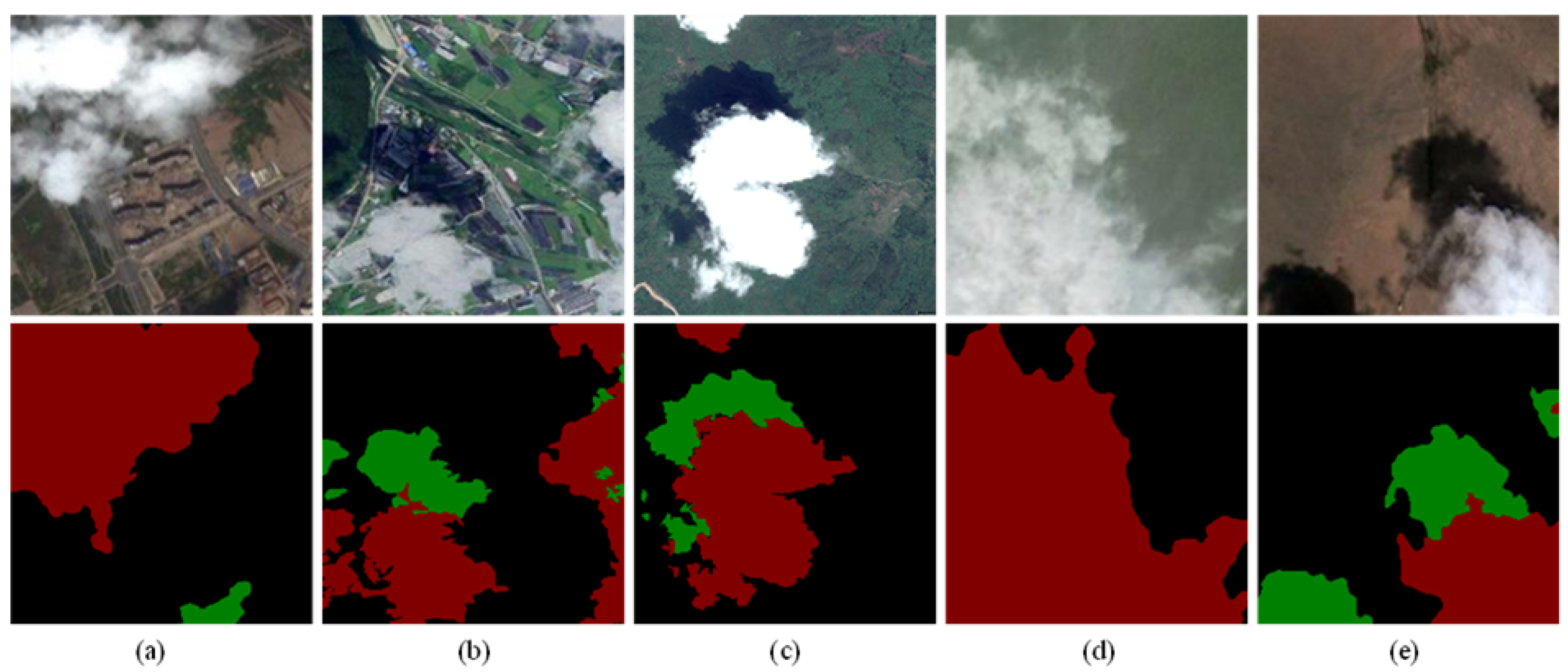
Cloud and Cloud Shadow datasets: The Cloud and Cloud Shadow datasets, which were collected by our research team, focus on plain areas within China and are used to evaluate the core segmentation performance of our method. The majority of the imagery within these datasets is sourced from the QuickBird and WorldView-4 satellites. As presented in

Table 1. Specific parameters of satellite imagery for Cloud and Cloud Shadow datasets.

Satellite Type	Band Number	Band Name	Wavelength Range (nm)	Spatial Resolution (m)
QuickBird	1	blue	450–520	0.61
	2	green	520–600
	3	red	630–690
	4	Near-infrared waves	760–900
WorldView-4	1	blue	50–510	0.3
	2	green	510–580
	3	red	655–690
	4	Near-infrared waves	780–920

, it details the band information for the QuickBird and WorldView-4 satellite images. To guarantee the credibility of the experimental outcomes, we randomly picked 50 high-resolution remote-sensing images as the initial data. These images are situated in the plain regions of China, and their resolutions span from 0.3 m to 30 m. The selected imagery covers five remotely sensed backgrounds, including cities, farmland, vegetation, water, and wasteland.

We manually labeled each of the 50 selected images and categorized them into three categories: background, cloud, and cloud shadow. This annotation was carried out by five annotators working in the field of remote sensing imagery. Each annotator tags the image independently. In the event of a disagreement, the commentators discuss it until an agreement is reached. The decision-making process relies on full consistency, which means that the tag needs to be agreed upon by all annotators before it can be added to the label diagram. Figure 7 selects five sets of original images and their labels in different remote sensing backgrounds in the Cloud and Cloud Shadow datasets. Considering that the experiment would be limited by memory, we cropped the original image to a size of $224\times 224$ pixels and took the RGB three channels. Ultimately, a total of 1916 images underwent cropping and filtering procedures. Out of these, 1545 images were designated for the training phase, while 371 images were earmarked for the testing phase.

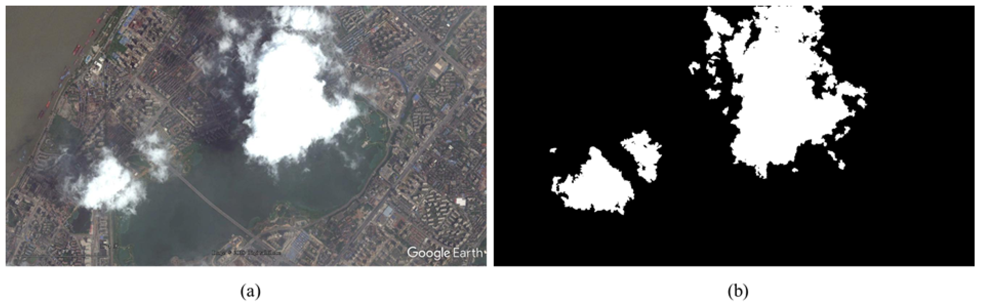
HRC_WHU: Each image is $1280\times 720$ pixels in size and consists of RGB three channels with a resolution between $0.5$ m and 15 m collected from various locations around the world. The researchers divided the image background into five main land types, namely snow, urban, wasteland, vegetation, and water. Figure 8 shows a set of original images and labels. The cloud areas of the label map are marked in white. Due to memory limitations, we cropped 150 high-resolution images from the HRC_WHU dataset to 3488 images with a size of $224\times 224$ pixels. The number of training and validation sets is divided into $4/1$ ratios, with 2791 and 697 images, respectively.

SPARCS: The SPARCS dataset was developed and made available by a research group at Oregon State University. It consists of globally distributed Landsat 8 imagery from the years 2013 to 2014. The dataset contains 80 images, each with a size of $1000\times 1000$ pixels, covering a total of 64 scenes. The images were randomly selected from Landsat 8 satellite imagery between 2013 and 2014.

Table 2. Specific parameters of satellite imagery from the SPARCS dataset.

Band Number	Band Name	Range (nm)	Spatial Resolution (m)
B1	Coastal waves	0.433–0.453	30
B2	Rambo	0.450–0.515	30
B3	Green Wave	0.525–0.600	30
B4	Red Wave	0.630–0.680	30
B5	Near-infrared waves	0.845–0.855	30
B6	SWIR 1	1.560–1.660	30
B7	SWIR 2	2.100–2.300	30
B8	Panchromatic waves	0.500–0.680	15
B9	Cirrus waves	1.360–1.390	30
B10	Thermal Infrared 1	10.60–11.19	100
B11	Thermal Infrared 2	11.50–12.51	100
B12	New Band 1	1.610–1.670	20
B13	New Band 2	2.100–2.200	20
B14	New Band 3	3.900–4.000	60
B15	New Band 4	4.500–4.800	60
B16	New Band 5	8.000–8.500	120

shows the details of each band in the SPARCS dataset.

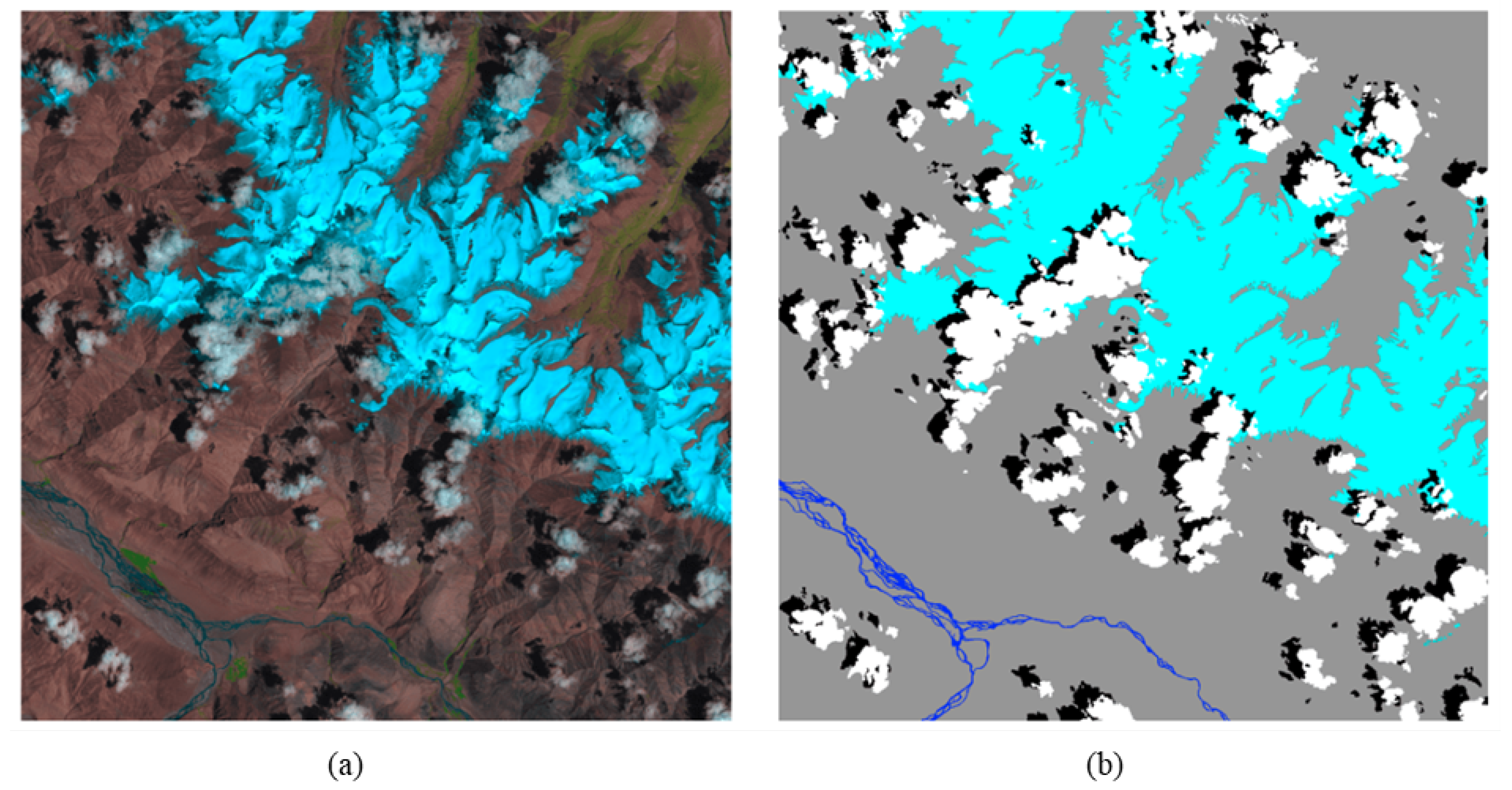
The preview images in the SPARCS dataset are pseudo-color imagery, which maps shortwave infrared waves 1 (B6), near-infrared waves (B5), and red waves (B4) to RGB channels, thereby enabling the visualization of different feature types and providing key information for subsequent accurate classification. In the process of labeling, the tagger relies entirely on visual interpretation, avoiding the problem of incorrect labeling that can be caused by automatic threshold handling. The pixels in the image are labeled with seven categories, which are clouds, cloud shadows, cloud shadows on water, snow/ice, floods, and backgrounds. Since the two categories of flood and water cloud shadow account for only $1.8\%$ and $0.24\%$, we merged them into water and cloud shadow, respectively. The merged label chart contains five categories, and

Table 3. The table that corresponds to the labels and categories of the SPARCS dataset.

Pixel Value	Category	Color	Percentage
0	Cloud	white	21%
1	Cloud Shadow	black	7%
2	Snow/ice	cyan	6%
3	Water	blue	4%
4	Background	grey	62%

shows the corresponding tables of labels and categories. Due to memory limitations, we cropped 80 images from the SPARCS dataset into sub-images of $256\times 256$ pixel size, resulting in a total of 1280 images. Due to the limited training data, the experimental model is prone to overfitting, so we expanded the SPARCS dataset. We used techniques such as random rotation and vertical and horizontal flipping to expand the original 1280 images to 3168 images. Among them, the training set and the validation set have 2534 and 634 images, respectively. Figure 9 shows a set of original preview and label plots in the SPARCS dataset.

3.2. Implementation Details

All of the research in this paper was conducted on computer devices equipped with NVIDIA GeForce RTX 3080, operating system Windows 10, and software platform PyTorch 1.10.0. In this work, the model is trained separately for each dataset. Each dataset requires a model trained from scratch, as the datasets differ in characteristics, and a single model cannot be applied across all of them. In this study, the Adam optimizer was selected as the optimization algorithm for model training. We use the exponential decay algorithm. The exponential decay algorithm is calculated as follows:

$$lr=l{r}_{init}\times {(1-{\displaystyle \frac{epoch}{max\_epoch}})}^{power}$$

(7)

Here, $lr$ and $lr\_init$ represent the current and initial learning rates, respectively; $epoch$ denotes the current number of iterations; $max\_epoch$ indicates the total number of iterations; $power$ is used to control the shape of the curve and is set to 2.

In this experiment, the initial learning rate is set to 0.0001, the total number of iterations is set to 200, the number of samples for a training session is set to 16, and the parameter sum of the Adam optimizer is set to $0.9$ and $0.999$, respectively. Cross-entropy was chosen as the loss function in training. The expression of the cross-entropy loss function is

$$L=-{\displaystyle \frac{1}{N}}\sum _{i=1}^N\sum _{c=1}^M{y}_{ic}log\left(P_{ic}\right)$$

(8)

where N is the total number of training samples.

The final loss function formula is as follows:

$$L_f\left(\theta \right)=L_m\left(\theta \right)+\sum _{i=1}^4{L}_{a_i}\left(\theta \right)+{\displaystyle \frac{\lambda }{2}}{\parallel \theta \parallel }^2$$

(9)

where $L_f$ denotes the final loss function; $L_m$ represents the main loss from the primary branch; $L_{a_i}$ denotes the loss from the i-th auxiliary branch; and $\theta$ refers to the network parameters. The coefficient $\lambda$ in the L2 regularization term is set to 1 by default, and its effectiveness has been validated through a sensitivity analysis presented in the Section 3.3.

To improve feature learning at multiple stages, four auxiliary loss branches are added to the outputs of intermediate layers from the ResNet encoder. Each auxiliary branch computes a cross-entropy loss. The final loss is the sum of the main loss and all auxiliary losses, along with an L2 regularization term. All loss terms are equally weighted by default, without additional balancing coefficients. This design encourages consistent optimization across the network and stabilizes training.

Some commonly used semantic segmentation evaluation indicators are used to evaluate and compare the prediction results of network models in image segmentation tasks. Pixel Accuracy (PA) is the percentage of all correctly categorized pixels out of the total number of pixels. Precision (P) is the percentage of accurately predicted pixels in each class out of the total number of predicted pixels in that category. Recall (R) is the percentage of accurately predicted pixels in each class out of the total number of pixels in that class. Mean Precision (mP) is the average of the precision (P) of all classes. Mean Recall (mR) is the average of the recall (R) for all classes. These metrics are calculated as follows:

$$\mathrm{PA}=\sum _{i=1}^k{\displaystyle \frac{p_{ii}}{{\sum }_{j=1}^k{p}_{ij}}}$$

(10)

$${\mathrm{P}}_{\mathrm{i}}={\displaystyle \frac{p_{ii}}{{\sum }_{j=1}^k{p}_{ij}}},i=1,\dots ,k$$

(11)

$${\mathrm{R}}_{\mathrm{i}}={\displaystyle \frac{p_{ii}}{{\sum }_{j=1}^k{p}_{ij}}},i=1,\dots ,k$$

(12)

$$\mathrm{mP}={\displaystyle \frac{1}{k}}\sum _{i=1}^k{P}_i$$

(13)

$$\mathrm{mR}={\displaystyle \frac{1}{k}}\sum _{i=1}^k{R}_i$$

(14)

The F1 score is the harmonic mean of P and R. It is calculated as follows:

$$\mathrm{F}1={\displaystyle \frac{1}{k}}\sum _{i=1}^k{\displaystyle \frac{2\times P_i\times R_i}{P_i+R_i}}$$

(15)

IoU is the ratio of the intersection and the union of the predicted value and the true value of each category. MIoU is the average of IoU for all classes. FWIoU is a weighted average of IoU based on the frequency of each category in the overall dataset, which allows for a more balanced consideration of the importance of different categories. They are calculated as follows:

$$\mathrm{IoU}={\displaystyle \frac{P_{ii}}{{\sum }_{k=1}^k{P}_{ij}+{\sum }_{j=1}^k{P}_{j}i-Pii}}$$

(16)

$$\mathrm{MIoU}={\displaystyle \frac{1}{k}}\sum _{i=1}^{k}Io{U}_i$$

(17)

$$\mathrm{FWIoU}={\displaystyle \frac{1}{{\sum }_{i=1}^k{\sum }_{j=1}^k{P}_{ij}}}\sum _{i=1}^k\left(IoU\sum _{i=1}^k{P}_{ij}\right)$$

(18)

3.3. Ablation Study

Due to the large differences in the output features of CNN and Transformer, directly merging these two features will lead to poor model performance. Existing methods, such as Conformer [47] and Mobile-Former [48], essentially interact with CNN and Transformer branches from the shallow to the deep layers of the network. This method destroys the independence of CNN and Transformer, and makes their respective advantages gradually disappear. Therefore, we designed the Dual Lightweight Aggregation Module (DLAM) and the Dual Attention Aggregation Module (DAAM) to fuse the features of CNN and Transformer without affecting their respective training. In the ablation experiment, we verified the model performance of DLAM and DAAM at different locations, and also explored the different internal structure settings of DLAM and DAAM. The first two rows of

Table 4. Ablation results of DLAM and DAAM at different positions.

Model	DLAM	DAAM	MIoU (%)
ResNet-50	/	/	92.18
CSWin-T	/	/	92.55
ResNet-50 + CSWin-T	/	/	92.34
	1,2,3,4	/	93.50
	1,2,3	4	93.76
	1,2,4	3	93.68
	1,2	3,4	94.13
	1,3	2,4	93.75

show the segmentation accuracy of the ResNet-50 and CSWin-T benchmark models on Cloud and Cloud Shadow datasets, respectively. From the data in the third row, it can be seen that the evaluation index MIoU of the model without the two-branch feature aggregation module is lower than that of the model using only CSWin-T. This shows that simply fusing the Transformer branch and the CNN branch does not improve the detection effect, but reduces the performance of the model. The next five rows of data permutate and combine DLAM and DAAM in four fusion stages to explore their impact on model performance at different locations. In the DLAM and DAAM columns, we use “/” to indicate the module without markers, and use numbers 1~4 to indicate that the modules using markers fuse the output features from the CNN and the Transformer in the fusion stage of the corresponding numbers. As can be seen from the data in the fourth row, the MIoU increased by $1.16\%$ after using DLAM instead of the coarse fusion method at each stage. This proves the effectiveness of DLAM. Rows 5 and 6 replace the feature aggregation modules of stages 4 and 3 with DAAM, further improving the performance of the model. When DAAM was used in both stages 3 and 4, the optimal MIoU of $94.13\%$ was obtained. These data all confirm that the use of DAAM for two-branch fusion is more effective than the use of DRAM alone.

• It is important to note that the effect of DAAM is related to its position in the fusion phase. The fifth and last rows of Table 4 show that the models using DAAM in the second and fourth fusion phases are not as good as the models using DAAM in the fourth fusion phase. This is because DAAM is essentially an attention module and is generally more effective for features with rich semantic information (such as output features from CNNs and Transformer stages 3 and 4), while increasing DAAM too much will lead to increased complexity of the model and is prone to overfitting. At the same time, when DAAM is used in shallow networks (stages 1 and 2 of the model in this study), the computational burden of the module increases dramatically due to the high resolution of the output feature map of CNN and Transformer. Therefore, as a lightweight fusion module, DLAM is suitable for fusing shallow feature information in stages 1 and 2. Although DAAM has better performance, it is computationally intensive and suitable for integrating rich semantic features in stages 3 and 4.

In order to explore the optimal module structure of DLAM and DAAM, we verified the influence of their different internal structures on the model performance, and the experimental results are shown in

Table 5. Ablation results of DLAM and DAAM with different internal structure settings.

DLAM	DAAM			MIoU (%)
Residual Connections	Upper Branch	Lower Branches	Fusion Methods
✓		✓	Concat	93.44
✓	✓		Concat	93.61
✓	✓	✓	Concat	94.13
✓	✓	✓	Add	93.28
	✓	✓	Concat	93.58

. The third and fifth rows show that the DRAM with the residual structure has a $0.55\%$ higher MIoU than the DLAM without the residual structure. The experimental data proves the effectiveness of the residual structure on DLAM, which is mainly due to the fact that the residual connection can accelerate the convergence of the network and improve the training effect of the model. Above this study, Figure 4b shows the internal structure of a DAAM. Specifically, DAAM has two branches: the upper branch integrates local features from CNN into the output feature map of the Transformer, and the lower branch integrates the global features from the Transformer into the output feature map of the CNN. The data in the first three rows of Table 5 show that the MIoU of DAAM models with only lower and upper branches are $93.44\%$ and $93.61\%$, respectively, which are lower than those of DAAM models with both upper and lower branches. This suggests that CNN and Transformer can improve the performance of the model by complementing each other’s feature expressions.

Once the fused features of the upper and lower branches are acquired, there exist two distinct approaches, namely “Concat” and “Add”, for further integrating these features. The data in the third and fourth rows vividly illustrate the performance of the models utilizing these two fusion methods. Notably, the Mean Intersection over Union (MIoU) value of the model adopting the “Add” method is 0.3 units lower than that of the model implementing the “Concat” method. This clear disparity strongly indicates that within the DAAM architecture, the “Concat” fusion approach demonstrates a superior performance compared to the “Add” fusion approach. The underlying cause of this performance divergence can be attributed to the fundamental differences in how these two operations handle feature integration. Specifically, the “Concat” operation combines the fused features of the CNN and Transformer along the channel dimension. This strategic concatenation effectively safeguards and retains the original characteristic information of both components, allowing for a more coherent and intact representation of the features. On the contrary, the “Add” operation merges the two sets of features through element-wise addition. This process, while seemingly straightforward, has the potential to muddle and obscure the distinctiveness between local and global feature information, thereby resulting in a less optimal performance in terms of segmentation accuracy, as reflected by the MIoU metric. Based on the above, we finally determined the optimal structure settings of DLAM and DAAM through the ablation experiments of different internal structures.

To assess the influence of the L2 regularization strength $\lambda$ on model performance and convergence, we conducted a sensitivity analysis on the Cloud and Cloud Shadow datasets. We tested five values of $\lambda$: $\{0,0.01,0.1,1,10\}$ and recorded final F1 scores, Mean Intersection over Union (MIoU), and convergence epochs.

As shown in

Table 6. Performance under different values of $\lambda$ on the Cloud and Cloud Shadow datasets.

Lambda ($\mathit{\lambda }$)	F1 Score (%)	MIoU (%)	Convergence Epoch
0	96.25	92.90	30
0.01	96.70	93.60	27
0.1	96.90	93.95	25
1	96.97	94.13	23
10	96.40	93.30	32

, a moderate value of $\lambda$ (e.g., 0.1 or 1) leads to better convergence speed and improved segmentation performance. In contrast, too small a $\lambda$ results in insufficient regularization, while too large a value suppresses learning capacity and slows convergence. This experiment validates the robustness of our loss formulation and justifies the default choice of $\lambda =1$ in our method.

To further verify the effectiveness of the auxiliary losses, we conducted an ablation experiment by removing all four auxiliary supervision branches and keeping only the main loss. As shown in

Table 7. Effect of auxiliary losses on model performance on Cloud and Cloud Shadow dataset.

Setting	F1 Score (%)	MIoU (%)
With auxiliary losses (ours)	96.97	94.13
Without auxiliary losses	96.12	93.20

, removing the auxiliary losses leads to a noticeable drop in both MIoU and F1 score, confirming their positive contribution to model performance.

The ablation experiments systematically validate the contributions of the proposed dual-branch aggregation modules, DLAM and DAAM, to the overall model performance. Compared with directly merging features from both branches, the DLAM module, through its lightweight weighting mechanism, effectively enhances the quality of shallow feature fusion. This verifies its innovative advantage in maintaining feature independence while balancing local and global information. The DAAM module serves as the core fusion unit for deep features, leveraging a bidirectional self-attention mechanism to enable in-depth interaction between CNN and Transformer features, significantly improving the model’s capability in delineating cloud and cloud shadow boundaries.

This study is the first to propose and systematically evaluate a two-module staged fusion strategy, combining residual connections and concatenation operations, which substantially optimizes the expressive power of fused features and stabilizes network training. The ablation results demonstrate that this novel design significantly improves key metrics such as MIoU, confirming its practical value and theoretical significance in cloud detection. Compared with existing related fusion strategies, our method achieves performance gains while maintaining computational efficiency, showing excellent engineering applicability.

In addition, a sensitivity analysis on the L2 regularization parameter was conducted to further understand its impact on model convergence and segmentation performance. Results indicate that moderate L2 regularization values (e.g., $\lambda$ = 0.1 or 1) strike a balance between preventing overfitting and maintaining sufficient learning capacity, leading to faster convergence and better segmentation metrics. Too small a regularization value results in under-regularization and slower convergence, whereas excessively large values suppress learning and degrade accuracy. This analysis validates the robustness of our loss formulation and supports the default choice of $\lambda$ = 1 in the training process, contributing to the overall effectiveness and stability of the model.

3.4. Comparative Experiments

In the comparative experiment, we evaluated and contrasted the performance of several prevalent segmentation networks that utilize the Transformer backbone on the Cloud and Cloud Shadow dataset. The outcomes of the experiment are illustrated in

Table 8. Experimental results are compared with the segmentation network based on CNN and CNN+Transformer on Cloud and Cloud Shadow datasets.

Model	PA (%)	mP (%)	mR (%)	F1 (%)	MIoU (%)	FWIoU (%)
Segmenter	96.68	93.56	92.87	93.20	87.39	89.97
PVT	95.54	94.12	94.88	94.49	89.63	91.53
CvT	96.27	95.25	95.65	95.44	91.33	92.84
Swin	96.65	95.98	95.87	95.93	92.20	93.55
CSWin	96.81	96.06	96.17	96.11	92.55	93.84
Our	97.51	96.98	96.86	96.97	94.13	95.15

. Among these networks, the Schizont is a semantic segmentation network characterized by its pure Transformer architecture, and the backbone of it is Vision Transformer (ViT), which still uses the Transformer form in the decoding stage [49]. Compared with ViT, PVT (Pyramid Vision Transformer) adopts a pyramid architecture similar to that of CNN, which enables it to reduce computational complexity in image segmentation and detection tasks [50]. The Convolutional vision Transformer (CvT) adds some convolution operations on the basis of ViT, that is, convolutional token embedding before each stage and convolutional projection is added inside each self-attention module, so that the Transformer can take into account the advantages of CNN [51]. 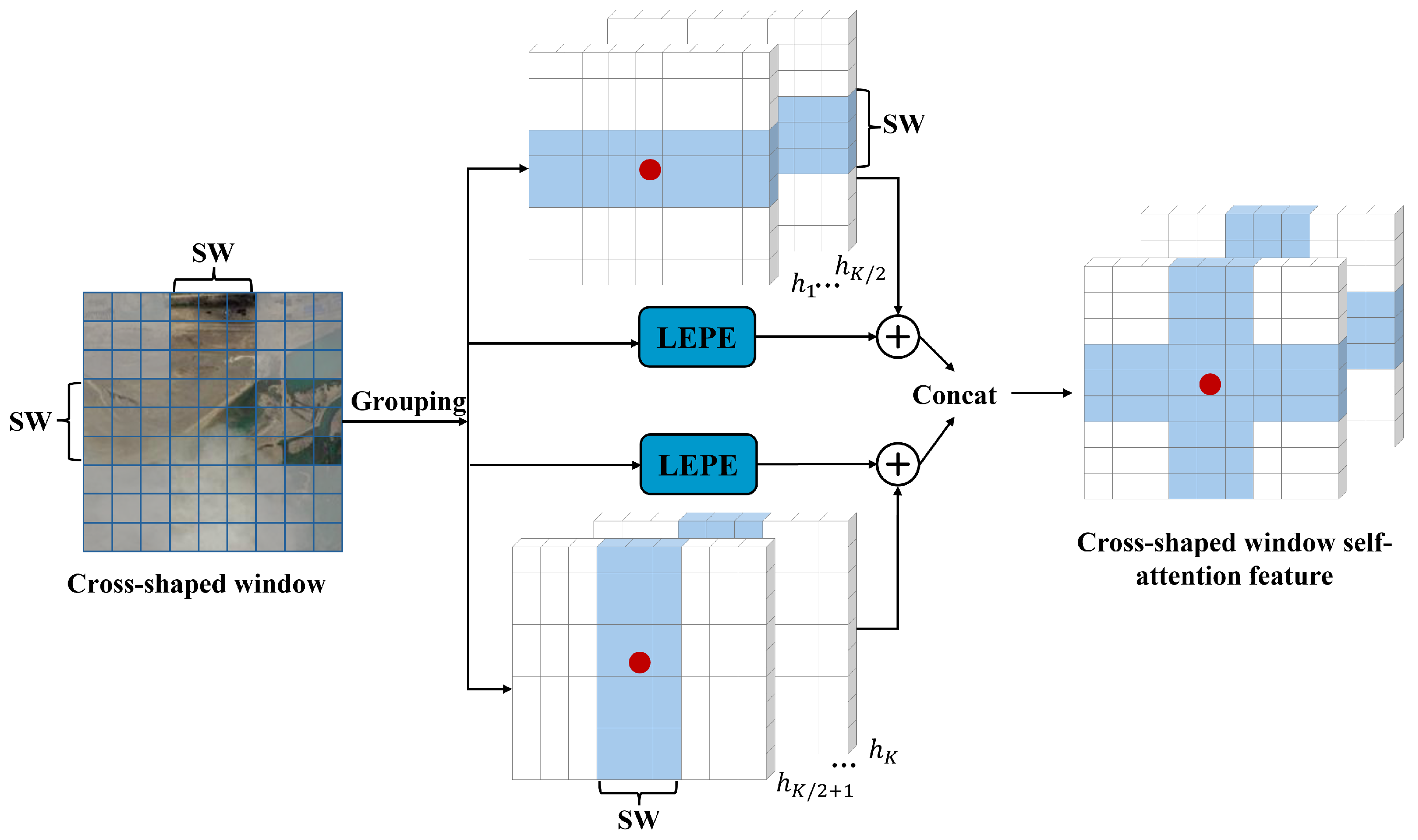Based on PVT, Swin Transformer proposed a window attention mechanism by means of a sliding window, and the computational complexity is reduced from a quadratic relationship with the size of the input image to a linear one [36]. The CSWin Transformer, building upon the Swin Transformer, replaces the window-based self-attention mechanism with a cross-shaped window attention mechanism. Additionally, it employs convolutional operations for the embedding of image patches, which brings about certain improvements and novel features in its architecture [46]. As is evident from Table 8, the segmentation precision of clouds for the model presented in this study surpasses that of the Transformer model.

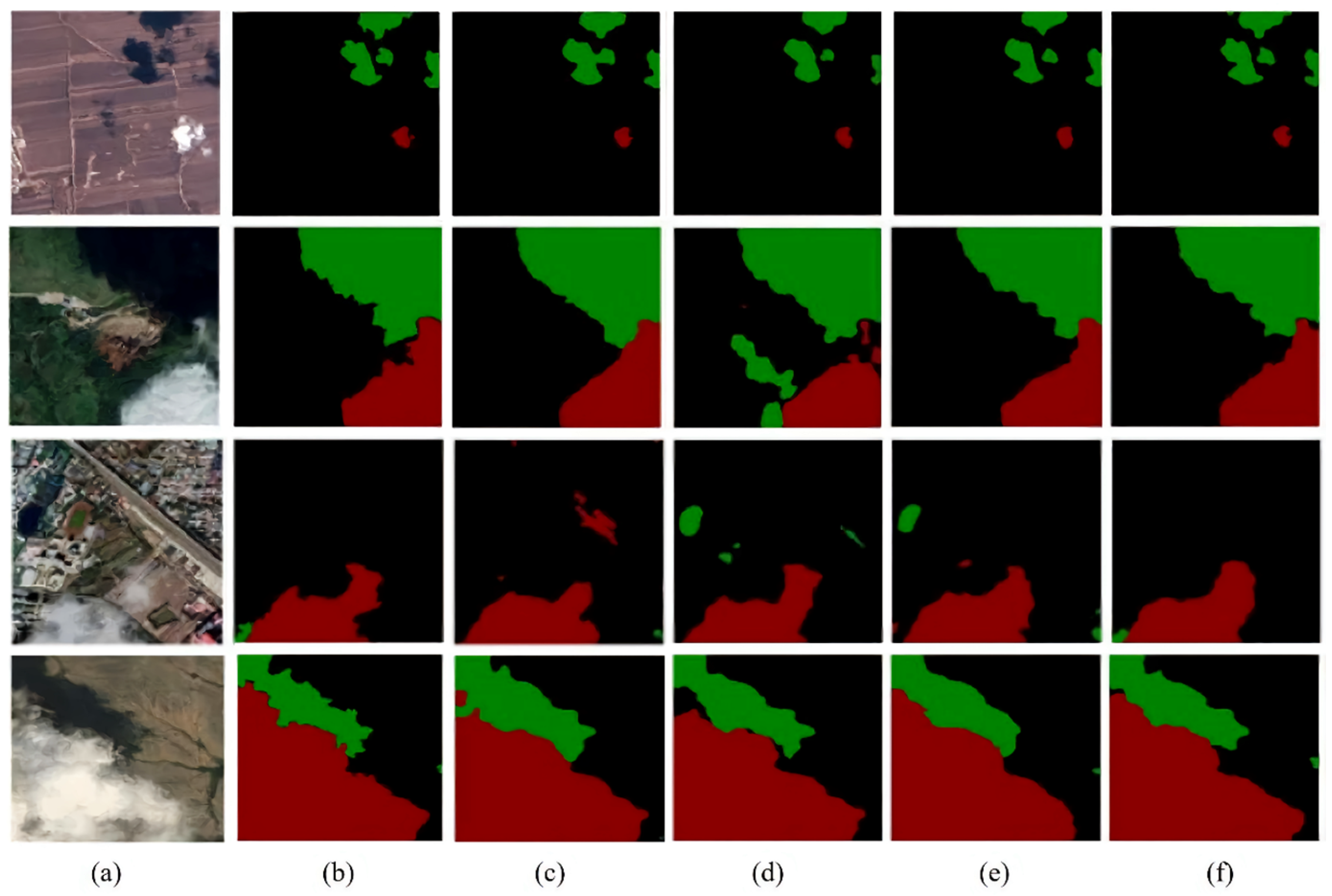
Figure 10 shows the comparative segmentation of the above model, where red, green, and black represent clouds, cloud shadows, and backgrounds, respectively. As can be seen from the cloud shadows marked in the white box in Figure 10c, the segmenter segmentation is rough and the error is large, because the network of the Transformer architecture needs to be trained on a large dataset to learn the inductive bias like CNN, and our self-made Cloud and Cloud Shadow datasets of more than 2000 is not enough to train a pure Transformer model. Apart from the constraints imposed by the dataset, the segmenter’s substantial quantity of parameters and computational load pose significant challenges. Consequently, we were compelled to restrict the training to merely 32 image patches. This limitation has severely hindered the network’s performance in the intricate tasks of segmenting clouds, leading to suboptimal results and a noticeable gap in its ability to accurately distinguish between these elements. Figure 10d shows that the PVT segmentation performance is better than that of the segmenter, because the PVT adopts a pyramid architecture, which can produce progressive feature maps. The computational cost of the PVT model has been slashed, further accentuating the benefits of multi-scale feature representation. Simultaneously, with the reduction in computational complexity, the PVT model becomes feasible to adopt smaller image patches. As a result, this not only streamlines the computational process but also significantly bolsters the accuracy of segmentation, leading to more refined and accurate delineation of objects in the segmentation task. However, PVT did not recognize the cloud shadow of the white frame in Figure 10d, indicating that it is still insufficient in local expression. Although CvT takes into account some characteristics of CNN, the segmentation prediction inside the white box in Figure 10e still has a high error, because the addition of a convolution operation alone cannot fully exploit the advantages of CNN in local expression. Although Swin Transformer and CSWin Transformer further optimize the problem of large computational effort in image segmentation and detection tasks of the Transformer architecture, the segmentation effects in the white boxes in Figure 10f,g show that their ability to recognize clouds and cloud shadow boundaries and discrete and subtle cloud shadows is still limited. However, the model proposed in this study incorporates a dual-branch structure integrating CNN and Transformer. This design endows the model with the merits of both local and global feature representation capabilities. Consequently, as demonstrated in Figure 10h, its segmentation performance outshines that of previous models, presenting more accurate and detailed segmentation results.

Since the experimental model in this study adopts a dual-branch parallel network structure of CNN and Transformer, we need to consider the parameters and computation of the model due to the limitations of computer equipment. From the data in Table 8, it can be seen that CSWin Transformer can solve the problem of excessive storage of Transformer in image segmentation and take into account the segmentation accuracy, so we selected CSWin-T as the benchmark Transformer backbone of the model in this study. Figure 11 show the segmentation effects of CSWin-T, ResNet-50, and the two-stem model proposed in this study on cloud remote sensing images. The segmentation effect in the white frame in Figure 11c shows that CSWin-T is not accurate enough in terms of cloud-shadow boundary, while Figure 11d shows that ResNet-50 is prone to pixel-level misjudgment, especially in the part framed by the white frame. This is due to the fact that ResNet-50 focuses too much on local expression and cannot grasp the segmentation effect from the overall target, so it is easily disturbed by the remote sensing background. As can be seen from Figure 11e, the model in this study performs better than CSWin-T in edge and detail processing, and better than ResNet-50 in global segmentation. This finding serves as compelling evidence that the model presented in this study has effectively harnessed the complementary strengths of the CNN’s prowess in local feature representation and the Transformer’s proficiency in global feature extraction. By seamlessly integrating these two distinct yet powerful capabilities, the model has managed to strike an optimal balance between capturing fine-grained local details and comprehending the overarching context. Consequently, in the challenging realm of remote-sensing segmentation of clouds, the model has demonstrated remarkable performance. It not only accurately delineates the boundaries of clouds and their corresponding shadows but also discerns subtle variations within these elements, resulting in highly precise and reliable segmentation outcomes.

In the above, we compare the semantic segmentation methods based on the Transformer framework and evaluate their model performance and segmentation performance in cloud detection. Next, we compare and verify some common semantic segmentation models based on CNN frameworks and some dual-stem hybrid network models, and the experimental results are shown in

Table 9. Experimental results are compared with CNN-based and CNN+Transformer segmentation networks on Cloud and Cloud Shadow datasets.

Model	PA (%)	mP (%)	mR (%)	F1 (%)	MIoU (%)	FWIoU (%)
SegNet	95.58	94.32	94.79	94.55	89.74	91.60
U-Net	96.46	95.51	95.84	95.67	91.74	93.20
FCN8s	96.55	95.76	95.74	95.75	91.89	93.36
CMT	96.63	95.93	95.86	95.89	92.14	93.51
Mobile-Former	96.83	96.28	95.94	96.12	92.55	93.86
DeepLabv3+	96.85	96.09	96.18	96.14	92.59	93.91
PSPNet	96.96	96.25	96.30	96.28	92.85	94.12
HRNet	97.09	96.16	96.74	96.45	93.17	94.38
Conformer	97.15	96.46	96.64	96.55	93.35	94.48
OCRNet	97.30	96.63	96.80	96.71	93.66	94.76
Ours	97.51	96.98	96.86	96.97	94.13	95.15

. Among them, Conformer [47] and Mobile-Former [48] are both hybrid networks of CNN and Transformer in parallel, which carry out bidirectional convergence and interaction at each stage, and Mobile-Former’s CNN framework adopts the MobileNet lightweight network. CMT is a hybrid network of CNN and Transformer serial [52].

The experimental data presented in Table 9 vividly illustrate that the method proposed in this study exhibits significant superiority in cloud and cloud shadow detection within Transformer-based networks. When juxtaposed with CNN based networks and CNN+Transformer dual-branch networks, it consistently achieves the most optimal segmentation outcomes. It outperforms the others by accurately identifying and segmenting clouds and cloud shadows, highlighting its robustness and effectiveness in handling such remote-sensing-related segmentation tasks. Due to space limitations, we selected one of the three methods based on Transformer, CNN, and CNN+Transformer for comparative effect. These three methods are CSWin-T, OCRNet, and Conformer, which have the best cloud segmentation effects among the same type of methods. 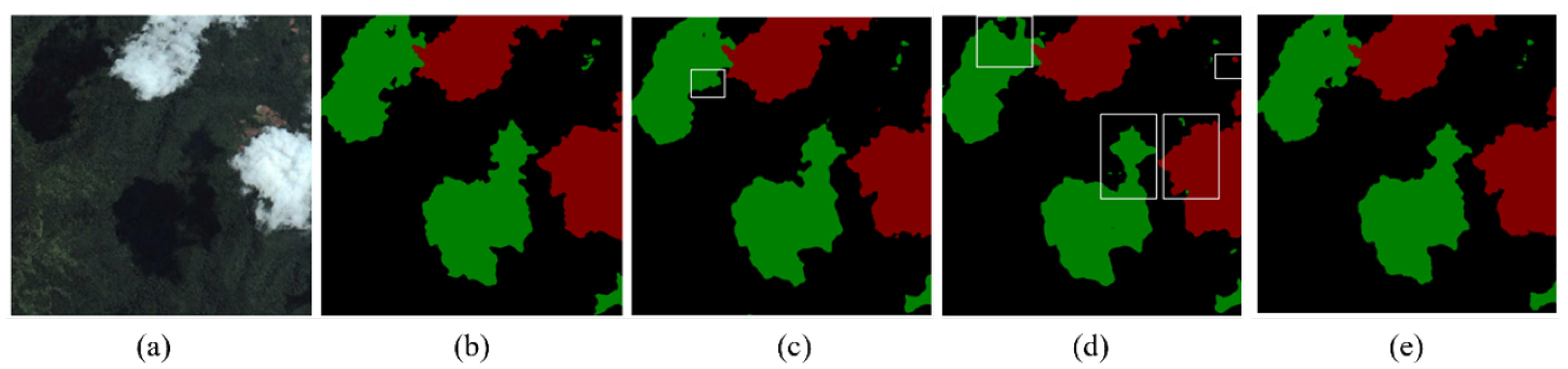Figure 12 shows the comparative segmentation of the model in this study against the complex remote sensing background.

For targets with a discrete distribution and small area, as shown in the first row of Figure 12, the model in this study has a better segmentation effect than CSWin-T. However, when the background is similar to the target, as shown in Figure 12, the dark vegetation in the second row is easy to confuse with cloud shadows, and the CNN network, such as OCRNet, is prone to misjudgment. In the case where the road and white roof are similar to clouds in the background of the towns in Figure 12 in the third row, the other three types of models have more or less mispositives, but the models in this study balance the global and local expressions, thus reducing such misjudgments. For boundary detection, as shown in Figure 12, the junction of clouds in the fourth row and their boundaries, the models in this study are better than the other three types of models. Based on the above experimental data and comparative prediction graphs, the model designed in this study shows an excellent segmentation effect on Cloud and Cloud Shadow datasets, which also verifies the effectiveness of the internal structure of the model.

3.5. Generalization Experiments

In order to assess the generalization ability of the model proposed in this study, this subsection conducts comparative experiments on two publicly accessible datasets: the HRC_WHU dataset and the SPARCS dataset.

Table 10. Experimental results with different types of segmentation networks on HRC_WHU datasets.

Model	PA (%)	mP (%)	mR (%)	F1 (%)	MIoU (%)	FWIoU (%)
Segmenter	95.21	93.52	94.70	94.10	88.94	90.96
SegNet	94.73	94.63	94.54	94.58	89.74	89.99
PVT	96.53	95.47	95.97	95.71	91.82	93.34
U-Net	95.94	95.86	95.81	95.84	92.01	92.20
HRNet	95.97	95.87	95.86	95.87	92.07	92.27
CvT	96.68	95.94	95.87	95.91	92.18	93.59
CMT	96.73	96.01	95.76	95.99	92.31	93.70
Mobile-Former	97.16	96.56	96.47	96.52	93.29	94.49
FCN8s	96.87	96.75	96.84	96.80	93.80	93.94
Swin	97.45	96.97	96.85	96.91	94.03	95.05
DeepLabv3+	97.04	96.91	97.02	96.97	94.11	94.26
CSWin	97.10	97.13	96.90	97.01	94.20	94.34
Conformer	97.19	97.09	97.16	97.12	94.41	94.54
OCRNet	97.24	97.14	97.19	97.16	94.49	94.63
PSPNet	97.25	97.16	97.21	97.18	94.53	94.65
Our	97.65	97.55	97.63	97.58	95.30	95.41

shows the experimental outcomes of various network models on the HRC_WHU dataset. Evidently, from the table, the model of this study outperforms other models in terms of recognition accuracy for the single-class cloud segmentation task. Impressively, its Mean Intersection over Union (MIoU) value reached as high as 95.30, demonstrating its superior performance and remarkable effectiveness in precisely segmenting clouds within this specific dataset.

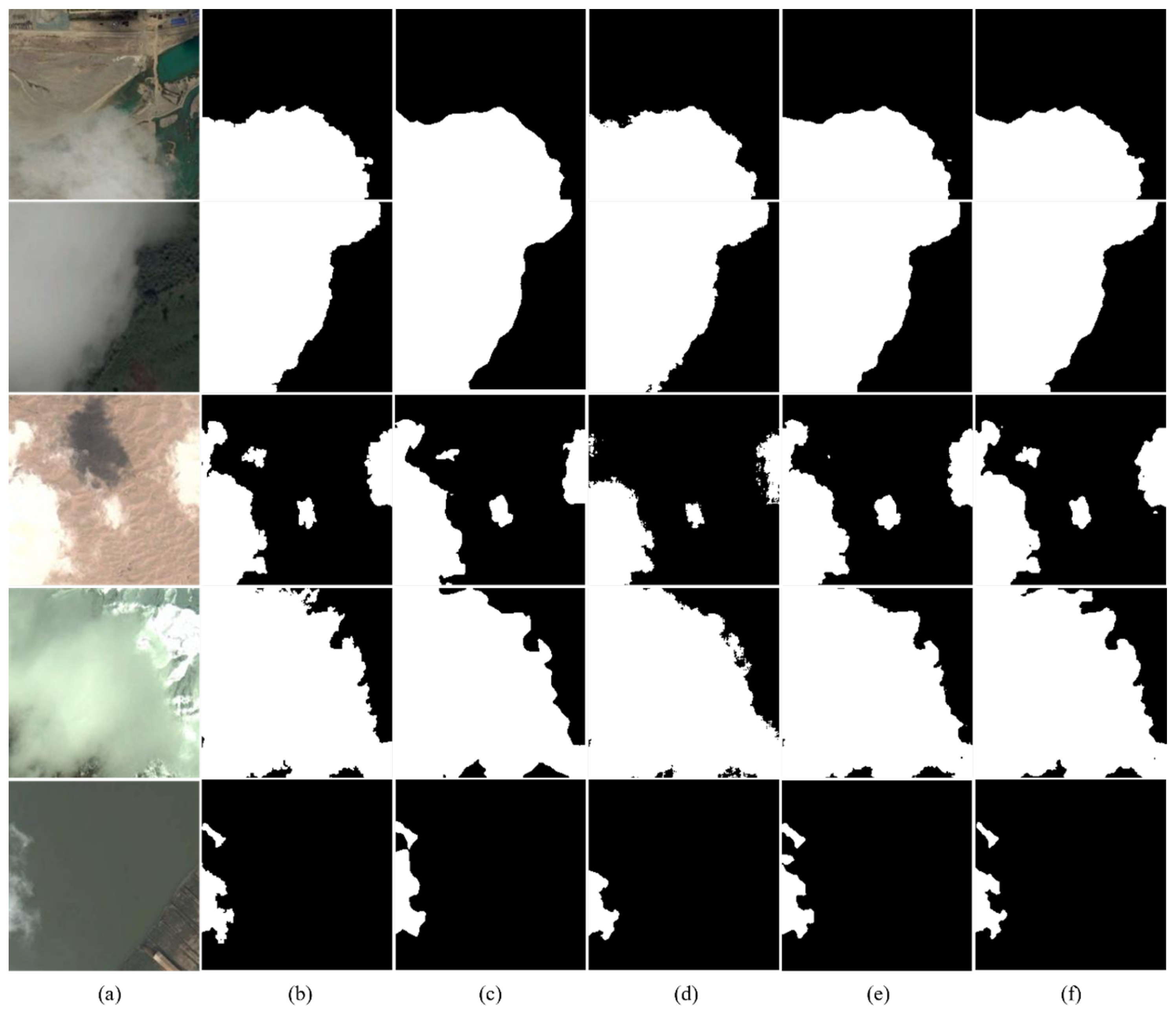
Figure 13 shows the comparative segmentation prediction plots of PSPNet, CSWin, Conformer, and the models in this study in five remote sensing backgrounds: town, vegetation, wasteland, snow, and water. Among them, the three networks compared with the models in this study are the models with the highest segmentation accuracy among the three types of networks, CNN, Transformer, and CNN+Transformer. The first and second lines of Figure 13 show that the cloud boundary recognition accuracy of this model is higher than that of the other three models. In the third and fifth rows of Figure 13, the other three models missed the smaller clouds, and our model accurately identified them. The fourth row of Figure 13 vividly reveals that in scenarios where there is a high likelihood of confusion between clouds and snow, this model significantly outperforms other models in terms of segmentation performance. It showcases remarkable resilience and accuracy, adeptly distinguishing between clouds and snow even in such challenging and ambiguous situations. This superior performance highlights the model’s robustness and effectiveness in handling complex and difficult segmentation tasks, setting it apart from its counterparts.

In order to evaluate the recognition performance of the method presented in this study for more intricate segmentation tasks, we carried out comparative experiments using the SPARCS dataset. The SPARCS dataset is a five-class classification dataset characterized by its diverse and complex remote sensing backgrounds. This richness in backgrounds provides an ideal scenario for thoroughly assessing the model’s robustness and generalization capabilities.

Table 11. Experimental results compared with different types of segmentation networks on the SPARCS dataset.

Model	PA (%)	mP (%)	mR (%)	F1 (%)	MIoU (%)	FwioU (%)
SegNet	92.19	89.46	87.64	88.48	80.07	85.80
Segmenter	92.70	91.72	89.82	90.68	83.17	86.46
PVT	94.30	92.79	92.18	92.96	86.96	89.32
PSPNet	95.56	94.02	92.81	93.39	87.84	91.61
U-Net	95.48	93.92	92.92	93.40	87.91	91.47
FCN8s	95.60	94.27	92.68	93.44	87.94	91.69
CvT	95.77	94.33	93.39	93.77	88.36	92.78
CMT	95.82	94.63	93.11	93.84	88.63	92.06
Mobile-Former	96.13	94.48	94.25	94.36	89.51	92.66
Swin	96.25	94.51	94.60	94.55	89.83	92.89
DeepLabv3+	96.43	95.21	94.16	94.67	90.05	93.18
CSWin	96.45	94.93	94.72	94.82	90.30	93.24
Conformer	96.55	95.04	94.84	94.93	90.50	93.41
HRNet	96.60	95.15	94.90	95.03	90.67	93.51
OCRNet	96.79	95.66	94.76	95.20	90.97	93.85
Our	96.91	95.81	95.03	95.45	91.35	94.10

illustrates the experimental outcomes of various network models when applied to the SPARCS dataset. The results of these experiments serve as further evidence of the outstanding performance of the model introduced in this study in the domain of remote sensing image segmentation tasks.

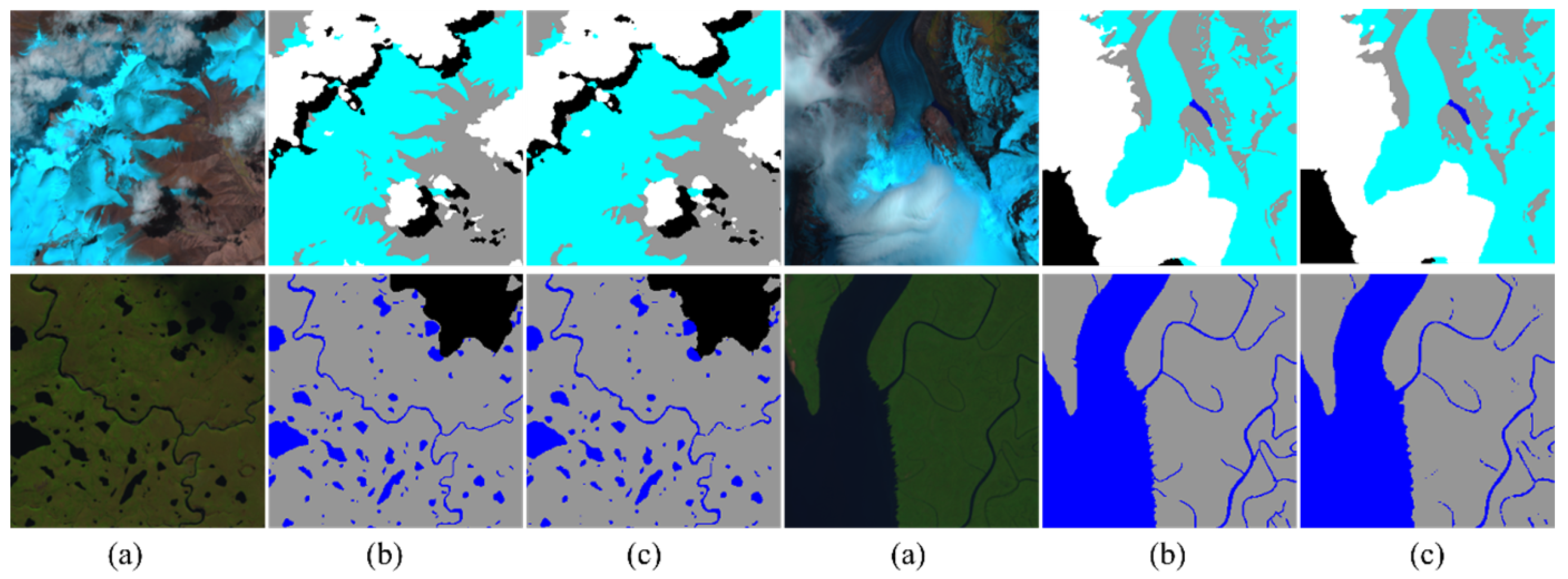
Figure 14 shows the prediction results of the model in this study for five types of segmentation tasks: clouds, cloud shadows, water, snow, and background. In the first row of the cloud and snow scene in Figure 14, the model in this study can accurately restore the complex and changeable boundaries. At the same time, in the scene of water segmentation in the second row of Figure 14, the model in this study can still have high segmentation accuracy in the face of small water areas and slender tributaries. In summary, the model in this study still achieves good segmentation results on other remote sensing datasets, which proves that the model in this study has good robustness.

3.6. Model Complexity and Performance Analysis

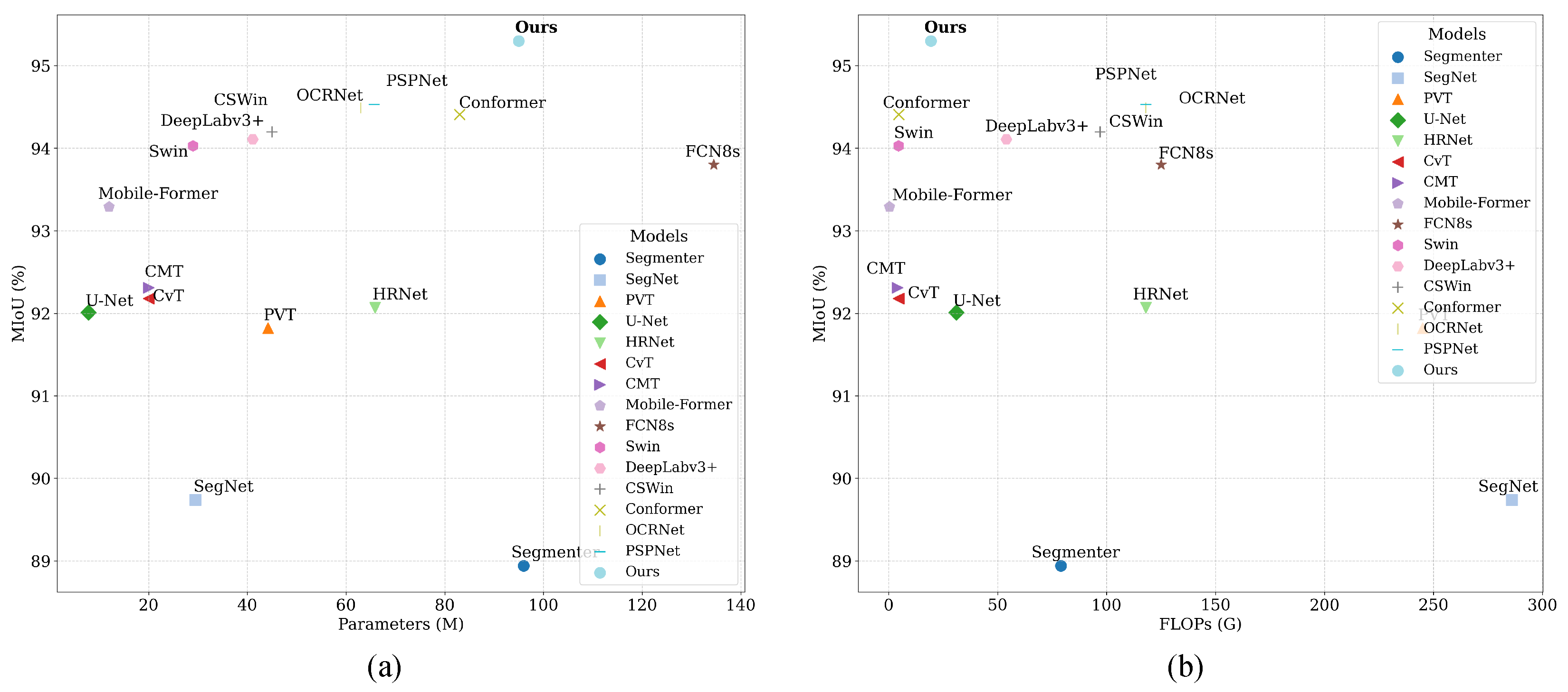
To comprehensively evaluate the efficiency and effectiveness of the proposed model, we conducted a comparative analysis of model complexity and segmentation performance across multiple representative baselines. Specifically, we considered three metrics: the number of parameters (M), the theoretical computational complexity measured by GFLOPs, and the segmentation accuracy evaluated using the mIoU (%) metric. The results are summarized on two datasets, HRC_WHU and SPARCS, as shown in Figure 15 and Figure 16.

On the HRC_WHU dataset, as shown in Figure 15, our model achieves the highest mIoU of 95.30%, while maintaining a relatively moderate parameter size of 95 M and a computational cost of 19.38 GFLOPs. Compared to models such as PSPNet and OCRNet, which achieve comparable performance (94.53% and 94.49%, respectively), our method shows a better balance between accuracy and efficiency. Notably, our FLOPs are only about 20% of that of SegNet (286 GFLOPs), and lower than most mainstream CNN+Transformer hybrid models.

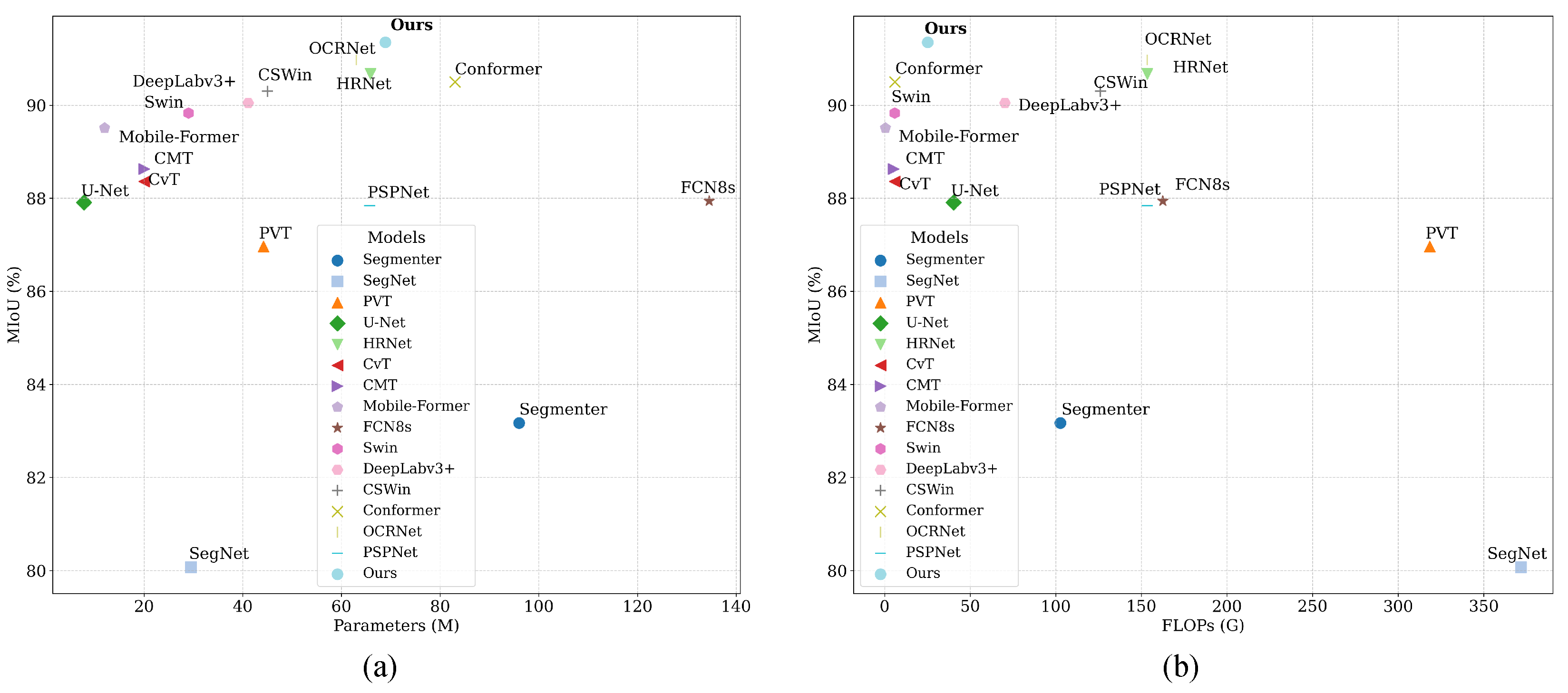
On the SPARCS dataset, with larger input dimensions (256 × 256), all models experience increased computational complexity. After adjusting FLOPs accordingly, as reported in Figure 16, our method still achieves the highest mIoU of 91.35% with only 25.19 GFLOPs. In contrast, models such as FCN8s and PVT reach lower mIoU (87.94% and 86.96%, respectively) while requiring significantly more computation (162.5 and 318.5 GFLOPs).

In both datasets, our model consistently demonstrates superior segmentation accuracy while maintaining a relatively low computational burden. This confirms the effectiveness of the dual-branch design and the lightweight feature aggregation modules in enhancing feature representation while controlling complexity.

4. Conclusions

This paper presents a novel dual-branch encoding feature aggregation network specifically designed for cloud and cloud shadow detection in remote sensing images. By integrating convolutional neural networks (CNNs) and Transformer architectures through two innovative modules—the Dual-branch Lightweight Aggregation Module (DLAM) and the Dual-branch Attention Aggregation Module (DAAM)—the proposed method effectively overcomes the limitations of existing single-backbone and naive fusion approaches. DLAM efficiently fuses shallow local and global features with low computational cost, while DAAM leverages bidirectional self-attention to facilitate deep feature interactions, significantly enhancing the model’s ability to distinguish complex cloud and cloud shadow patterns. Extensive experiments across multiple high-quality datasets demonstrate that the proposed model achieves superior segmentation accuracy and robustness compared to state-of-the-art CNN-based, Transformer-based, and hybrid networks. The ablation studies validate the effectiveness of the two-stage fusion strategy and highlight the importance of the adaptive weighting mechanisms and auxiliary supervision branches in improving training stability and generalization. Furthermore, the analysis of L2 regularization parameters provides practical insights into optimizing model convergence and performance, underscoring the methodological rigor of the proposed approach. Importantly, this work advances the field by offering a scalable and computationally efficient framework that balances local detail preservation with global context modeling, addressing a critical challenge in remote sensing cloud detection.

In future research, we plan to integrate the refined cloud and shadow masks generated by our model into downstream applications such as land cover classification, vegetation monitoring, and environmental change detection. This integration will enable a comprehensive assessment of the practical benefits and limitations of the proposed method in real-world remote sensing workflows.