A Novel Method for Estimating Parameters of Magnetic Dipole Sources Under Low Signal-to-Noise Ratio Conditions Based on LM-OBF Algorithm

Abstract

Magnetic anomaly data rapidly decay with distance and are susceptible to environmental magnetic noise, which leads to reduced accuracy and robustness in estimating magnetic source parameters. This shows significant differences between estimated and true values. Therefore, this study proposes a method for estimating magnetic source parameters based on the LM-OBF algorithm. This method transforms magnetic anomaly data into a two-dimensional orthogonal basis function space using the Gram–Schmidt orthogonalization process, establishing a new forward modeling relationship. It then constructs an objective function within a least squares framework and optimizes it using the Levenberg–Marquardt (LM) algorithm to achieve a stable estimation of magnetic source parameters. The experimental section tests this method using synthetic and field data, comparing it to traditional detection methods. The results demonstrated that the method maintains stable and accurate estimation of magnetic source parameters even at a signal-to-noise ratio (SNR) of −10 dB, outperforming traditional methods in terms of performance under strong noise interference conditions.

1. Introduction

Magnetic dipole source detection and parameter estimation, including position parameters, magnetic moment magnitude, and direction parameters, are critical issues in magnetic anomaly detection [1,2]. This technology has been extensively applied in underwater target detection [3,4], unexploded ordnance (UXO) detection [5,6], naval mine detection [7], geomagnetic assisted matching navigation [8,9], archaeology [10], and biomedical fields [11,12]. Research has demonstrated that when the distance between the target source and the measurement point exceeds 2.5 times the size of the target source, the source can be modeled as a magnetic dipole. This approximation is suitable for most “far-field” detection scenarios, such as underwater target detection and UXO detection [13,14]. With this understanding, the detection, localization, and parameter estimation of magnetic sources can be simplified to those of magnetic dipole sources. Despite magnetic anomaly detection being largely unaffected by environmental media, challenges persist, including weak target anomaly responses and complex background magnetic noise. These challenges contribute to low precision in target magnetic source localization and identification and reduce the convergence performance of optimization algorithms [15]. Addressing how to achieve high-precision localization and magnetic moment parameter inversion of target magnetic dipoles under strong noise interference remains vital in enhancing the accuracy and robustness of magnetic dipole parameter estimation.

Currently, magnetic dipole source parameter estimation is primarily divided into two parts: estimation of source position and estimation of source magnetic moment parameters. Wynn et al. [16] utilized the magnetic tensor field, independently measured by a superconducting magnetic gradiometer and an array magnetic measurement system, to determine the position of the dipole target using the eigenvector method, achieving dipole source localization. Nara et al. [17] derived a closed-form formula for the precise localization of dipole sources based on the measured magnetic gradient tensor field of the target source without the need to know the orientation of the target source. Wieger et al. [18] introduced the Scalar Triangulation And Ranging (STAR) method, which employs a cubic magnetic gradient tensor array for multi-point contraction to locate ferromagnetic targets. The STAR method facilitates immediate target localization and is unaffected by fluctuations in the Earth’s magnetic field; however, the spherical assumption of the tensor invariant introduces inherent non-spherical errors. Researchers have proposed various methods to address these errors. Lin et al. [19] proposed a STAR method that compensates for real-time direction and distance errors. However, the iterative process of the STAR method still encounters convergence difficulties in specific directions and numerical errors. Du et al. [20] proposed a robust calibration and localization method for magnetic gradient tensor measurement systems, which enhances the calibration accuracy of the magnetometer array through multi-invariant constraint calibration technology and improves the localization robustness for non-cooperative targets by adaptively selecting multiple pairs of magnetic gradient tensors combined with the Levenberg–Marquardt algorithm optimization. Clark et al. [21] introduced a source localization technique called Normalized Source Strength (NSS), based on the eigenvalues of magnetic gradient tensor data. This technique allows the localization results to be independent of the target source’s magnetization direction, enabling the unique determination of the target source’s position. Methods based on NSS have been extensively used for localizing magnetic dipole targets [22,23]. With advances in computer technology and artificial intelligence, neural networks and deep learning techniques have increasingly been applied to the localization and identification of magnetic dipole targets. Cardenas et al. [24] recognized and localized magnetic dipole target sources using a coupled network model of YOLO and DenseNet. They demonstrated the potent capabilities of artificial intelligence technology in addressing magnetic dipole source recognition and localization challenges. Miao et al. [25] employed a super-resolution deep neural network to calculate super-resolution NSS combined with an initial rough trust region reflection optimization algorithm to estimate target position parameters.

In addition to the position information of magnetic dipole sources, estimating the magnetic moment parameters of magnetic dipoles is a critical issue of interest to researchers. This estimation aids in the subsequent identification and classification of magnetic dipoles. Yin et al. [26] utilized improved tilt angles and normalized magnetic source intensity technology to estimate the position of the target source. They then employed magnetic tensor gradient data and optimization models to estimate the magnetic dipole source’s magnetic moment parameters. Ding et al. [27] combined magnetic gradient tensor data with normalized magnetic source intensity and the differential evolution (DE) algorithm to fully estimate the number, position, and magnetic moment of magnetic dipole sources. Ge et al. [28] introduced the VMGT2 angle concept, which determines the number of magnetic sources by mapping the L2 norm of the vertical magnetic gradient tensor onto the arctan function. They combined the differential evolution (DE) algorithm with the LM algorithm to optimize magnetic source parameters. Ge et al. [29] proposed a new method for the detection, localization, and classification of multiple magnetic dipole sources (DLCMMS), achieving joint parameter optimization of magnetic source number, position, and magnetic moment parameters under the cooperative co-evolution (CC) framework, with high recognition accuracy under noise-free conditions. These methods are based on magnetic gradient tensor data, and the measurement instruments are relatively complex and costly. Since the data often contains high-frequency noise and calculating the magnetic gradient tensor from scalar data involves taking unstable second-order derivatives, using scalar data to estimate the position and parameters of magnetic dipole sources is also an essential direction for magnetic source parameter estimation. Scalar measurements are often more accurate than vector and gradient tensor measurements [30]. Kolster et al. [31] proposed a recursive differential inversion combined with the Gaussian–Newton method, which can directly estimate the parameters of magnetic dipole sources without additional processing in the presence of external noise and sensor attitude changes. Wigh et al. [32] achieved parameter estimation of the ellipsoidal model and actual UXO data under the framework of probabilistic inversion using the ellipsoidal dipole model.

Despite significant advancements in magnetic dipole source parameter estimation over recent decades, few scholars have examined the accuracy and stability of these estimates under conditions of substantial interference. Improving the accuracy of magnetic dipole source parameter estimation under strong magnetic interference conditions is a vital issue for the practical application of this technology. Magnetic anomaly detection (MAD) technology primarily studies how to achieve target anomaly detection under strong noise conditions, and a variety of detection methods have been developed, including orthogonal basis decomposition, stochastic resonance, entropy filters, higher-order cross methods, and modal decomposition [33,34,35,36,37,38]. The most common method is the orthogonal basis function method (OBF) proposed by Ginzburg et al. [33] in 2002, which decomposes the magnetic anomaly data within a sliding window into three sets of orthogonal basis functions. It then uses the square sum of the function coefficients as the detection basis to achieve target anomaly detection. This method is easy to implement and highly efficient in computation, making it suitable for real-time detection applications. Wang et al. [39] extended the OBF method to two-dimensional situations using a two-dimensional sliding window. They calculated the square sum of the five independent orthogonal basis components of magnetic dipole sources under strong noise conditions as the energy function to achieve efficient magnetic anomaly detection in two-dimensional situations.

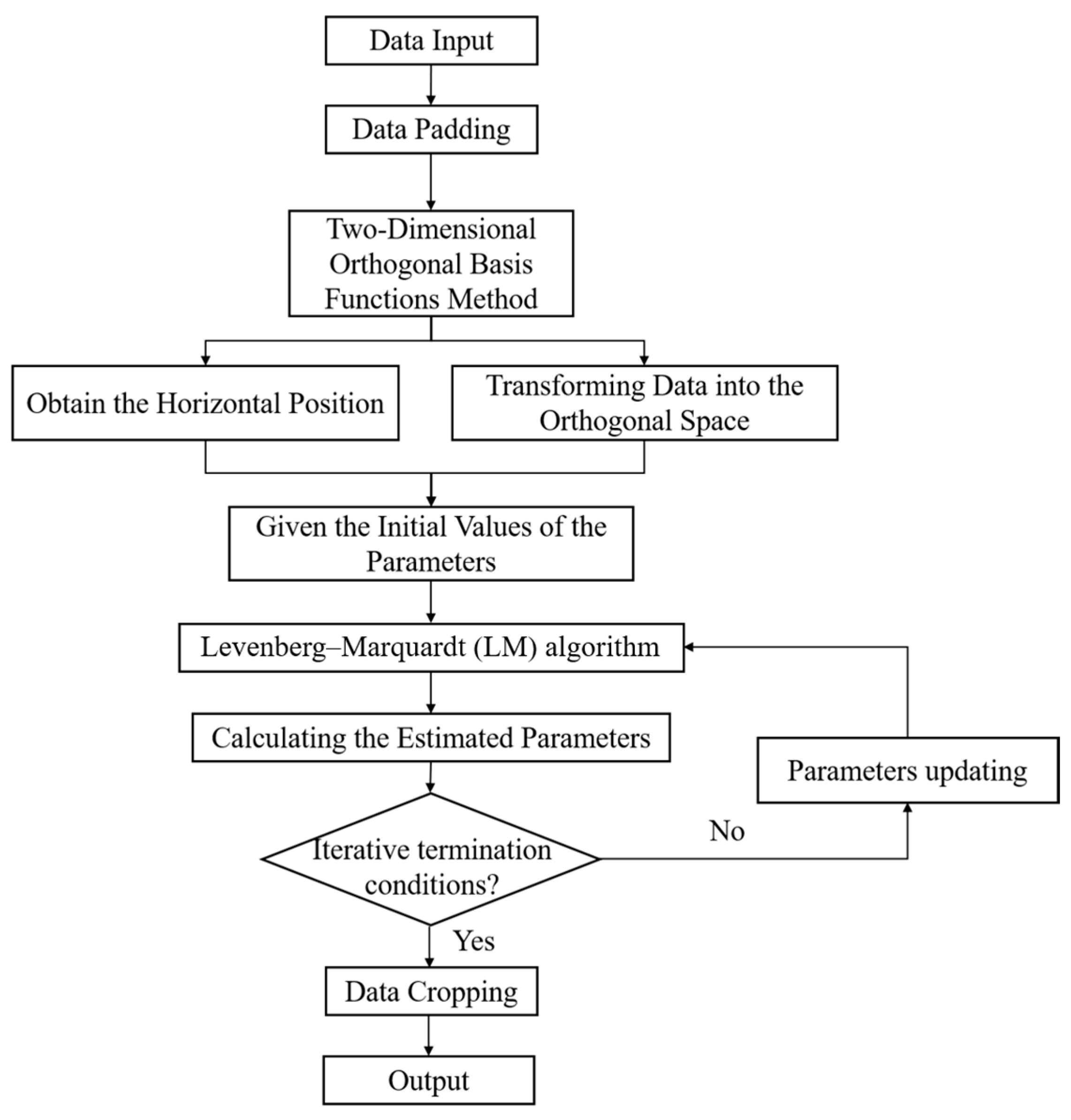
This study proposes a new method based on the LM-OBF algorithm to address the inability to estimate magnetic dipole source parameters under low SNR conditions and enhance the robustness of magnetic dipole source parameter estimation. This method transforms the measured magnetic anomaly values into orthogonal space using the Gram–Schmidt orthogonalization process, calculates the coefficient energy square sum as the forward model using orthogonal basis functions and magnetic anomaly values, and then determines the objective function required for parameter optimization within the least squares framework. Following this, the objective function is optimized using the LM algorithm to achieve accurate parameter estimation of the magnetic dipole source. The proposed method is tested on synthetic models and actual measured data, demonstrating that the LM-OBF algorithm can accurately estimate the parameters of magnetic dipole sources under low SNR conditions. This study makes several significant contributions to the field of magnetic dipole source parameter estimation: (1) It introduces a novel LM-OBF algorithm that accurately estimates the parameters of the target source directly under low SNR conditions without any denoising treatment, a rarity in previous studies. (2) It is the first to combine the OBF method with traditional optimization methods, verifying the algorithm’s effectiveness in synthetic models and actual measured data and providing new ideas for developing magnetic dipole parameter estimation methods based on other MAD methods in the future.

2. Materials and Methods

2.1. Forward Model

When the distance between a magnetic dipole source and the measurement sensor exceeds 2.5 times the size of the magnetic source, the anomaly generated by the target magnetic source can be considered characteristic of a magnetic dipole. This assumption is consistent with most “far-field” detection scenarios. In measurements involving objects such as UXO, while modeling techniques based on ellipsoidal magnetic dipoles that account for their self-demagnetization effects have significantly advanced, practical limitations remain. Specifically, the UXO’s dimensions, burial depth, and the distance between the sensor and the target cause the response from self-demagnetization effects induced by the target’s shape characteristics to attenuate with distance, complicating detection in practical applications. Therefore, the point dipole forward modeling formula sufficiently addresses most detection scenarios [40,41,42]. The response of the magnetic dipole source is expressed by the following relation [43].

$${\mathit{B}}_{\mathit{a}}={\displaystyle \frac{{\mu }_0}{4\pi }}\left({\displaystyle \frac{3\left(\mathit{m}\cdot \mathit{R}\right)\mathit{R}}{R^5}}-{\displaystyle \frac{\mathbf{m}}{R^3}}\right)$$

(1)

where ${\mu }_0$ is the permeability in free space; $\mathit{m}$ is the magnetic moment vector of the dipole, $\mathit{m}={m·\left[m_x,m_y,m_z\right]}^T$; and $\mathit{R}$ is the distance between the magnetic sensor and the target. When R $=({(x_1-x_0)}^2+{(y_1-y_0)}^2+{(z_1-z_0)}^2{)}^{1/2}$, the coordinates $x_1$, $y_1$, and $z_1$ represent the location of the observation point and $x_0$, $y_0$, and $z_0$ correspond to the position of the magnetic dipole source.

The magnetic anomalies of the target body for magnetic anomaly detection are generally much smaller than the geomagnetic field values. So the magnetic anomaly field $∆\mathrm{B}$ can be regarded as the projection of ${\mathbf{B}}_a$ in the direction of the geomagnetic field ${\mathbf{B}}_e$ when the scalar magnetic sensor is used for measurement. The formula is as follows:

$$\mathsf{\Delta }B={\displaystyle \frac{{\mathit{B}}_e\cdot {\mathit{B}}_a}{\left|{\mathit{B}}_e\right|}}=\mathbf{u}\cdot {\mathit{B}}_a$$

(2)

where $\mathbf{u}=\left(\cos \left(I\right)\cos \left(D\right)\right){\mathbf{e}}_{\mathit{x}}+\left(\cos \left(I\right)\sin \left(D\right)\right){\mathbf{e}}_{\mathit{y}}+\left(\sin \left(I\right)\right){\mathbf{e}}_{\mathit{z}}$, $D$ is the declination, and $I$ is the inclination.

In scalar magnetic measurements, the total field detected by a magnetometer generally results from the combination of the geomagnetic field and anomalous fields produced by nearby sources. These observations are typically performed within a Cartesian spatial framework where the z-axis is oriented vertically downward. The induced anomaly from a magnetic dipole target can be mathematically modeled using an established dipolar field equation [44]:

$$∆T={\displaystyle \frac{{\mu }_{0}m}{4\pi }}\sum _{n=1}^6 b_n{\phi }_n$$

(3)

where

$$\begin{gathered} {\phi }_1={\displaystyle \frac{-x^2-y^2+2z^2}{{\left[x^2+y^2+z^2\right]}^{\frac{5}{2}}}}{,\phi }_2={\displaystyle \frac{2x^2-y^2-z^2}{{\left[x^2+y^2+z^2\right]}^{\frac{5}{2}}}} \\ {\phi }_3={\displaystyle \frac{-x^2+2y^2-z^2}{{\left[x^2+y^2+z^2\right]}^{\frac{5}{2}}}},{\phi }_4={\displaystyle \frac{3xz}{{\left[x^2+y^2+z^2\right]}^{\frac{5}{2}}}} \\ {\phi }_5={\displaystyle \frac{3xy}{{\left[x^2+y^2+z^2\right]}^{\frac{5}{2}}}},{\phi }_6={\displaystyle \frac{3yz}{{\left[x^2+y^2+z^2\right]}^{\frac{5}{2}}}} \end{gathered}$$

(4)

$$\begin{array}{l}{b}_1=\sin I_0\sin I, b_2=\cos I_0\cos A_0\cos I\cos A\\ b_3=\cos I_0\sin A_0\cos \mathrm{I}\sin A\\ b_4=\sin I_0\cos I\cos A+\cos I_0\cos A_0\sin I\\ b_5=\cos I_0\sin A_0\cos I\cos A+\cos I_0\cos A_0\cos I\sin A\\ b_6=\sin I_0\cos \mathrm{I}\sin A+\cos I_0\sin A_0\sin I\end{array}$$

(5)

where $I$ and $A$ are the inclination and declination of the Earth’s magnetic field, respectively, $I_0$ and $A_0$ are the inclination and azimuth of the magnetic dipole source, as illustrated in Figure 1, and ${\mathit{m}}_{hc}$ is the projection of the magnetic dipole moment vector onto the x-y plane, with $I_0$ and $A_0$ as shown in Figure 1. $x=(x_1-x_0)$, $y=\left(y_1-y_0\right),z=(z_1-z_0)$.

The structure of ${\phi }_n$ reveals a dependency relation where φ₃ satisfies ${\phi }_3=-\left({\phi }_1+{\phi }_2\right)$, leaving the remaining five basis functions free from linear interdependence. To establish an orthogonal framework for these five independent elements within the basis set, the Gram–Schmidt method—a standard linear algebra technique for orthonormalization—can be systematically applied. Through this procedure, the five original non-orthogonal functions are transformed into an orthogonal basis, with the derived orthogonalized forms explicitly detailed in prior studies [39,45]:

$$\begin{array}{c}{f}_1\left(x,y\right)=\sqrt{{\displaystyle \frac{4z^4}{3\pi }}}{\displaystyle \frac{-x^2-y^2+2z^2}{{\left[x^2+y^2+z^2\right]}^{\frac{5}{2}}}}\\ f_2\left(x,y\right)=\sqrt{{\displaystyle \frac{32z^4}{3\pi }}}{\displaystyle \frac{3x^2-3y^2}{2{\left[x^2+y^2+z^2\right]}^{\frac{5}{2}}}}\\ f_3\left(x,y\right)=\sqrt{{\displaystyle \frac{8z^4}{3\pi }}}{\displaystyle \frac{3xz}{{\left[x^2+y^2+z^2\right]}^{\frac{5}{2}}}}\\ f_4\left(x,y\right)=\sqrt{{\displaystyle \frac{32z^4}{3\pi }}}{\displaystyle \frac{3xy}{{\left[x^2+y^2+z^2\right]}^{\frac{5}{2}}}}\\ f_5\left(x,y\right)=\sqrt{{\displaystyle \frac{8z^4}{3\pi }}}{\displaystyle \frac{3yz}{{\left[x^2+y^2+z^2\right]}^{\frac{5}{2}}}}\end{array}$$

(6)

The above basis functions satisfy the following conditions:

$$\begin{gathered} {\int }_{-\mathrm{\infty }}^{\mathrm{\infty }} {\int }_{-\mathrm{\infty }}^{\mathrm{\infty }} f_m\left(x,y\right)f_n\left(x,y\right)dxdy=0,m\ne n \\ {\int }_{-\mathrm{\infty }}^{\mathrm{\infty }} {\int }_{-\mathrm{\infty }}^{\mathrm{\infty }} f_m\left(x,y\right)f_n\left(x,y\right)dxdy=1,m=n \end{gathered}$$

(7)

The linear combination of $f_{1-5}$ can be utilized to represent the magnetic anomalies produced by any magnetic dipole source. Hence, the magnetic anomalies generated by Equation (2) can be re-expressed with the following formula:

$$\mathsf{\Delta }T\left(x,y\right)={10}^{-7}{m}_0\sum _{n=1}^5 a_n{f}_n\left(x,y\right)$$

(8)

The coefficients $a_n$ depend on the normalized parameters $I_0, { A}_0, I$, and $A$, which correlate with the projection of the magnetic anomaly $\mathsf{\Delta }T$ onto the orthogonal basis. As the orientation and location of the dipole source are unknown, $a_n$ must be derived from the inner product of $\mathsf{\Delta }T$ and the orthogonal basis functions $f_{1–5}$. In practice, $\mathsf{\Delta }T$ is discretized along the x- and y-axes. To compute this inner product, interpolation and sliding window techniques are applied. The calculation is expressed as:

$${\alpha }_n=\sum _{j=-J}^J \sum _{i=-I}^I \mathsf{\Delta }T\left(x_i,y_j\right)f_n\left(x_i,y_j\right)\mathsf{\Delta }x\mathsf{\Delta }y(n=1-5)$$

(9)

where $I$ and $J$ are the ranges of numerical integration and the dimensions of the selected sliding window, and $\mathsf{\Delta }x$ and $\mathsf{\Delta }y$ are the sizes of the grid after data gridding. The squared energy metric $E$, essential for magnetic anomaly detection (MAD), is calculated using the defined formulation. A predefined threshold is applied during MAD execution to validate anomaly detection. The two-dimensional orthogonal basis decomposition method accomplishes two tasks: (1) quantifying the number of magnetic dipole sources and (2) determining their horizontal positions by identifying the maximum $E$. This process supplies an initial horizontal position for subsequent inversion processes, thereby improving parameter estimation precision.

$$E=\sum _{i=1}^5 {\alpha }_i^2$$

(10)

Therefore, in the estimation of magnetic dipole source parameters using the LM-OBF algorithm, the forward modeling relationship for the magnetic dipole source is expressed as follows:

$$E=g\left(x_0, y_0,z_0,m,I_0,A_0\right)$$

(11)

The parameter settings of the forward model are listed in

Table 1. Parameter settings of the single magnetic dipole approximation model.

Parameter	Description	Unit
$x_0$	x coordinate	meter
$y_0$	y coordinate	meter
$z_0$	z coordinate	meter
$m$	Magnetic moment	A·m2
$I_0$	Magnetic inclination	degree
$A_0$	Azimuth	degree

.

A simulated magnetic dipole source with parameters of $x_0=2.5 \mathrm{m}, y_0=2.5 \mathrm{m}, z_0=5 \mathrm{m}$, and a magnetic moment of $10 \mathrm{A}·{\mathrm{m}}^2$ was established to illustrate the effectiveness of the forward modeling based on the two-dimensional orthogonal basis decomposition method. The Earth’s magnetic inclination is 60°, and the declination is −10°. The dipole’s inclination is 20°, and the azimuth is 30°. The spatial domain for forward modeling is a 5 × 5 m area with a grid size of 0.5 m. The forward modeling results are illustrated in Figure 2a. A noise of −5 dB was introduced into the forward modeling, and the outcomes after adding noise are displayed in Figure 2b. The formula for the SNR is as follows:

$$\mathrm{S}\mathrm{N}\mathrm{R}=10{\log }_{10}\left({\displaystyle \frac{\sum (\mathit{F}{)}^2}{\sum {\left(\widehat{\mathit{F}}-\mathit{F}\right)}^2}}\right)$$

(12)

where $\mathit{F}$ is the original signal without noise; $\widehat{\mathit{F}}$ is the noisy signal.

After the introduction of −5 dB noise, discerning any dipole source targets in the figure becomes nearly impossible, as the noise completely submerges the magnetic dipole source anomalies. Figure 3 indicates that panels (a) to (e) represent the coefficients ${\alpha }_{1–5}$, and panel (f) displays the sum of the squares of these five coefficients $E$. Figure 3f indicates that the signal location is successfully recovered after processing with the two-dimensional orthogonal basis, with the noise being almost entirely suppressed. The research and proof presented in [39] demonstrate that the energy peak and distribution of the sum of squares $E$ are only related to the horizontal position, burial depth, magnetic moment magnitude, and direction of the magnetic dipole source, forming the basis for subsequent parameter estimation.

2.2. Objective Function

The objective function assesses the discrepancy between forward modeling and the actual observed data, typically represented by the square of their difference. The residual $R_i\left(\mathit{u}\right)$ between the true observed values and the forward modeling at the $i\mathrm{t}\mathrm{h}$ sampling points can be expressed by converting the inversion problem into a least squares form as follows:

$$R_i\left(\mathit{u}\right)=F\left(\mathit{u}|g_i\left(\mathit{u}\right)-d_{obsi}\right)$$

(13)

where $d_{obsi}$ represents the actual data observed at the sampling points, $\mathit{u}=[x_0, y_0,z_0,m,I_0,A_0]$, and $F$ is the forward model.

The objective function is defined as the residual sum of squares and is established as:

$$f\left(\mathit{u}\right)={\displaystyle \frac{1}{2}}\sum _{i=1}^M \parallel F\left(\mathit{u}\right){\parallel }^2$$

(14)

where $F\left(\mathit{u}\right)$ is the normalized form of the residuals, $M$ is the total number of observation points, and $‖·‖$ is the 2-norm.

2.3. Levenberg–Marquardt Algorithm

The Taylor expansion of the objective function can be written in the following form:

$$f\left(u_k+\mathsf{\Delta }u\right)\approx f\left(u_k\right)+\mathbf{J}\left(u_k\right)\mathsf{\Delta }u$$

(15)

where $u_k$ is the solution to the nonlinear problem, $k$ is the iteration number, $\mathsf{\Delta }u$ indicates the direction of the next iteration, and $\mathbf{J}\left(u_k\right)$ is the Jacobian matrix of the residuals. The optimization problem can be expressed in the following form [46,47,48]:

$$\arg \underset{\mathsf{\Delta }u}{min} {∥f\left(u_k\right)+\mathbf{J}\left(u_k\right)\mathsf{\Delta }u∥}^2$$

(16)

The LM algorithm uses a damping factor λ to interpolate between the Gauss–Newton and gradient descent algorithms, adjusting their characteristics.

$$\arg \underset{\mathsf{\Delta }u}{min} D\left(\mathsf{\Delta }u\right)={∥f\left(u_k\right)+\mathbf{J}\left(u_k\right)\mathsf{\Delta }u∥}^2+\lambda \mathsf{\Delta }{u}^T\mathsf{\Delta }u$$

(17)

If the derivative of $\mathsf{\Delta }u$ is zero, the optimal solution can be obtained as follows:

$$\mathsf{\Delta }{u}^{*}=-{\left(\mathbf{J}\left(u_k{)}^T\mathbf{J}\right(u_k)+\lambda \mathbf{I}\right)}^{-1}\mathbf{J}(u_k{)}^{T}f\left(u_k\right)$$

(18)

Setting $\mathbf{J}\left(u_k{)}^T\mathbf{J}\right(u_k)=\mathbf{H} \mathrm{a}\mathrm{n}\mathrm{d} \mathbf{J}(u_k{)}^{T}f\left(u_k\right)=\mathbf{g}$. Then, the iteration direction of the LM algorithm can be expressed in the following form.

$$\mathsf{\Delta }u=-(\mathbf{H}+\lambda \mathbf{I}{)}^{-1}\mathbf{g}$$

(19)

The Hessian matrix $\mathbf{H}$ in the LM algorithm is constructed using the Jacobian matrix $\mathbf{J}$ of the residual vector $R_i\left(\mathit{u}\right)$. In addition, the identity matrix $\mathbf{I}$ ensures numerical stability. The ${\mathbf{J}}^T\mathbf{J}$ is the Hessian matrix, and λ is a scalar damping factor. The matrix $\mathbf{H}+\lambda \mathbf{I}$ becomes invertible due to the value of λ, which influences the step size and direction of iteration. The calculation of (${\mathbf{J}}^T\mathbf{J}$) avoids the need to compute any second-order derivatives of the residuals. The value of λ ensures that the matrix $\mathbf{H}+\lambda \mathbf{I}$ is invertible and impacts the step length and iteration direction.

The value of the damping factor λ can be updated based on the gain ratio $\rho$, which characterizes the similarity between the first-order Taylor expansion approximation and the true function, to obtain a suitable iteration direction and step length. When the gain ratio is high, indicating that the current direction of change, $\mathsf{\Delta }u$, is optimal, it is necessary to reduce λ appropriately to increase the step length, improving the convergence rate. If the gain ratio is low, a new iteration direction is required, and λ should be increased to reduce the step length until the optimal descent direction is found.

$$\rho ={\displaystyle \frac{{∥f\left(u_k\right)∥}^2-{∥f\left(u_k+\mathsf{\Delta }u\right)∥}^2}{{∥f\left(u_k\right)∥}^2-{∥f\left(u_k\right)+\mathbf{J}\left(u_k\right)\mathsf{\Delta }u∥}^2}}$$

(20)

Figure 4 depicts the flowchart of the LM-OBF algorithm, where boundary effects are initially mitigated by performing edge expansion on the input data. Then, a two-dimensional orthogonal basis decomposition is conducted to obtain the coefficient square sum energy $E$ as the forward modeling equation. The horizontal position of the magnetic dipole source is calculated based on the energy peak of $E$. After setting the initial values of the parameters, the LM algorithm updates the parameters. Once the iterative termination conditions of the optimization algorithm are met, the final results of the parameter estimation are output, achieving the parameter estimation of the magnetic dipole source.

3. Synthetic Test

3.1. Single Magnetic Dipole Source Model

This study employed the single magnetic dipole source model presented in Section 2, $x_0=2.5 \mathrm{m}, y_0=2.5 \mathrm{m}, z_0=5 \mathrm{m}$, and a magnetic moment of $10 \mathrm{A}·{\mathrm{m}}^2$ to assess the capability of the LM-OBF algorithm in estimating the parameters of a magnetic dipole source under strong background noise conditions. The Earth’s magnetic inclination is 60°, and the declination is −10°. The dipole’s inclination is 20°, and the azimuth is 30°. The spatial domain for forward modeling spans a 5 × 5 m area with a grid size of 0.5 m. Gaussian random noise ranging from 10% to 97% is introduced, resulting in a SNR varying from 10 to −15 dB to test the LM-OBF algorithm’s noise resistance in parameter estimation under different SNR conditions. For the initial values of the LM algorithm, the initial horizontal position is determined by the maximum value of $E$, the burial depth $z_0$ is set to 1 m to ensure the stability of the forward modeling and optimization process, and the initial values for the dipole’s inclination and azimuth are both set to 0. The results of the parameter estimation are shown in

Table 2. Parameter optimization errors of a single magnetic dipole source under various SNR conditions.

SNR	${\mathit{x}}_0$	${\mathit{y}}_0$	${\mathit{z}}_0$	$\mathit{m}$	${\mathit{I}}_0$	${\mathit{A}}_0$
10 dB	0.0029	0.0016	0.0243	0.0320	0.242	0.424
5 dB	0.0059	0.0047	0.0305	0.0657	0.522	0.510
0 dB	0.0126	0.0114	0.0312	0.1205	−0.654	0.675
−5 dB	0.0124	0.0153	0.0315	0.1704	−0.676	−1.530
−10 dB	0.0215	0.0182	0.0498	0.3716	−1.085	−0.261
−15 dB	0.0258	0.0415	0.0731	0.8203	−6.328	−8.907

, which displays the differences between each parameter estimated by the LM-OBF method under various SNR conditions and their true values.

When the SNR is −15 dB, the LM-OBF algorithm effectively recovers the position of the magnetic dipole source, although there are significant errors in estimating the magnitude and direction of the magnetic moment. As the SNR of the data increases, the accuracy of parameter estimation by the LM-OBF algorithm also gradually improves. At an SNR of −10 dB, the algorithm is already capable of accurately recovering the parameters of the magnetic dipole source, with the positional parameter estimation error being less than 2% and the errors in the magnitude and direction of the magnetic moment being less than 5%. These tests demonstrate the LM-OBF algorithm’s strong capabilities in estimating magnetic dipole parameters under low SNR conditions.

The data with an SNR of −10 dB is considered an example to demonstrate the effectiveness of the LM-OBF algorithm. Figure 5a represents the original magnetic dipole, Figure 5c shows the distribution of the energy function $E$ without noise, and Figure 5b,d display the noisy magnetic dipole data and its energy function $E$ distribution after noise addition, respectively. Figure 5e illustrates the energy function $E$ estimated using the LM-OBF algorithm for parameter recovery, and Figure 5f shows the residuals of the parameter estimation.

3.2. Multiple Magnetic Dipole Sources Model

In cases where multiple magnetic dipole sources exist within a region, the LM-OBF algorithm employs a strategy that begins with a two-dimensional orthogonal basis decomposition method to detect the magnetic dipoles present in the area. Once detected, these dipoles are cropped using a windowing approach and inverted individually rather than simultaneously. Three different types of dipoles were generated within a 100 × 100 m area, with parameter settings as listed in

Table 3. Parameter settings for the multiple magnetic dipole model.

Dipole	${\mathit{x}}_0$	${\mathit{y}}_0$	${\mathit{z}}_0$	$\mathit{m}$	${\mathit{I}}_0$	${\mathit{A}}_0$
Dipole I	25	25	4	8	20	30
Dipole II	50	50	5	10	60	−10
Dipole III	75	75	5	10	0	0

to evaluate the LM-OBF algorithm’s capability in estimating parameters of multiple magnetic dipoles.

Table 4. Parameter optimization errors of Magnetic Dipole I under various SNR conditions.

SNR	${\mathit{x}}_0$	${\mathit{y}}_0$	${\mathit{z}}_0$	$\mathit{m}$	${\mathit{I}}_0$	${\mathit{A}}_0$
10 dB	0.0031	0.0027	0.0040	0.0285	0.2651	0.5124
5 dB	0.0062	0.0053	0.0085	0.0521	0.5332	0.7023
0 dB	0.0123	0.0101	0.0182	0.1223	0.7012	0.8524
−5 dB	0.0189	0.0168	0.0345	0.2103	0.8734	1.2345
−10 dB	0.0313	0.0232	0.0857	0.3421	2.0243	1.6342
−15 dB	0.0301	0.0355	0.0678	0.5623	4.3456	6.1234

,

Table 5. Parameter optimization errors of Magnetic Dipole II under various SNR conditions.

SNR	${\mathit{x}}_0$	${\mathit{y}}_0$	${\mathit{z}}_0$	$\mathit{m}$	${\mathit{I}}_0$	${\mathit{A}}_0$
10 dB	0.0042	0.0035	0.0061	0.0345	0.2854	0.6242
5 dB	0.0078	0.0069	0.0102	0.0624	0.6215	0.8431
0 dB	0.0154	0.0143	0.0228	0.1456	0.8231	1.0542
−5 dB	0.0231	0.0206	0.0423	0.2643	1.0453	1.4562
−10 dB	0.0283	0.0251	0.0546	0.3725	1.2045	1.8531
−15 dB	0.0372	0.0403	0.0724	0.6789	3.5342	4.3645

and

Table 6. Parameter optimization errors of Magnetic Dipole III under various SNR conditions.

SNR	${\mathit{x}}_0$	${\mathit{y}}_0$	${\mathit{z}}_0$	$\mathit{m}$	${\mathit{I}}_0$	${\mathit{A}}_0$
10 dB	0.0053	0.0041	0.0074	0.0412	0.3156	0.7341
5 dB	0.0089	0.0075	0.0121	0.0753	0.6543	0.9642
0 dB	0.0176	0.0152	0.0246	0.1672	0.9124	1.1245
−5 dB	0.0257	0.0215	0.0481	0.2941	1.1054	1.6324
−10 dB	0.0325	0.0293	0.0607	0.4012	1.3845	2.0432
−15 dB	0.1023	0.0932	0.1225	0.7341	4.7456	4.5463

present the parameter estimation errors for three magnetic dipole sources under SNR ranging from 10 dB to −15 dB. These results demonstrate the LM-OBF algorithm’s ability to estimate parameters for data containing multiple magnetic dipole sources.

Figure 6a depicts the original magnetic dipole sources, Figure 6c shows the distribution of the energy function E without noise, and Figure 6b,d display the noisy magnetic dipole data and its corresponding energy function $E$ distribution after noise addition, respectively. Figure 5e illustrates the energy function $E$ estimated using the LM-OBF algorithm for parameter recovery, and Figure 6f shows the fit residuals from the parameter estimation.

3.3. Method Comparison

The traditional LM algorithm and the NMLM algorithm proposed in this study are compared to determine the effectiveness of the LM-OBF method in estimating magnetic dipole parameters under strong noise interference conditions [48]. The NMLM algorithm introduces a new method for calculating the damping factor by analyzing the impact of noise on higher-order and lower-order matrices, which significantly improves the adaptability of the LM algorithm to noise.

Monte Carlo simulations were employed to conduct 300 parameter estimation experiments under various SNR conditions using different parameter estimation methods. Figure 7, Figure 8, Figure 9 and Figure 10 illustrate the average estimation errors of different parameters for the LM, NMLM, and LM-OBF methods under different SNR conditions. In the SNR range from −10 to 0 dB, due to the low SNR, the LM and NMLM methods either failed to converge or exhibited large estimation errors; thus, the results are not displayed. Under SNR conditions from 5 to 10 dB, the LM-OBF algorithm’s parameter estimation significantly outperformed both the LM and NMLM methods. Comparative experimental results indicate that the proposed LM-OBF method is capable of stable and accurate parameter estimation for magnetic dipole sources under low SNR conditions.

4. Field Data Test

The experiment was conducted at a site in Changchun City, Jilin Province, China, with the test area covering 12 × 11 m. This experiment simulated a realistic measurement scenario of unexploded ordnance (UXO) targets using an unmanned aerial vehicle (UAV) magnetic survey system. The magnetic measurement platform utilized was a multi-rotor airborne magnetic survey system, and the flight platform was a DJI M300 RTK multi-rotor UAV designed for autonomous flight along a pre-planned flight path with enhanced flight stability. The measurement instrument was a compact, high-precision rubidium optically pumped scalar magnetometer with a maximum sampling rate of 10 Hz. The UXO target consisted of a safely deactivated 122 mm caliber artillery shell casing buried at a depth of approximately 0.7 m to simulate an actual measurement site. The UAV magnetic survey system maintained a flight height of 1 m, a flight speed of 1 m/s, and a line spacing of 1 m, and the sampling rate of the magnetometer was set at 10 Hz to ensure high data quality. Figure 11 illustrates a schematic of the UXO target and the raw magnetic anomalies measured without processing (the actual coordinates have been replaced by distances).

Figure 12 depicts the schematic diagram of the UAV aerial magnetic system and the simulated UXO target. The measured magnetic anomalies were processed to isolate the magnetic anomalies attributable only to the target. Utilizing the International Geomagnetic Reference Field (IGRF), the local normal geomagnetic field was calculated at 55,148 nT. The team subtracted this normal field value from the measurement data to eliminate the geomagnetic background field. In addition, they subtracted the mean value of the data to ensure that the average baseline of the anomaly data was zero. The processed data are displayed in Figure 13.

Table 7. Known parameters of the artillery shell target.

Target	${\mathit{x}}_0$	${\mathit{y}}_0$	${\mathit{z}}_0$	$\mathit{m}$	${\mathit{I}}_0$	${\mathit{A}}_0$
122 mm projectile	6.5	7	0.7	/	/	/

provides the known parameter information of the artillery shell target, while

Table 8. Parameter estimation results of different methods.

Method	${\mathit{x}}_0$	${\mathit{y}}_0$	${\mathit{z}}_0$	$\mathit{m}$	${\mathit{I}}_0$	${\mathit{A}}_0$
LM	6.75	6.54	1.52	5.725	1.25	−50.26
NMLM	6.85	7.12	1.08	5.650	0.26	−60.32
LM-OBF	6.53	7.06	0.83	4.835	−10.96	99.03

compares the parameter estimation results of the LM-OBF method to two other ones. The parameter estimation results demonstrate that the LM-OBF algorithm showed superior performance in the presence of specific noise levels and aligns well with the known information.

Figure 14 further validates the parameter estimation effectiveness of the LM-OBF method on actual measured data. Figure 14a displays the processed raw anomalies, Figure 14b shows the original anomaly energy E after two-dimensional OBF processing, Figure 14c presents the restored energy E from the parameter estimation results, and Figure 14d illustrates the residuals of the parameter estimation. The application of field data underscores that the LM-OBF method exhibits robust adaptability to actual noisy data and provides superior parameter estimation results compared to traditional methods.

It is worth noting that to accurately compare the precision of different methods, a more appropriate target would be a small point-like magnetic dipole. We are planning to perform an appropriate field test later on.

5. Discussion

Magnetic dipole source parameter estimation is critical in magnetic anomaly detection and identification. However, traditional methods for estimating magnetic source parameters do not achieve stable and accurate estimations under low SNR conditions, which significantly hampers the practical application of these methods. This study introduces a novel method for magnetic source parameter estimation based on the LM-OBF algorithm, which can accurately estimate the parameters of magnetic dipole sources under low SNR conditions (down to −10 dB), providing an innovative strategy for magnetic source parameter estimation in such scenarios.

Although the LM-OBF algorithm enhances the accuracy and stability of traditional methods in the presence of strong noise interference, it has certain limitations. First, the LM-OBF algorithm depends on the results of two-dimensional OBF decomposition. The OBF method exhibits weaker noise suppression capability for mixed noise of granular and Gaussian noise and for colored noise, which are almost inevitable in complex real-world measurement environments. This reduction undoubtedly decreases the parameter estimation accuracy of the LM-OBF algorithm. Therefore, in practical measurement environments, it is essential to avoid such noise sources as much as possible. Simultaneously, future research should focus on noise reduction techniques such as autoregressive techniques and Kalman filtering to further filter out or whiten the noise, enhancing the practical performance of the LM-OBF algorithm. The tests were conducted on a computer equipped with an Intel Xeon Bronze 3204 CPU @ 1.90 GHz and 128 GB RAM. For a 50 × 50 grid (2500 data points), the parameter inversion process required approximately 5.5 min to complete. The computation time increases significantly with larger datasets, and under high-noise conditions, the inversion algorithm may require extended iterations to adequately fit the observed data. To enhance computational efficiency, future work could explore GPU parallelization strategies or distributed computing frameworks to expand the applicability of the LM-OBF method in large-scale detection tasks.

The practical deployment of UAV-based magnetic inversion inherently involves trade-offs between theoretical precision and real-world operational constraints. A critical factor is the positioning accuracy of the Real-Time Kinematic (RTK) system, which provides centimeter-level horizontal precision (±1 cm + 1 ppm) and sub-decimeter vertical accuracy (±0.1 m under stable conditions). While this meets the requirements for most near-surface magnetic surveys, residual errors arising from UAV attitude fluctuations or transient signal loss can introduce minor but non-negligible offsets in sensor positioning. These deviations were mitigated through post-processing gridding.

Height-dependent anomalies further complicate inversion accuracy. Variations in UAV altitude—even within the RTK’s specified tolerance—alter the magnitude and spatial distribution of the target’s magnetic signature. For instance, a vertical drift of 10 cm at a flight height of 1 m can induce a ~5–10% change in anomaly amplitude for a shallow dipole source. To address this, our workflow assumes a constant elevation plane during gridding, effectively averaging altitude-related variations. However, this approximation becomes less reliable in highly undulating terrains or for deeply buried targets, where altitude errors disproportionately amplify depth estimation uncertainties.

In addition, the LM-OBF algorithm utilizes the traditional LM method, which encounters specific issues concerning iteration speed and global convergence properties. When processing small datasets, the LM-OBF algorithm can reach the optimal solution within a relatively short number of iterations and time. However, with the increase in data volume, such as in the case of large-area data or under dense sampling conditions, the LM-OBF algorithm faces prolonged iteration times. This limitation constrains the application of the LM-OBF algorithm to the post-processing and identification stages of data, making it unsuitable for real-time parameter estimation scenarios involving magnetic dipole sources.

In addition, the accuracy of magnetic anomaly data itself significantly influences the LM-OBF algorithm’s accuracy in estimating the parameters of magnetic dipole sources. For example, the data obtained during total field scalar measurements includes the superimposed anomalies of the geomagnetic background field and the target magnetic source. Accurately separating the target magnetic anomaly from the geomagnetic background anomaly, ensuring that the data contains only the magnetic anomalies generated by the target magnetic source, will profoundly affect parameter estimation accuracy under actual measurement conditions. This separation can lead to significant deviations between the actual and estimated values. Therefore, developing more accurate field separation strategies or investigating parameter estimation methods based on gradient and tensor data will hold greater practical significance in the future.

6. Conclusions

This study proposes a method using the LM-OBF approach in response to the limited accuracy and robustness of magnetic source parameter estimation under strong background noise conditions. This method combines magnetic anomaly detection techniques with conventional parameter optimization algorithms, establishing a novel forward modeling relationship. It transforms magnetic anomaly data into a two-dimensional orthogonal basis function space through the Gram–Schmidt orthogonalization process. An objective function is then constructed within a least squares framework and optimized using the LM algorithm, achieving a stable estimation of magnetic source parameters. Results from synthetic models and field experiments demonstrated that the LM-OBF algorithm can accurately and stably estimate the position, magnitude of magnetic moment, and directional parameters of magnetic dipoles, even under a minimum signal-to-noise ratio of −10 dB. However, this method still encounters several challenges in practical applications: (1) The OBFs method shows limited adaptability to non-Gaussian noise, potentially reducing the effectiveness of LM-OBF parameter estimation in complex real-world noise environments. (2) The parameter estimation speed of the LM-OBF algorithm is slow for large-scale data, making it unsuitable for scenarios requiring real-time estimation. (3) Effectively isolating the magnetic target source from the background field to ensure that the inversion data contains only the target magnetic anomalies is crucial for accurate parameter estimation. Addressing these issues is critical to further advancing magnetic source parameter estimation under strong noise interference.

References

1. Liu, H.; Zhang, X.; Dong, H.; Liu, Z.; Hu, X. Theories, applications, and expectations for magnetic anomaly detection technology: A review. IEEE Sens. J. 2023, 23, 17868–17882. [Google Scholar] [CrossRef]
2. Zhao, Y.; Zhang, J.H.; Li, J.H.; Liu, S.; Miao, P.X.; Shi, Y.C.; Zhao, E.M. A brief review of magnetic anomaly detection. Meas. Sci. Technol. 2020, 32, 042002. [Google Scholar] [CrossRef]
3. Shan, Z.; Zheng, X.; Li, D.; Lu, R. Research on optimization selection of anti-submarine aircraft course in aero-magnetic exploration. Zhihui Kongzhi Yu Fangzhen 2023, 42, 76–81. [Google Scholar]
4. Zhang, Y.Q.; Wang, G.-Y. Anti-submarine patrol aircraft’s responding-antisubmarine effectiveness model research by using magnetic finder. In Proceedings of the International Congress on Industrial and Applied Mathematics, Beijing, China, 10–14 August 2015; pp. 907–910. [Google Scholar]
5. Sanchez, V.; Li, Y.; Nabighian, M.N.; Wright, D.L. Numerical modeling of higher order magnetic moments in UXO discrimination. IEEE Trans. Geosci. Remote Sens. 2008, 46, 2568–2583. [Google Scholar] [CrossRef]
6. Zalevsky, Z.; Bregman, Y.; Salomonski, N.; Zafrir, H. Resolution enhanced magnetic sensing system for wide coverage real time UXO detection. J. Appl. Geophys. 2012, 84, 70–76. [Google Scholar] [CrossRef]
7. Qin, T.; Zhou, L.; Chen, S.; Chen, Z. The novel method of magnetic anomaly recognition based on the fourth order aperiodic stochastic resonance. IEEE Sens. J. 2022, 22, 17043–17053. [Google Scholar] [CrossRef]
8. Chen, Z.; Zhang, Q.; Pan, M.; Chen, D.; Wan, C.; Wu, F.; Liu, Y. A New Geomagnetic Matching Navigation Method Based on Multidimensional Vector Elements of Earth’s Magnetic Field. IEEE Geosci. Remote Sens. Lett. 2018, 15, 1289–1293. [Google Scholar] [CrossRef]
9. Kang, C.; Wang, M.; Fan, L.M.; Zhang, X.J. Region selected of geomagnetic-matching navigation based on geomagnetic entropy and geomagnetic variance entropy. Yingyong Jichu Yu Gongcheng Kexue Xuebao/J. Basic Sci. Eng. 2015, 23, 1156–1165. [Google Scholar]
10. Accomando, F.; Florio, G. Drone-Borne Magnetic Gradiometry in Archaeological Applications. Sensors 2024, 24, 4270. [Google Scholar] [CrossRef]
11. Liu, X.; Han, J.; Xiao, W.; Wu, T.; Peng, X.; Guo, H. Magnetic field imaging with radio-frequency optically pumped magnetometers [Invited]. Chin. Opt. Lett. 2024, 22, 60006. [Google Scholar] [CrossRef]
12. Göksu, C.; Gregersen, F.; Scheffler, K.; Eroğlu, H.H.; Heule, R.; Siebner, H.R.; Hanson, L.G.; Thielscher, A. Volumetric measurements of weak current–induced magnetic fields in the human brain at high resolution. Magn. Reson. Med. 2023, 90, 1874–1888. [Google Scholar] [CrossRef] [PubMed]
13. Chen, M.; Pan, Z. Adaptive detecting algorithm for magnetic anomaly signal. Chin. J. Sens. Actuators 2014, 27, 916–921. [Google Scholar]
14. Hinze, W.J.; Von Frese, R.R.; Von Frese, R.; Saad, A.H. Gravity and Magnetic Exploration: Principles, Practices, and Applications, 1st ed.; Cambridge University Press: Cambridge, UK, 2013. [Google Scholar] [CrossRef]
15. Zhao, J.-W.; Zeng, Z.-F.; Zhou, S.; Yan, J.-H.; Guo, H.; Jia, H.-F.; Jiao, J.; Zeng, X.-C. A Fully Parameter Adaptive Magnetic Anomaly Detection Method Based on Multistable Stochastic Resonance System. IEEE Trans. Instrum. Meas. 2024, 73, 1–13. [Google Scholar] [CrossRef]
16. Wynn, W.; Frahm, C.; Carroll, P.; Clark, R.; Wellhoner, J.; Wynn, M. Advanced superconducting gradiometer/Magnetometer arrays and a novel signal processing technique. IEEE Trans. Magn. 1975, 11, 701–707. [Google Scholar] [CrossRef]
17. Nara, T.; Suzuki, S.; Ando, S. A closed-form formula for magnetic dipole localization by measurement of its magnetic field and spatial gradients. IEEE Trans. Magn. 2006, 42, 3291–3293. [Google Scholar] [CrossRef]
18. Wiegert, R.; Oeschger, J. Generalized magnetic gradient contraction based method for detection, localization and discrimination of underwater mines and unexploded ordnance. In Proceedings of the OCEANS 2005 MTS/IEEE, Washington, DC, USA, 19–23 September 2005; pp. 1325–1332. [Google Scholar]
19. Lin, S.; Pan, D.; Wang, B.; Liu, Z.; Liu, G.; Wang, L.; Li, L. Improvement and omnidirectional analysis of magnetic gradient tensor invariants method. IEEE Trans. Ind. Electron. 2021, 68, 7603–7612. [Google Scholar] [CrossRef]
20. Du, G.; Wang, Y.; Wang, G.; Chen, Q. A Robust Calibration and Adaptive Multipair of Magnetic Gradient Tensors Localization Method for Magnetic Anomaly Detection. IEEE Trans. Geosci. Remote Sens. 2023, 61, 1–14. [Google Scholar] [CrossRef]
21. Clark, D.A. New methods for interpretation of magnetic vector and gradient tensor data; I, Eigenvector analysis and the normalised source strength. Explor. Geophys. 2012, 43, 267–282. [Google Scholar] [CrossRef]
22. Yin, G.; Li, P.; Wei, Z.; Liu, G.; Yang, Z.; Zhao, L. Magnetic dipole localization and magnetic moment estimation method based on normalized source strength. J. Magn. Magn. Mater. 2020, 502, 166450. [Google Scholar] [CrossRef]
23. Yin, G.; Zhang, L.; Jiang, H.; Wei, Z.; Xie, Y. A closed-form formula for magnetic dipole localization by measurement of its magnetic field vector and magnetic gradient tensor. J. Magn. Magn. Mater. 2020, 499, 166274. [Google Scholar] [CrossRef]
24. Cárdenas, J.; Denis, C.; Mousannif, H.; Camerlynck, C.; Florsch, N. Magnetic anomalies characterization; deep learning and explainability. Comput. Geosci. 2022, 169, 105227. [Google Scholar] [CrossRef]
25. Miao, L.; Zhang, T.; Zuo, C.; Chen, Z.; Yang, X.; Ouyang, J. A Rapid Localization Method Based on Super Resolution Magnetic Array Information for Unknown Number Magnetic Sources. Sensors 2024, 24, 3226. [Google Scholar] [CrossRef] [PubMed]
26. Yin, G.; Zhang, Y.; Fan, H.; Li, Z.; Ren, G. Detection, localization and classification of multiple dipole-like magnetic sources using magnetic gradient tensor data. J. Appl. Geophys. 2016, 128, 131–139. [Google Scholar]
27. Ding, X.; Li, Y.; Luo, M.; Chen, J.; Li, Z.; Liu, H. Estimating locations and moments of multiple dipole-like magnetic sources from magnetic gradient tensor data using differential evolution. IEEE Trans. Geosci. Remote Sens. 2022, 60, 5904913. [Google Scholar] [CrossRef]
28. Ge, L.; Han, Q.; Tong, X.; Wang, Y. Detection, location, and classification of multiple dipole-like magnetic sources based on l2 norm of the vertical magnetic gradient tensor data. Sensors 2023, 23, 4440. [Google Scholar] [CrossRef]
29. Ge, L.; Han, Q.; Tong, X.; Xue, Q.; Qiao, Z. High-Resolution Detection, Localization, and Classification of Multiple Magnetic Dipole Sources. IEEE Geosci. Remote Sens. Lett. 2024, 21, 1–5. [Google Scholar] [CrossRef]
30. You, H.; Li, J.; Xu, J.; Xu, J.; Ning, T.; Gao, Y.; Li, L. A method for estimating magnetic target location by employing total field and its gradients data. Sci. Rep. 2022, 12, 17985. [Google Scholar] [CrossRef]
31. Kolster, M.E.; Døssing, A. Scalar magnetic difference inversion applied to UAV-based UXO detection. Geophys. J. Int. 2021, 224, 468–486. [Google Scholar] [CrossRef]
32. Wigh, M.D.; Hansen, T.M.; Dossing, A. Inference of unexploded ordnance (UXO) by probabilistic inversion of magnetic data. Geophys. J. Int. 2020, 220, 37–58. [Google Scholar] [CrossRef]
33. Ginzburg, B.; Frumkis, L.; Kaplan, B.-Z. Processing of magnetic scalar gradiometer signals using orthonormalized functions. Sens. Actuators A Phys. 2002, 102, 67–75. [Google Scholar] [CrossRef]
34. Sheinker, A.; Shkalim, A.; Salomonski, N.; Ginzburg, B.; Frumkis, L.; Kaplan, B.-Z. Processing of a scalar magnetometer signal contaminated by 1/fα noise. Sens. Actuators A Phys. 2007, 138, 105–111. [Google Scholar] [CrossRef]
35. Wan, C.B. Investigations on the Theory and Method of Magnetic Anomaly Detection. Ph.D. Thesis, National University of Defense Technology, Changsha, China, 2018. [Google Scholar]
36. Zheng, X.; Xu, Q.; Zhou, M.; Liu, H.; Qiu, S.; Sun, L.; Li, Q. An orthonormalized basis function algorithm based on wavelet analysis for magnetic anomaly detection. In Proceedings of the 10th International Congress on Image and Signal Processing, BioMedical Engineering and Informatics (CISP-BMEI), Shanghai, China, 14–16 October 2017; pp. 1–5. [Google Scholar]
37. Sheinker, A.; Lerner, B.; Salomonski, N.; Ginzburg, B.; Frumkis, L.; Kaplan, B. Magnetic anomaly detection using entropy filter. Meas. Sci. Technol. 2008, 19, 045205. [Google Scholar] [CrossRef]
38. Sheinker, A.; Ginzburg, B.; Salomonski, N.; Dickstein, P.A.; Frumkis, L.; Kaplan, B.-Z. Magnetic anomaly detection using high-order crossing method. IEEE Trans. Geosci. Remote Sens. 2012, 50, 1095–1103. [Google Scholar] [CrossRef]
39. Wang, T.; Li, J.; Liu, N.; Peng, S.; Li, Y.; Fang, G. A new data processing method for magnetic anomaly detection and localization based on 2-D orthonormal basis functions. IEEE Trans. Geosci. Remote Sens. 2023, 61, 5912011. [Google Scholar] [CrossRef]
40. Billings, S.D. Discrimination and classification of buried unexploded ordnance using magnetometry. IEEE Trans. Geosci. Remote Sens. 2004, 42, 1241–1251. [Google Scholar] [CrossRef]
41. Billings, S.; Pasion, C.; Walker, S.; Beran, L. Magnetic models of unexploded ordnance. IEEE Trans. Geosci. Remote Sens. 2006, 44, 2115–2124. [Google Scholar] [CrossRef]
42. Wigh, M.D.; Hansen, T.M.; Døssing, A. Synthetic case study: Discrimination of unexploded ordnance (UXO) and non-UXO sources with varying remanent magnetization strength using magnetic data. Geophys. J. Int. 2021, 228, 773–791. [Google Scholar] [CrossRef]
43. Sheinker, A.; Frumkis, L.; Ginzburg, B.; Salomonski, N.; Kaplan, B.-Z. Magnetic anomaly detection using a three-axis magnetometer. IEEE Trans. Magn. 2009, 45, 160–167. [Google Scholar] [CrossRef]
44. Jiao, X.H.; Wu, Y.G. Gravity and Magnetic Exploration; Geological Publishing House: Beijing, China, 2009. [Google Scholar]
45. Korn, G.A.; Korn, T.M. Mathematical Handbook for Scientists and Engineers: Definitions, Theorems, and Formulas for Reference and Review; Courier Corporation: Chelmsford, MA, USA, 2000. [Google Scholar]
46. Wilamowski, B.M.; Yu, H. Improved Computation for Levenberg-Marquardt Training. IEEE Trans. Neural Netw. 2010, 21, 930–937. [Google Scholar] [CrossRef]
47. Wu, Z.; Zhou, T.; Li, L.; Chen, L.; Ma, Y. A New Modified Efficient Levenberg-Marquardt Method for Solving Systems of Nonlinear Equations. Math. Probl. Eng. 2021, 2021, 5608195. [Google Scholar] [CrossRef]
48. Wang, X.; Wang, P.; Zhang, X.; Wan, Y.; Liu, W.; Shi, H. Efficient and robust Levenberg-Marquardt Algorithm based on damping parameters for parameter inversion in underground metal target detection. Comput. Geosci. 2023, 176, 105354. [Google Scholar] [CrossRef]
Figure 1. A schematic diagram of the Cartesian coordinate system and the inclination I 0 and azimuth A 0 of the magnetic dipole moment.
Applsci 15 06310 g001
Figure 2. Simulation of a magnetic dipole source. (a) Magnetic dipole source without noise. (b) Magnetic dipole source with −5 dB noise.
Applsci 15 06310 g002
Figure 3. (ae) The coefficients α 1 5 of the simulated magnetic dipole source. (f) The sum of the squares of the five coefficients E .
Applsci 15 06310 g003
Figure 4. The flowchart of the LM-OBF algorithm.
Applsci 15 06310 g004
Figure 5. (a) Magnetic dipole source without noise. (b) Magnetic dipole source with −10 dB noise. (c) E of the magnetic dipole source without noise. (d) E of the magnetic dipole source with noise. (e) Recovered E using the results of LM-OBF. (f) Residuals.
Applsci 15 06310 g005
Figure 6. (a) Magnetic dipole sources without noise. (b) Magnetic dipole sources with −10 dB noise. (c) E of the magnetic dipole sources without noise. (d) E of the magnetic dipole sources with noise. (e) Recovered E using the results of LM-OBF. (f) Residuals.
Applsci 15 06310 g006
Figure 7. Comparison of position estimation error under different SNRs.
Applsci 15 06310 g007
Figure 8. Comparison of magnetic moment estimation error under different SNRs.
Applsci 15 06310 g008
Figure 9. Comparison of inclination estimation error under different SNRs.
Applsci 15 06310 g009
Figure 10. Comparison of azimuth estimation error under different SNRs.
Applsci 15 06310 g010
Figure 11. (a) Schematic diagram of a 122 mm caliber artillery shell. (b) Raw anomalies of the measured data.
Applsci 15 06310 g011
Figure 12. (a) UXO target and UAV magnetic survey system. (b) Conducting survey line flight and data acquisition.
Applsci 15 06310 g012
Figure 13. Contour plot of processed magnetic data for the survey on a 122 mm projectile.
Applsci 15 06310 g013
Figure 14. (a) Raw anomaly. (b) The energy E of the raw anomaly. (c) The restored energy E after parameter estimation. (d) Residuals.
Applsci 15 06310 g014