Article

Fine-Tuned Visual Transformer Masked Autoencoder Applied for Anomaly Detection in Satellite Images

Department of Automatic Control and Robotics, AGH University of Krakow, al. Mickiewicza 30, 30-059 Krakow, Poland
*
Authors to whom correspondence should be addressed.
Appl. Sci. 2025, 15(11), 6286; https://doi.org/10.3390/app15116286
Submission received: 14 April 2025 / Revised: 21 May 2025 / Accepted: 29 May 2025 / Published: 3 June 2025

Abstract

:
Anomaly detection is a process in which outlier samples can be detected in a given dataset. The purpose of this study is to implement, test, and evaluate the possibility of using deep learning methods for outlier detection with the use of a fine-tuning approach. A Transformer Masked Autoencoder was fine-tuned for a custom satellite image dataset after being pre-trained on the ImageNet subset. The first process of training included building an internal representation of images from a normal class. After adjusting the model weights for this task, a custom dataset with normal and abnormal samples was used for the reconstruction error calculation. The results obtained in this study show that it is possible to distinguish between normal class representatives and outliers using the proposed approach. However, this is not sufficient for the model to be employed in real-life applications. With a given level of precision, the model requires additional knowledge about the subject to correctly classify the sample. To the best of our knowledge, this study is the first to apply ViTMAE for a custom satellite image database. An analysis of the misclassified samples shows that the model tends to generalize the image content and is not sufficiently robust for image noise. As a result of the analysis, a new anomaly indicator is proposed for further study.

1. Introduction

When one considers the applications of the Transformer Model [1], computer image analysis is probably not the first thing that comes to mind. Transformer Networks and Transformer-based models increased in popularity after the Large Language Model solution called GPT-1 was released. In addition, text-to-image solutions (e.g., DALL-E) were built on OpenAI’s model [2,3,4].
The anomaly detection process, also referred to as outlier or novelty detection, has been characterized as a recent trend in machine learning tasks by many research groups [5,6,7,8]. The concept involves the process of looking for samples of data that are located outside the assumed ‘normal’ class. The size of the area created in this process can be defined using various metrics and techniques. Novelty detection can be considered both as a part of the data preparation step within the machine learning workflow and a separate machine learning task in addition to regression, classification, and reinforcement learning [9]. There are many different anomaly detection techniques, such as rule-based methods, probability-based methods [10,11], distance-based methods [12,13,14,15,16,17], and neural-network-based approaches [5,18,19,20,21,22]. The final group seems to stand out from the aforementioned ones, as the range of problems where outlier detection is performed with the help of artificial neural networks has been increasing in recent times. In this paper, only computer image datasets and related applications are relevant. In areas where novelty detection has emerged as an important task, such as surface inspection [23] and medical image analysis [24,25,26,27], applications connected to cybersecurity [8,28] can be recognized.
Regarding the motivations for the idea of this paper, to our best knowledge, there are only a few papers that have addressed solutions to the problem of anomaly detection for satellite image datasets. Possible applications of such a solution may include a wide range of fields such as military applications, environmental engineering, tracking and detection, and biology and environmental protection. Satellite image analysis can be easily transformed into aerial and unmanned aerial vehicle image analysis depending on current needs and possibilities in terms of the available data sources. A few factors make this task complex. First, the model is primarily based on image spatial resolution. In georeferencing, this can be explained as the smallest possible unit of a given image that is capable of being distinguished or the smallest possible angular or linear distance to identify adjacent objects. The resolution of the image and the level of detail in the images may be general problems for all computer vision tasks. In terms of anomaly detection for satellite vision, another issue exists, i.e., the homogeneity of terrain. Characterizing homogeneity as a high level of similarity between consecutive snapshots of a given piece of land, we can assume that the set of possible normal images of a given environment may differ significantly and would be based on the subjective knowledge and purpose of the analysis. For the purpose of this research, normal samples comprising the natural environment without buildings in the surroundings or man-made architecture without signs of natural disasters or war-related changes were considered normal. This problem can later be addressed further when dealing with a specific task type. Whether we want to inspect natural habitats, urban areas, or security-sensitive areas, datasets can be modified to reflect actual needs. In addition, clouds and weather conditions can obscure the ground, and the detection of anomalies in certain areas could be a challenging task. The assumption for this paper is to construct and test the general requirements and broad sense of concepts for anomalies and normal samples.

1.1. Related Work

There are various approaches to detecting anomalies in terms of the methods used. A good review of the available studies regarding deep learning-based anomaly detection methods for reconstruction-based and prediction-based approaches in modeling complex data distributions is provided in [29]. Most reconstruction-based anomaly detection models have been built using techniques like Generative Adversarial Networks (GANs), autoencoders, and diffusion models. It should be noted that diffusion models have emerged as a new approach instead of traditional autoencoder-based sub-networks for reconstruction [30].
As mentioned, one group used the Generative Adversarial Network approach to solve the problem without the need to label the data [31,32]. In [33], a framework leveraging GAN inversion for high-quality feature reconstruction was proposed for anomaly detection. Another group employed the autoencoder concept (AE), as in, e.g., [34,35,36]. The autoencoder is a deep learning architecture trained with the objective of reproducing the input by the output layer. A typical AE comprises bottleneck layers that tend to reduce toward the center of the network. The encoder–decoder structure is obtained by visually splitting these layers into two halves. Each consecutive layer from the encoder has a lower dimensionality than the preceding layer. The goal is to extract the feature representation. Thus, each layer of the first half usually has its equivalent in the decoder. The goal of the decoder is to reproduce the input so that the output is as close as possible to the original input.
As a subset of reconstruction-based methods, reconstruction combined with patch masking can be delineated.In this approach, a given part of the image is masked according to the defined masking ratio. The location of masked patches is generated randomly. With this applied image operation, an image is passed to the model, where non-masked patches are reconstructed in an autoencoder manner. The reconstructed patches are then integrated with the original patches. The position of the masked and non-masked patches remains invariant throughout the entire process. The loss function is computed as the pixel-wise difference between the original and reconstructed images. Typically, the autoencoder is later decomposed into encoder and decoder components, with the pre-learned encoder used for the image classification task [37].
Anomaly detection within satellite images is quite a new field of research, as state-of-the-art analysis has shown. To our best knowledge, only a few papers have dealt with this topic. In [38], a statistical approach was applied to find anomalous samples. After analysing the vegetation index data for crop images, deviations from normal distributions could be detected. Regarding the application of neural networks, a framework was proposed in [39]. In this model, the artificial neural network model was applied to novelty detection. The detection process was based on well-designed features such as mean, standard deviation, entropy, white, and nonzero-pixel ratios that were calculated for each image, which allowed us to obtain input for a multi-layer perceptron model.

1.2. Contribution

Our contribution addresses the first application and evaluation of the ViTMAE model in a manner similar to that used in Model Genesis [26]. The alignment of the model within the framework is presented in Figure 1. Furthermore, the ViTMAE model was fine-tuned on a custom dataset following pre-training on a well-known dataset. This approach tests the possibility of using well-recognized state-of-the-art architectures within the framework used for the anomaly detection task on a custom dataset and in a new domain.
Considering the generalization, we come to the origin of applying a deep learning classifier to the anomaly detection problem. Here, first of all, a complex task of image analysis and classification is undertaken, which requires a classifier capable of extracting features. In addition, deep learning methods are well recognized for their ability to construct self-representations of inner characteristics when it comes to image analysis performed in an autoencoder manner. However, deep learning methods can be characterized as valuable in terms of application to complex and challenging tasks such as classification, object detection, and segmentation of images; there is always a trade-off between costs and benefits. The extensive and broad architecture of deep learning models in terms of the data structures needed to store and transfer internal data representations also requires computational resources and often specialized hardware. Furthermore, almost all deep learning models tend to have a structure so complex and broad that it cannot be fully analyzed or controlled by a single individual. This black-box feature of many machine learning methods has led to the development of techniques and concepts that enhance interpretability, explainability, and traceability, thereby improving our understanding of deep learning models. Such methods include, for example, activation maps, heatmaps, AI testing, and coverage.
The proposed system was designed, implemented, tested, and evaluated according to the framework shown in Figure 1. The source of images was the mapbox public database. The images were then pre-processed and split into normal and anomaly data, which were used for the ViTMAE fine-tuning phase. After the first model was fine-tuned, anomaly scores were calculated, providing input data for the second classification. For this step, an automated machine learning task was performed. After choosing the final classifier, we evaluated the performance metrics for the whole model.
The alignment of the model’s components differs during the training and testing phases. Firstly, the model is trained with the goal of reconstructing partially masked images with the highest possible quality. Using the data preprocessing steps, training and validation sets are built. After training the model on normal samples only, reconstruction error anomaly scores are calculated for both normal and abnormal samples. The training phase is carried out using only the normal dataset. The idea behind this concept is to enable the model to learn an internal representation of the features of normal images only. We assume that the reconstruction error will be lower for well-known (from the perspective of the model) samples, while it is expected to be higher for anomalous samples. The whole process is organized as an automated machine learning task to extract performance indicators for later assessment and analysis.

2. Materials and Methods
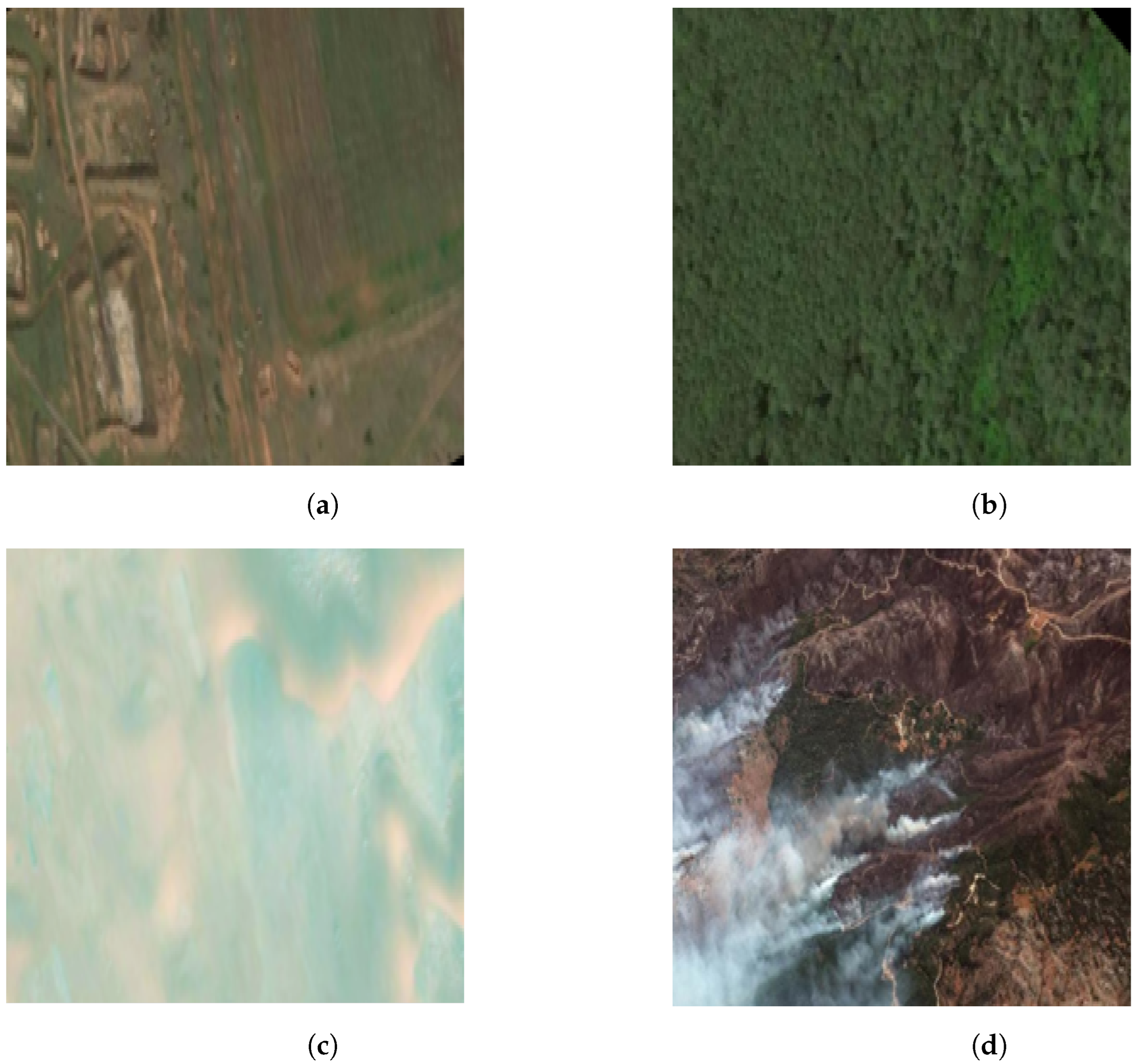
As mentioned above, various methods have been used for anomaly detection. Here, we consider the Vision Transformer with Masked Autoencoder as a model for anomaly detection and the Grad-CAM method that can be used to create saliency areas.

2.1. Dataset

The training dataset for the base (pre-trained) AE model was the ImageNet-1K image dataset. This dataset consists of 1,128,167 training images, 50,000 validation images, and 100,000 test images divided into 1000 labeled classes [40]. The Vision Transformer (ViT) model pre-trained using the MAE method was obtained from the HuggingFace model hub.
To fine-tune the model parameters and for validation, a custom dataset was built. We acquired 317 satellite images using the Mapbox API v3.1.0 [41]. The images were later divided into two parts, one representing the normal sample dataset (197 samples) and the other representing the anomaly dataset (120 samples). Regarding the train–test split, the dataset was divided in such a way that the test set consisted of 120 samples from each class. Only the remaining normal samples were used for training.
The data was then preprocessed using TensorFlow’s 2.17.0 image preprocessing layers, and a data augmentation step was performed for the fine-tuning training phase. With random horizontal and vertical rotation flips, random rotation and auto-contrast applied, the training dataset was artificially enlarged to balance the train–test ratio. All the operations were performed using the torchvision.transforms module. RandomRotation with an angle in the range of (0, 45) degrees was applied to each image. RandomAutocontrast was applied with default probability p = 0.5. RandomHorizontalFlip was applied with probability p = 0.2. The same probability was reused in RandomVerticalFlip. Two samples from the dataset are presented in Figure 2, divided into anomaly and normal classes.
To divide the dataset into normal and abnormal classes, the following rules were applied. Pictures with homogeneous environments, included forests, deserts, and full maritime areas. Pictures depicting planes, starting lanes, ships deployed on full seas, and changes or gaps within crops were identified as anomalies. Examples of classification are shown in Figure 2. However, the division rules are subjective. They reflect the specificity of real-life applications where anomalies occur sparsely, meaning there is also a requirement for an unbalanced dataset.

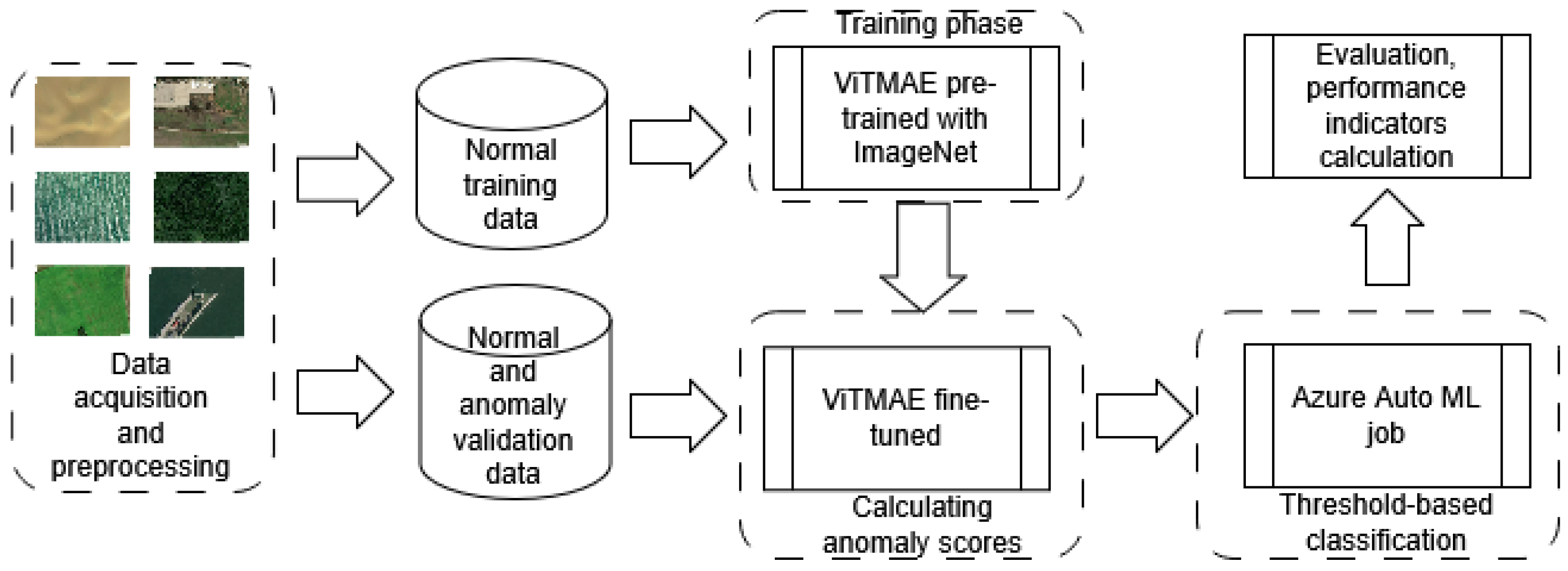
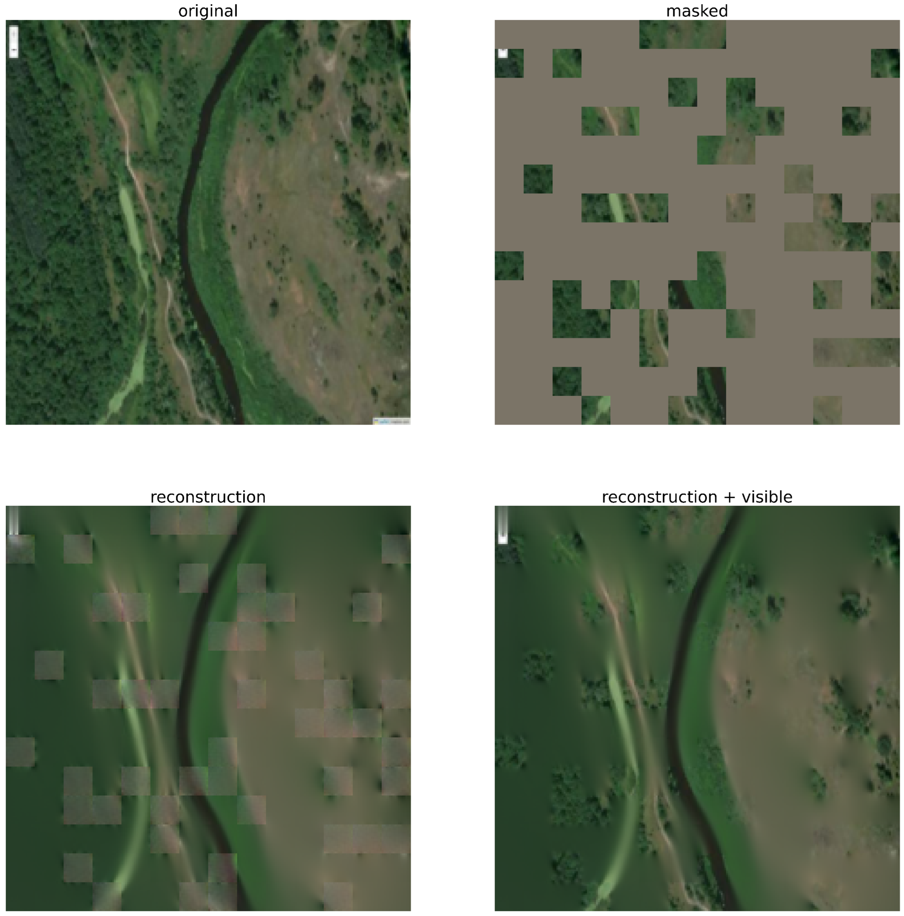
2.2. Proposed Approach

The visual masked autoencoder used for the purpose of this paper was the model used in [42]. Here, the autoencoder is organized in an asymmetric design that allows the model to operate only on partial information during handling input images while the remaining tokens are masked. The patches that were chosen to be masked were selected according to a uniform distribution to ensure equal and non-deterministic masking. Other issues that were taken into account were the requirement to disable the algorithm from creating extrapolations of neighboring patches and to exclude center bias, which is primarily visible when patches around the image center are masked. It should be mentioned that the original encoder–decoder architecture was published in [43] and was reused in [42]. In this model, each single image is divided into equal patches that pass through parallel linear projection modules. Next, a learnable embedding is created in the sequence of embedded patches to model image representation. Position embeddings are added to the patch embeddings to retain positional information. The Transformer encoder [1] consists of alternating layers of multi-headed self-attention and multi-layer perceptron blocks. Layer normalization is applied before each block. The model used in our research, the ViTMAE Large variant, uses 24 layers combined with 16 self-attention heads. The Masked Autoencoder reconstructs the input by predicting the input pixel values for each patch that was previously masked. The last layer of the decoder is a linear projection with the number of output channels equal to the number of pixel values in a patch. The decoder output is then reshaped to form a reconstructed image. This process is the basis for loss function calculations. The loss for the model is calculated as Mean Squared Error between the reconstructed and original images in the pixel space. The non-masked pixels are not considered. After the reconstruction error is calculated for each image in the validation dataset, the results are stored for a later training phase. With the acquired data, a second classification model is added to the pipeline to classify samples based on the reconstruction error rate. Using Microsoft Azure’s Automated Machine Learning (SDK v2) software, a threshold-based classification task is performed. The task selects a threshold that results in the best performance indicators. Then, the threshold is applied in the final model.

2.3. Grad-CAM Method

The Grad-CAM method [44] can be used to determine saliency areas. This method is useful for assessing and understanding the decision-making of neural networks. The Grad-CAM method utilizes the gradient information flowing into the final convolutional layer to assign weight values to each neuron for a particular decision, and it is a generalization of the Class Activation Mapping (CAM) method. It highlights important class-specific regions of the input images during one forward propagation and partial back propagation for each image.
As depicted in [44], to obtain a L G r a d C A M C saliency map for class c, we first calculate the gradient of the result of the last layer of the network before softmax y c with respect to the feature map activation A k of the convolutional layer. After obtaining the multidimensional gradients, the global average pooling technique is used to show the importance of each feature map for specific classes (over two dimensions: width i and height j). Therefore, to calculate the neurone weight α k c , which represents a partial linearization of the deep network downstream from A, the following equation is used:
α k c = 1 Z i j y c A i j k .
The weights α k c are multiplied by the corresponding feature maps A k , we sum up the components of the final saliency map, and the weighted combination of forward activation maps followed by the ReLU is performed as follows:
L G r a d C A M C = R e L U ( k α k c A k ) .

3. Results and Discussion

The training was performed using the PyTorch programming library and the Python v.3 environment. As an optimizer, Stochastic Gradient Descent was used. The training was performed for 10 epochs with a randomly selected batch of training images for each epoch.
Hyperparameters for the output model were tuned using the Grid Search cross-validation method. All of the results presented in this section were obtained for the best set of hyperparameters (learning rate, batch size, number of learning epochs). The same approach was applied to PyTorch’s v2.5.0 ViTMAE model. However, the Grid Search method does not guarantee that the set of output parameters and hyperparameters is optimal. It provides a method for exploring the search space that yields satisfactory results.

3.1. Trained Architecture

After training the model with the parameters described in the previous chapter, it was tested on the provided dataset. The visualization of the autoencoder working part is shown in Figure 3.
The figure contains four pictures. The first of them presents the original image, while the second presents the masked one. The next two are outputs of the processing pipeline. The figure described as ‘reconstruction’ contains the image reconstructed by the autoencoder. The last image presented shows a reconstructed image with patches that were visible to the autoencoder, i.e., copied from the original image. The analysis allows us to draw the following conclusion: the trained model is capable of reconstructing general shapes and homogeneous images, with higher reconstruction error, when there are more details in the image or there is a heterogeneous change within the regular environment. After the model was evaluated, a thorough analysis was performed to verify the interpretability of the model in terms of correctly and incorrectly classified samples from the dataset. The results of the analysis are shown in Figure 4.
Looking at Figure 4, we can see the image samples that were the subject of the final classification. The images are transformed according to random horizontal and vertical rotation flip, random rotation, and auto-contrast methods. Figure 4b shows an example of a correctly classified normal sample, while Figure 4a depicts an anomaly. We can state that the system works correctly for homogenous images without man-made objects, while Figure 4a shows some trenches of military training dug out. On the other hand, Figure 4c presents undetected signs of wildfires in the environment. Also, as shown in Figure 4d, some terrains with regular shape may be taken as anomalies by the proposed system. In terms of the reconstruction error (indicated by the value of the loss function), it can be visualized for further analysis with the histograms presented in Figure 5.
The histograms show that the loss function values tend to be concentrated for normal samples, whereas they tend to be more distributed for anomalous images. In addition, the overall reconstruction error is lower for normal images, which confirms the hypothesis stated that known images are reconstructed in a better way than novel, unfamiliar images.
To address the problem of assessing the confidence level, we propose a formula that derives from the calculated anomaly score. The indicator is proportional to the absolute value of the difference between the anomaly score for a given sample and the threshold. In the case of the reconstruction problem, the threshold value should be set at 0.5, meaning the closer the anomaly score is to 0, the more certain model’s output is when predicting normal samples. On the other hand, the closer the value is to 1, the higher the error that the estimator reconstructss the image with, i.e., the probability of spotting an anomaly is higher. To scale values and obtain the final range from 0 to 1, the obtained value should be multiplied by 2. The final formula for the confidence level for the task can be described with Formula (3), as follows:
c o n f i d e n c e _ l e v e l = 2 · | ( a n o m a l y _ s c o r e 0.5 ) |
Several performance indicators, i.e., accuracy, precision, recall, and F1 score, have been calculated according to Formulas (4a)–(4d). Accuracy is a quality factor that refers to the percentage of correctly classified images. Precision is the ratio of true positives to all images classified as true and false positives. The recall factor (or sensitivity) is a proportion of actual positives that are correctly classified. In turn, the F1 score is interpreted as a harmonic mean of precision and recall scores.
a c c u r a c y = T P + T N T P + T N + F P + F N
p r e c i s i o n = T P T P + F P
r e c a l l = T P T P + F N
F 1 s c o r e = 2 · T P 2 · T P + F P + F N
The following rules were applied when calculating performance indicators:
  • TP (True Positive) = a sample classified as an anomaly that is truly an anomaly;
  • FP (False Positive) = a sample classified as an anomaly, but in fact is from the normal class;
  • FN (False Negative) = a sample classified as normal, but in fact is an anomaly;
  • TN (True Negative) = a sample classified as normal that truly belongs to the normal class.
The performance indicators for the best binary classifier are presented in Table 1.
The confusion matrix for the final model is presented in Table 2.

3.2. Results Obtained by the Grad-CAM Method

Terms such as explainability and eXplainable AI (XAI) are current emerging approaches to improving model interpretability and the rules that lie behind neural network models. To apply the Grad-CAM method, an adaptation step was required to transfer knowledge between the autoencoder model and the standard multiclass classifier architecture for which the Grad-CAM method was proposed. For this task, after training the ViTMAE model on our custom dataset and updating its weights, we divided the autoencoder into two halves: the encoder and decoder. The encoder part was then used as the hidden layers of the standard classifier with an additional sequential layer for multiclass classification, in the same manner as the classifier proposed in [36] was created. The results of running the Grad-CAM algorithm for samples from a custom dataset are shown in Figure 6.
After analysing the results obtained, it is clear that the model cannot properly identify the features of each image and locate the most crucial objects that could potentially lead to anomaly detection. Taking into account the bottom right example in Figure 6, the model misleadingly chose the object and natural habitat around the potentially suspicious building as the center of interest. Furthermore, looking at the bottom left example, we see that the model did not spot the entire airstrip with aircraft visible, taking into account the homogenous area around it as a base for classification. In contrast, the analysis of the Grad-CAM results showed that the model in some cases was capable of making correct decisions, which is demonstrated by the top right example in Figure 6. In general, the model proposed in this paper was capable of spotting only a subset of the anomalies present in the dataset, which implies the need to improve the model’s capabilities and performance.

3.3. Additional Experiments

Furthermore, we decided to evaluate the model on a smaller and more homogeneous dataset. In this case, the uniformity of the dataset meant choosing a subset of images that represented terrains with similar features. Thus, from the original dataset, a subset of 100 images was set. This new dataset consisted of images of forests and fields, with 10% of them described as abnormal. Examples from the newly constructed dataset are presented in Figure 7 and Figure 8.
The approach presented in Section 3.1 was applied to the new dataset. The model training process output is presented in Figure 9. The main goal of the experiment was to observe the model’s behavior for less diverse datasets. The results of the experiment show that the model’s accuracy and precision tend to be significantly better compared to the original experiment. The average accuracy obtained was 81% and the recall was 80%. All averaged performance indicators are summarized in Table 3.
However, the obtained results for precision seem to be insufficient, and we assume that the recall is valued higher in the case of anomaly detection for aerial imagery. In this case, we expect the classifier to have lower precision. The results can also be seen from the confusion matrix (Table 4).

3.4. Grad-CAM Results Obtained for Revisited Dataset

For the purpose of evaluating the model trained on the modified dataset, the approach described in Section 3.2 was replicated. The results of the Grad-CAM analysis for the sample images of the constructed dataset are presented in Figure 10.
The figure presents the model’s output activation heatmaps for both the anomalous (bottom right corner) and normal samples. By looking at the original counterparts, we can see that the model correctly detects novelty changes in the environment. However, looking at the normal representatives, it can be seen that the output of regular and consistent images appears to be indeterministic, as the model attempts to create an internal representation of regular data with irregular shapes.

4. Conclusions

The results presented in this paper can be viewed as a demonstration of a general approach to the anomaly detection task. Model evaluation shows that, in general, this approach may be successfully applied to different models that are assembled into an encoder–decoder architecture. However, it is also crucial to note that the anomaly detection accuracy results are considerably lower for the custom dataset. It is also worth mentioning that the results may be influenced by the low resolution and the level of detail present in each image from the custom dataset. This paper addresses the first use of the fine-tuned Masked Vision Transformer Autoencoder for a custom-built satellite image dataset. The classifier was trained in a self-supervised manner. The experiment described in Section 3.3 could be treated as a proof of concept for the method to be used in different datasets and in different but more uniform environments. Inferring from the experiment, it can be stated that the model designed for the experiment was not capable of discriminating between different and diverse environment samples and one should limit the area of interest to a single type of landscape or scenery. However, the model was not sufficiently effective to be applied to the general task of anomaly detection for all possible types of satellite images, and it was shown that fine-tuned models were capable of detecting novelties for a custom dataset. Additionally, with an established image resolution, the problem can be transferred to aerial images and applied in various related fields.

Author Contributions

Conceptualization, J.G. and J.K.; methodology, J.G. and J.K.; software, J.G.; validation, J.G.; formal analysis, J.G.; investigation, J.G. and J.K.; resources, J.G.; data curation, J.G.; writing—original draft preparation, J.G.; writing—review and editing, J.G. and J.K.; visualization, J.G.; supervision, J.K.; project administration, J.G.; funding acquisition, J.K. All authors have read and agreed to the published version of the manuscript.

Funding

This research was supported by a research subsidy from AGH University of Krakow 16.16.120.773.

Institutional Review Board Statement

Not applicable.

Informed Consent Statement

Not applicable.

Data Availability Statement

The dataset used is the ImageNet-1K dataset (openly available on https://www.image-net.org/download.php (accessed on 12 June 2024)).

Conflicts of Interest

The authors declare no conflicts of interest.

Abbreviations

The following abbreviations are used in this manuscript:
AEAutoencoder
Grad-CAMGradient-based Class Activation Mapping
MAEMasked Autoencoder
ViTVision Transformer
ViTMAEVision Transformer with Masked Autoencoder

References

  1. Vaswani, A.; Shazeer, N.; Parmar, N.; Uszkoreit, J.; Jones, L.; Gomez, A.N.; Kaiser, Ł.; Polosukhin, I. Attention is all you need. In Proceedings of the Neural Information Processing Systems, Long Beach, CA, USA, 4–9 December2017; Volume 2017.
  2. ChatGPT. 2023. Available online: https://openai.com/chatgpt (accessed on 17 October 2014).
  3. DALL-E. 2023. Available online: https://openai.com/dall-e-3 (accessed on 17 October 2014).
  4. What Is a Transformer Model? 2023. Available online: https://blogs.nvidia.com/blog/2022/03/25/what-is-a-transformer-model/ (accessed on 17 October 2014).
  5. Yang, J.; Xu, R.; Qi, Z.; Shi, Y. Visual anomaly detection for images: A survey. arXiv 2021, arXiv:2109.13157. [Google Scholar]
  6. Patcha, A.; Park, J.M. An overview of anomaly detection techniques: Existing solutions and latest technological trends. Comput. Netw. 2007, 51, 3448–3470. [Google Scholar] [CrossRef]
  7. Barnett, V.; Lewis, T. Outliers in Statistical Data; Wiley: New York, NY, USA, 1994; Volume 3. [Google Scholar]
  8. Elmrabit, N.; Zhou, F.; Li, F.; Zhou, H. Evaluation of machine learning algorithms for anomaly detection. In Proceedings of the IEEE Cyber Security, Dublin, Ireland, 15–19 June 2020; pp. 1–8. [Google Scholar]
  9. Spillner, A.; Linz, T. Software Testing Foundations: A Study Guide for the Certified Tester Exam-Foundation Level-ISTQB® Compliant; Rocky Nook: San Rafael, CA, USA, 2021. [Google Scholar]
  10. Eskin, E. Anomaly Detection over Noisy Data using Learned Probability Distributions. In Proceedings of the International Conference on Machine Learning (ICML ’00), San Francisco, CA, USA, 29 June–2 July 2000; pp. 255–262. [Google Scholar]
  11. Klerx, T.; Anderka, M.; Büning, H.K.; Priesterjahn, S. Model-based anomaly detection for discrete event systems. In Proceedings of the IEEE International Conference on Tools for Artificial Intelligence (ICTAI), Limassol, Cyprus, 10–12 November 2014; pp. 665–672. [Google Scholar]
  12. Ruff, L.; Vandermeulen, R.A.; Gornitz, N.; Binder, A.; Muller, E.; Kloft, M. Deep support vector data description for unsupervised and semi-supervised anomaly detection. In Proceedings of the International Conference on Machine Learning (ICML) Workshop on Uncertainty and Robustness in Deep Learning, Long Beach, CA, USA, 14 June 2019; pp. 9–15. [Google Scholar]
  13. Lesouple, J.; Baudoin, C.; Spigai, M.; Tourneret, J.Y. Generalized isolation forest for anomaly detection. Pattern Recognit. Lett. 2021, 149, 109–119. [Google Scholar] [CrossRef]
  14. Wang, Y.; Wong, J.; Miner, A. Anomaly intrusion detection using one class SVM. In Proceedings of the 5th IEEE Systems, Man, and Cybernetics (SMC) Information Assurance Workshop, New York, NY, USA, 10–11 June 2004; pp. 358–364. [Google Scholar]
  15. Sheridan, K.; Puranik, T.G.; Mangortey, E.; Pinon-Fischer, O.J.; Kirby, M.; Mavris, D.N. An application of dbscan clustering for flight anomaly detection during the approach phase. In Proceedings of the American Institute of Aeronautics and Astronautics Scitech Forum, Orlando, FL, USA, 6–10 January 2020; p. 1851. [Google Scholar]
  16. Wibisono, S.; Anwar, M.T.; Supriyanto, A.; Amin, I.H.A. Multivariate weather anomaly detection using DBSCAN clustering algorithm. In Journal of Physics: Conference Series (JPCS); IOP Publishing: Bristol, UK, 2021; Volume 1869, p. 012077. [Google Scholar]
  17. Liu, F.T.; Ting, K.M.; Zhou, Z.H. Isolation forest. In Proceedings of the IEEE International Conference on Data Mining (ICDM), Pisa, Italy, 15–19 December 2008; pp. 413–422. [Google Scholar]
  18. Malhotra, P.; Vig, L.; Shroff, G.; Agarwal, P. Long Short Term Memory Networks for Anomaly Detection in Time Series. In Proceedings of the European Symposium on Artificial Neural Networks (ESANN), Bruges, Belgium, 22–24 April 2015; Volume 2015, p. 89. [Google Scholar]
  19. An, J.; Cho, S. Variational autoencoder based anomaly detection using reconstruction probability. Spec. Lect. IE 2015, 2, 1–18. [Google Scholar]
  20. Xia, X.; Pan, X.; Li, N.; He, X.; Ma, L.; Zhang, X.; Ding, N. GAN-based anomaly detection: A review. Neurocomputing 2022, 493, 497–535. [Google Scholar] [CrossRef]
  21. Vareldzhan, G.; Yurkov, K.; Ushenin, K. Anomaly detection in image datasets using convolutional neural networks, center loss, and mahalanobis distance. In Proceedings of the IEEE Ural-Siberian Conference on Biomedical Engineering, Radioelectronics and Information Technology (USBEREIT), Yekaterinburg, Russia, 13–14 May 2021; pp. 387–390. [Google Scholar]
  22. Sarafijanovic-Djukic, N.; Davis, J. Fast distance-based anomaly detection in images using an inception-like autoencoder. In Proceedings of the Discovery Science (DS2019), Split, Coratia, 28–30 October 2019; Springer: Cham, Switzerland, 2019; pp. 493–508. [Google Scholar]
  23. Staar, B.; Lütjen, M.; Freitag, M. Anomaly detection with convolutional neural networks for industrial surface inspection. CIRP 2019, 79, 484–489. [Google Scholar] [CrossRef]
  24. Togo, R.; Watanabe, H.; Ogawa, T.; Haseyama, M. Deep convolutional neural network-based anomaly detection for organ classification in gastric X-ray examination. Comput. Biol. Med. 2020, 123, 103903. [Google Scholar] [CrossRef] [PubMed]
  25. Siddalingappa, R.; Kanagaraj, S. Anomaly detection on medical images using autoencoder and convolutional neural network. Int. J. Adv. Comput. Sci. Appl. 2021, 12, 148–156. [Google Scholar] [CrossRef]
  26. Zhou, Z.; Sodha, V.; Siddiquee, M.M.R.; Feng, R.; Tajbakhsh, N.; Gotway, M.B.; Liang, J. Models genesis: Generic autodidactic models for 3d medical image analysis. In Proceedings of the Medical Image Computing and Computer Assisted Interventions (MICCAI), Shenzhen, China, 13–17 October 2019; Springer: Berlin/Heidelberg, Germany, 2019; pp. 384–393. [Google Scholar]
  27. Khan, A.S.; Ahmad, Z.; Abdullah, J.; Ahmad, F. A spectrogram image-based network anomaly detection system using deep convolutional neural network. IEEE Access 2021, 9, 87079–87093. [Google Scholar] [CrossRef]
  28. Goh, J.; Adepu, S.; Tan, M.; Lee, Z.S. Anomaly detection in cyber physical systems using recurrent neural networks. In Proceedings of the IEEE HASE, Singapore, 12–14 January 2017; pp. 140–145. [Google Scholar]
  29. Huang, H.; Wang, P.; Pei, J.; Wang, J.; Alexanian, S.; Niyato, D. Deep Learning Advancements in Anomaly Detection: A Comprehensive Survey. arXiv 2025, arXiv:2503.13195. [Google Scholar]
  30. Zhang, X.; Li, N.; Li, J.; Dai, T.; Jiang, Y.; Xia, S.T. Unsupervised Surface Anomaly Detection with Diffusion Probabilistic Model. In Proceedings of the 2023 IEEE/CVF International Conference on Computer Vision (ICCV), Paris, France, 1–6 October 2023; pp. 6759–6768. [Google Scholar] [CrossRef]
  31. Li, D.; Chen, D.; Goh, J.; Ng, S.K. Anomaly detection with generative adversarial networks for multivariate time series. arXiv 2018, arXiv:1809.04758. [Google Scholar]
  32. Schlegl, T.; Seeböck, P.; Waldstein, S.M.; Schmidt-Erfurth, U.; Langs, G. Unsupervised anomaly detection with generative adversarial networks to guide marker discovery. In Proceedings of the Information Processing in Medical Imaging (IPMI), Boone, NC, USA, 25–30 June 2017; Springer: Berlin/Heidelberg, Germany, 2017; pp. 146–157. [Google Scholar]
  33. Zhang, J.; Wang, C.; Li, X.; Tian, G.; Xue, Z.; Liu, Y.; Pang, G.; Tao, D. Learning Feature Inversion for Multi-class Anomaly Detection under General-purpose COCO-AD Benchmark. arXiv 2024, arXiv:2404.10760. [Google Scholar]
  34. Seeböck, P.; Waldstein, S.; Klimscha, S.; Gerendas, B.S.; Donner, R.; Schlegl, T.; Schmidt-Erfurth, U.; Langs, G. Identifying and categorizing anomalies in retinal imaging data. arXiv 2016, arXiv:1612.00686. [Google Scholar]
  35. Richter, C.; Roy, N. Safe visual navigation via deep learning and novelty detection. In Robotics: Science and Systems XIII; Massachusetts Institute of Technology: Cambridge, MA, USA, 2017. [Google Scholar]
  36. Xia, Y.; Cao, X.; Wen, F.; Hua, G.; Sun, J. Learning discriminative reconstructions for unsupervised outlier removal. In Proceedings of the International Conference on Computer Vision (ICCV), Santiago, Chile, 7–13 December 2015; pp. 1511–1519. [Google Scholar]
  37. ViTMAE Document Page. 2023. Available online: https://huggingface.co/docs/transformers/main/model_doc/vit_mae (accessed on 10 December 2024).
  38. Castillo-Villamor, L.; Hardy, A.; Bunting, P.; Llanos-Peralta, W.; Zamora, M.; Rodriguez, Y.; Gomez-Latorre, D.A. The Earth Observation-based Anomaly Detection (EOAD) system: A simple, scalable approach to mapping in-field and farm-scale anomalies using widely available satellite imagery. Int. J. Appl. Earth Obs. Geoinf. 2021, 104, 102535. [Google Scholar] [CrossRef]
  39. Wang, H.; Yu, W.; You, J.; Ma, R.; Wang, W.; Li, B. A unified framework for anomaly detection of satellite images based on well-designed features and an artificial neural network. Remote Sens. 2021, 13, 1506. [Google Scholar] [CrossRef]
  40. Russakovsky, O.; Deng, J.; Su, H.; Krause, J.; Satheesh, S.; Ma, S.; Huang, Z.; Karpathy, A.; Khosla, A.; Bernstein, M.; et al. ImageNet Large Scale Visual Recognition Challenge. Int. J. Comput. Vis. 2015, 115, 211–252. [Google Scholar] [CrossRef]
  41. Mapbox. Available online: https://www.mapbox.com/ (accessed on 5 August 2024).
  42. He, K.; Chen, X.; Xie, S.; Li, Y.; Dollár, P.; Girshick, R.B. Masked Autoencoders Are Scalable Vision Learners. arXiv 2021, arXiv:2111.06377. [Google Scholar]
  43. Dosovitskiy, A.; Beyer, L.; Kolesnikov, A.; Weissenborn, D.; Zhai, X.; Unterthiner, T.; Dehghani, M.; Minderer, M.; Heigold, G.; Gelly, S.; et al. An image is worth 16 × 16 words: Transformers for image recognition at scale. In Proceedings of the International Conference on Learning Representations (ICLR), Vienna, Austria, 4 May 2021. [Google Scholar]
  44. Selvaraju, R.R.; Cogswell, M.; Das, A.; Vedantam, R.; Parikh, D.; Batra, D. Grad-CAM: Visual Explanations from Deep Networks via Gradient-Based Localization. Int. J. Comput. Vis. 2020, 128, 336–359. [Google Scholar] [CrossRef]
Figure 1. Proposed framework, consisting of training and validation pipelines.
Applsci 15 06286 g001
Figure 2. Comparison of normal vs. anomalous samples. (a) Sample of normal image. (b) Sample of anomalous image.
Applsci 15 06286 g002
Figure 3. Image reconstruction results for a single image with possible combinations.
Applsci 15 06286 g003
Figure 4. Examples of obtained classification output for each confusion matrix class. (a) Example of correctly classified anomaly sample. (b) Example of correctly classified normal sample. (c) Example of misclassified normal sample. (d) Example of misclassified anomaly sample.
Applsci 15 06286 g004
Figure 5. Loss function histograms for both classes. (a) Histogram of loss function value for the normal dataset. (b) Histogram of loss function value for the anomalous dataset.
Applsci 15 06286 g005
Figure 6. Sample results for running Grad-CAM method compared with original images from custom dataset.
Applsci 15 06286 g006
Figure 7. Samples of anomalies identified in the second experiment. (a) Anomaly example of military trenches. (b) Anomaly example of military base starting lane.
Applsci 15 06286 g007
Figure 8. Samples of normal class from homogenous dataset. (a) Normal example of forest area. (b) Normal example of forest area. (c) Normal example of forest area. (d) Normal example of crop area.
Applsci 15 06286 g008
Figure 9. Learning process for proposed model.
Applsci 15 06286 g009
Figure 10. Results of applying Grad-CAM method for samples taken from additional dataset (on the right), together with original images (on the left) for comparison.
Applsci 15 06286 g010
Table 1. Performance indicators for the evaluated system.
AccuracyPrecisionRecallF1 Score
0.490.490.670.57
Table 2. Confusion matrix for the evaluated system.
Predicted AnomalyPredicted Normal
True anomaly763
True normal2960
Table 3. The performance indicators for the evaluated system.
AccuracyPrecisionRecallF1 Score
0.810.320.80.46
Table 4. Confusion matrix for the evaluated system.
Predicted AnomalyPredicted Normal
True anomaly82
True normal1773
Disclaimer/Publisher’s Note: The statements, opinions and data contained in all publications are solely those of the individual author(s) and contributor(s) and not of MDPI and/or the editor(s). MDPI and/or the editor(s) disclaim responsibility for any injury to people or property resulting from any ideas, methods, instructions or products referred to in the content.

