Remote Sensing-Based Multilayer Perceptron Model for Grassland Above-Ground Biomass Estimation

Abstract

Above-ground biomass (AGB) is a core indicator for evaluating grassland ecosystem health and carbon storage. Traditional ground-based AGB measurements are labor-intensive and ill suited for large-scale monitoring. This study addresses this gap by developing a Multilayer Perceptron (MLP) model integrating Landsat 9 OLI/TIRS imagery acquired on 15 August 2024, with ground data from 78 sampling points (62 training, 16 testing). Incorporating fourteen multi-source features (seven vegetation indices, e.g., Modified Vegetation Index (MVI) and Green Chlorophyll Index (CIg); four meteorological variables; three soil properties), all data were standardized via z-score normalization before training. The MLP model, optimized via six-fold cross-validation, achieved an R² of 0.765 and RMSE of 38.066 g/m², outperforming XGBoost (R² = 0.723, RMSE = 41.354 g/m²) with a statistically significant 5.8% accuracy improvement (p < 0.05). Spatial analysis revealed a north-to-south AGB gradient, strongly correlated with precipitation gradients (250–350 mm/year) and soil organic carbon (R = 0.428). These findings provide a robust framework for climate-adaptive grassland management and carbon assessment in semi-arid regions.

1. Introduction

Grasslands are one of the most widely distributed vegetation types globally, covering approximately 25% of the Earth’s surface and storing approximately 34% of global soil carbon [1], with Inner Mongolia’s grasslands alone accounting for 1.79 PgC [2]. Tang et al.’s national-scale machine learning model identified precipitation as a critical predictor for forest aboveground biomass (AGB) across China, reinforcing its role in shaping carbon storage potential in diverse ecosystems [3]. They play an extremely important role in the global ecosystem. Grasslands not only act as crucial carbon and nitrogen reservoirs, effectively mitigating the adverse effects of global climate change, but also play a key role in water conservation, soil protection, and biodiversity maintenance [4]. Above-ground biomass (AGB), a key indicator of grassland health, directly influences carbon sequestration capacity. For instance, Wu et al. found that AGB in Xilinhot ranges from 120 g/m² (desert steppe) to 350 g/m² (meadow steppe), with soil organic carbon (SOC) contributing 32% to this spatial variation—a relationship critical for regional carbon accounting [5]. Therefore, accurately estimating AGB over large areas is of great practical significance for scientifically assessing the ecological health of grasslands, developing reasonable grassland resource management strategies, and maintaining regional ecological security.

Traditional ground-based harvesting methods, while precise, are labor-intensive and limited to small scales. For example, Zhou et al.’s comprehensive review revealed that traditional field measurement methods for grassland AGB require destructive sampling of numerous quadrats (typically 30–50 plots per hectare), making large-scale monitoring labor-intensive and ecologically disruptive [6]. Although this method provides high precision, it also has clear limitations [6]. On one hand, the ground harvesting method is complex, time-consuming, and costly, making it unsuitable for large-scale, long-term dynamic monitoring. On the other hand, because it is limited to a small sample area, it cannot meet the demand for biomass estimation at large spatial scales. As global environmental changes intensify, there is an increasing need for efficient and accurate large-scale dynamic monitoring of grassland biomass.

In contrast, remote sensing technology, with its wide spatial coverage, high timeliness, and relatively low cost, has become an ideal tool for large-scale grassland biomass monitoring [7]. By obtaining wide-area spectral information, remote sensing imagery can provide data related to grassland vegetation cover, canopy structure, and growth conditions, which can be further used to extract vegetation indices and other variables closely related to biomass [8]. In recent years, with the enrichment of remote sensing data sources and the improvement of resolution, researchers have gradually explored statistical models based on the relationship between spectral reflectance, vegetation indices, and biomass. These methods can not only achieve large-scale grassland biomass estimation but also partially overcome the limitations of traditional ground-based measurement methods [9].

Moreover, some researchers have combined remote sensing data with crop growth models to simulate grassland biomass [10]. However, crop growth models rely heavily on numerous environmental factors (such as water and soil nutrients) and ecological theories for biomass estimation, making them dependent on large amounts of data. This reliance makes it difficult to meet the practical demand for rapid and large-scale estimation of grassland biomass [11]. Against this backdrop, remote sensing-based biomass inversion models using machine learning algorithms have gradually emerged. Machine learning models, due to their powerful data processing and nonlinear fitting capabilities, can establish mapping relationships between grassland biomass and variables such as vegetation indices, terrain, and soil, by learning from a large amount of historical data. These models demonstrate strong robustness, and even with limited data, they can still provide reliable biomass estimation results, making them effective tools for remote sensing-based grassland biomass inversion [12].

However, most existing machine learning models for AGB estimation still rely on single vegetation indices (e.g., NDVI) or neglect the coupled effects of terrain, climate, and soil factors [13]. For example, models using only spectral data have shown poor performance in mountainous regions with high spatial heterogeneity, where topographic shading and soil nutrient gradients strongly influence biomass distribution. Although auxiliary variables like meteorological data have been introduced, the nonlinear interactions between multi-source features are often oversimplified in traditional algorithms, limiting estimation accuracy in complex ecosystems [14,15]. This study addresses this gap by leveraging MLP’s deep learning architecture to capture hierarchical relationships among vegetation, environment, and biomass.

In machine learning algorithms, Multilayer Perceptron (MLP), as a typical deep learning model, has been widely applied to complex environmental variable estimation and classification tasks in recent years due to its multilayer network structure and powerful nonlinear fitting capability. MLP can effectively capture the combined effects of vegetation indices, meteorological data, terrain, and soil on grassland biomass, making it highly suitable for biomass inversion tasks [16].

Against this background, this study aims to achieve the following: ① develop an MLP model integrating vegetation indices, meteorological data, topographic features, and soil properties to achieve high-precision AGB estimation in heterogeneous grasslands; ② quantitatively compare the performance of MLP with five traditional machine learning models (RF, XGBoost, SVR, MLR, GBDT) in capturing nonlinear feature interactions; ③ analyze the spatial distribution patterns of AGB in Xiwuzhumuqin Banner and identify key environmental drivers (e.g., precipitation, soil organic carbon) using correlation and regression analysis; ④ provide a scalable remote sensing framework for large-scale grassland monitoring, supporting sustainable grazing management and carbon sequestration assessments.

This study focuses on the Xilinhot region in Inner Mongolia, utilizing Landsat 9 remote sensing data combined with ground-truth measurements to construct a Multilayer Perceptron (MLP) model based on vegetation indices, meteorological data, terrain data, and soil data for precise inversion of grassland above-ground biomass. Additionally, the performance of the MLP model will be compared with traditional machine learning models such as Random Forest (RF), Extreme Gradient Boosting (XGBoost), and Support Vector Regression (SVR) to explore the applicability and accuracy of different models in grassland biomass estimation. The results of this study will provide scientific support for dynamic monitoring and resource management of grassland ecosystems, as well as data support for the sustainable use and ecological protection strategies of grassland resources.

2. Overview of the Study Area

As it can be seen in Figure 1, Xiwuzhumuqin Banner (abbreviated as Xiwuzhumuqin or Xiwuzhumuqin Qi) is located in the central part of Inner Mongolia, in the eastern part of Xilingol League. The geographical coordinates range from 43°52′ N to 45°23′ N and 116°21′ E to 119°23′ E, covering a total area of 22,435 km². It borders Dongwuzhumuqin Banner to the north, Arukorqin Banner to the east, Balin Left Banner, Balin Right Banner, Linxi County, and Keshiketeng Banner to the south, and is adjacent to Xilinhot City to the west. The terrain of the region slopes from the southeast to the northwest, with an elevation range between 835 m and 1957 m, and an average elevation of over 1000 m. The main landforms include mountains, low mountain hills, and undulating plateaus. Mountains account for 24.9%, low mountain hills cover 27.7%, and plateaus make up 40.5% of the region’s total area [17].

Xiwuzhumuqin Banner was selected as the study area for its ecological and methodological significance. Ecologically, it is dominated by typical steppe ecosystems, which serve as a critical carbon sink and grazing resource in Inner Mongolia’s grassland belt. The region’s diverse microclimates, ranging from arid northwest (250 mm annual precipitation) to semi-humid southeast (350 mm), and topographic gradients (elevation 835–1957 m) create heterogeneous conditions ideal for testing multi-source data models. Methodologically, its large spatial extent (22,435 km²) and relatively undisturbed grassland landscapes provide a representative dataset for scaling remote sensing applications to similar semi-arid regions globally.

In terms of climate, precipitation is uneven and varies significantly from year to year. The annual precipitation in the northwest is about 250 mm, while in the southeast it exceeds 350 mm, with the majority falling between July and August. The region has diverse soil types, with the predominant ones being chestnut calcareous soil (62.42%) and black calcareous soil (13.19%). The grassland types in this area mainly include meadow steppe, typical steppe, and wetland steppe. Major plant species include Stipa grandis, Leymus chinensis, Cleistogenes squarrosa, Artemisia frigida, and Agropyron cristatum [18].

3. Data Acquisition and Preprocessing

To achieve accurate inversion of grassland above-ground biomass in Xiwuzhumuqin Banner, this study integrates multiple types of data, including spectral reflectance data, terrain data, soil nutrient data, ground-truth biomass data, and meteorological data, based on the geographical, climatic, and ecological characteristics of the study area. These data are sourced from various platforms with different temporal and spatial resolutions, and through comprehensive processing, they can reflect the spatial distribution characteristics of grassland biomass in the study area.

3.1. Remote Sensing Data Acquisition and Preprocessing

Remote sensing data is the fundamental data source for constructing the grassland above-ground biomass inversion model in this study. To obtain the spectral reflectance characteristics of the grassland vegetation in the study area, Landsat 9 remote sensing imagery was selected as the primary data source. Landsat 9 imagery has a spatial resolution of 30 m, which can clearly capture vegetation cover and canopy reflectance characteristics, meeting the needs for precise biomass estimation. In this study, Landsat 9 Level 2 data were downloaded from the US Geological Survey (USGS) Earth Explorer platform (https://earthexplorer.usgs.gov, accessed on 15 August 2024), including two scenes: path 123/row 29, acquired 6 August 2024 and path 124/row 29, acquired 13 August 2024. These scenes were selected following two criteria: (1) temporal proximity to the ground sampling date (15 August 2024), with a maximum nine-day interval to minimize phenological differences; and (2) minimal cloud cover (<5%) to ensure high-quality spectral data. The two images were mosaicked using ENVI software v.5.3 to cover the entire Xiwuzhumuqin Banner, followed by cropping with the administrative boundary shapefile. This approach ensures that the remote sensing data accurately reflect the vegetation status at the time of sampling while avoiding cloud-induced artifacts. The data have undergone atmospheric and geometric corrections to ensure quality and applicability.

To match the timing with the ground-truth biomass measurements, imagery from around 15 August 2024 was selected. After mosaicking two images using ENVI software v.5.3, the data were clipped using the Xiwuzhumuqin Banner administrative boundary shapefile, resulting in remote sensing data covering only the study area. Subsequently, reflectance data from the red, green, blue, near-infrared, and shortwave infrared bands were extracted, and vegetation indices (such as NDVI, EVI, etc.) were calculated for model analysis. These spectral data directly reflect the vegetation cover and health status of the grassland, providing key feature variables for biomass inversion.

3.1.1. Vegetation Indices

Vegetation indices were extracted from the clipped Landsat 9 imagery of Xiwuzhumuqin Banner. First, reflectance values from each band, including red, green, blue, near-infrared, and shortwave infrared, were obtained as canopy reflectance data. Vegetation indices (as shown in

Table 1. Vegetation index and formula.

Vegetation Index	Formulation	Cite
Atmospheric Resistant Vegetation Index (ARVI)	ARVI = (NIR − (2 × Red) + Blue)/(NIR + (2 × Red) + Blue)	[19]
Chlorophyll Index (CIg)	CIg = (NIR/Green) − 1	[20]
Green Normalized Difference Vegetation Index (GNDVI)	GNDVI = (NIR − Green)/(NIR + Green)	[21]
Green Optimized Soil Adjusted Vegetation Index (GOSAVI)	GOSAVI = 1.16 × (NIR − Green)/(NIR + Green + 0.16)	[22]
Modified Soil-Adjusted Vegetation Index (MSAVI)	MSAVI = 1/2 × (2(NIR + 1) − sqrt ((2 NIR + 1) × 2 − 8 (NIR − Red)))	[23]
Modified Vegetation Index (MVI)	MVI = NIR − (Red + SWIR1)/NIR + (Red + SWIR1)	[24]
Normalized Difference Vegetation Index (NDVI)	NDVI = ((NIR − Red)/(NIR + Red))	[25]
Difference Vegetation Index (DVI)	DVI = NIR − Red	[26]
Enhanced Vegetation Index (EVI)	EVI = 2.5 (NIR − Red)/(NIR + 6 Red − 7.5 Blue + 1)	[27]
Red–Green Blue Vegetation Index (RGBVI)	RGBVI = (Green2 − Red × Blue)/(Green2 + Red × Blue)	[28]
Transformed Vegetation Index (TVI)	TVI = 60 × (NIR − Green) − 100 × (Red − Green)	[29]
Ratio Vegetation Index (RVI)	RVI = NIR/Red	[30]

Note: Red: red-band reflectance; Green: green-band reflectance; Blue: blue-band reflectance; NIR: near-infrared band reflectance; SWIR1: shortwave infrared 1 band reflectance.

) were then calculated.

A total of twelve vegetation indices were initially calculated (Table 1), but seven were selected for model development based on Pearson correlation analysis and ecological relevance. Specifically, indices with weak correlations (R < 0.53, p > 0.01) such as RGBVI (R = 0.482) were excluded, while those with significant positive correlations (R ≥ 0.53, p < 0.01)—including MVI (R = 0.637), CIg (R = 0.577), and GNDVI (R = 0.558)—were retained. This selection ensures that the input variables are both statistically significant and ecologically meaningful, reflecting key aspects of vegetation photosynthesis, canopy structure, and stress responses.

3.1.2. DEM Elevation Data

The terrain in Xiwuzhumuqin Banner is diverse, ranging from undulating plateaus to low mountain hills. The topographic conditions significantly influence the distribution of grassland biomass. This study introduces Digital Elevation Model (DEM) data to accurately depict the topographic characteristics of the study area, such as elevation, slope, and aspect, and to analyze their potential impact on grassland biomass.

DEM data with a spatial resolution of 30 m were downloaded from the Geospatial Data Cloud (https://www.gscloud.cn/, accessed on 15 August 2024). The data underwent preprocessing, including mosaicking and clipping, to generate DEM imagery consistent with the administrative boundary of Xiwuzhumuqin Banner. Based on this, slope and aspect, along with other terrain factors, were calculated using ArcMap software v.10.8 and used as important input variables for the grassland biomass inversion model. The spatial distribution of these terrain factors not only reveals the ecological gradient characteristics of the grasslands in the study area but also helps to improve the accuracy of the model’s estimates.

3.1.3. Soil Data

Since soil conditions directly affect the growth of grassland vegetation, especially in semi-arid grassland ecosystems, key factors such as soil organic carbon, nitrogen, and phosphorus content significantly influence the spatial distribution of above-ground biomass. In this study, soil data from the global soil database (HWSD 2.0) published by the Food and Agriculture Organization (FAO) and the International Institute for Applied Systems Analysis (IIASA) were selected (https://doi.org/10.4060/cc3823en, accessed on 16 August 2024). Data on soil organic carbon, total nitrogen, total phosphorus, and pH value at a depth of 0–20 cm with a spatial resolution of 90 m were extracted [31]. The data were then resampled to a 30 m resolution using bilinear interpolation, a method chosen for its ability to preserve the spatial continuity of soil properties (e.g., organic carbon, nitrogen) that typically exhibit gradual spatial gradients rather than abrupt changes. This approach minimizes artificial discontinuities between adjacent pixels and aligns with the gradual variation characteristics of soil attributes in semi-arid grasslands. Following resampling, the data were clipped to the study area to ensure spatial consistency with other datasets.

3.2. Ground-Truth Data Acquisition and Preprocessing

Ground-truth data are a critical component of grassland above-ground biomass inversion research, providing the foundational support for model construction and validation. In August 2024, our research team conducted field sampling for above-ground biomass (AGB) in the study area. To ensure the representativeness and comprehensiveness of the data, sampling points covered various grassland types in Xiwuzhumuqin Banner, including meadow steppe, typical steppe, and wetland steppe.

At each sampling point, a circular plot with a 50 m radius was selected. Three 1 m × 1 m standard plots were placed in the 0°, 120°, and 240° directions to form an evenly distributed observation design [32], thereby capturing microtopographic variations (e.g., slope, aspect) and vegetation heterogeneity within the 30 m spatial resolution of Landsat 9 imagery. This angular distribution ensures that the samples cover diverse microenvironments (e.g., sunlit vs. shaded areas, moist vs. dry soil patches) typical of grassland ecosystems. The average values of the three plots were calculated to mitigate local variability, aligning ground measurements with the scale of satellite pixels and reducing uncertainties caused by mixed-pixel effects. In each plot, the following information was recorded: vegetation community height, cover, species diversity, and terrain factors (including latitude and longitude, slope, aspect, and elevation).

Subsequently, the green vegetation within each plot was clipped to ground level, and the samples were placed in envelopes for immediate fresh-weight measurement. The average fresh weight of the three plots was calculated as the fresh-weight data for the sampling point. The collected samples were then transported to the laboratory, dried at a constant temperature of 65 °C for 24 h to remove moisture, and reweighed to obtain the dry-weight data of the vegetation. This method not only ensured the accuracy and consistency of the data but also provided reliable and real-world reference data for assessing the precision of the remote sensing inversion model.

3.3. Meteorological Data Acquisition and Preprocessing

The climatic conditions in Xiwuzhumuqin Banner play a key role in the growth of grassland vegetation, especially factors such as precipitation and temperature, which significantly influence the dynamic changes in above-ground biomass. Meteorological data, including precipitation, maximum temperature, and minimum temperature, were obtained from the Xiwuzhumuqin Banner Meteorological Bureau. These data were interpolated and clipped using ArcMap software v.10.8 to generate 30 m resolution meteorological raster data consistent with the study area. This meteorological data provides reliable climate background support for the grassland biomass model.

4. Research Methods

The following flowchart provides a comprehensive overview of the research methodology employed in this study (Figure 2). It systematically outlines the steps from data acquisition to the final result analysis, facilitating a clear understanding of the overall research process.

To achieve accurate inversion of above-ground biomass in Xiwuzhumuqin Banner grasslands, this study was carried out through three main stages: feature variable extraction, model construction and optimization, and accuracy evaluation. The specific methods are described as follows.

4.1. Extraction and Selection of Feature Variables

Using ArcMap, feature variables from the following four types of data were extracted as model driving factors, as shown in

Table 2. Characteristic variables.

Data Type	Feature Variables
Vegetation Index	ARVI, CIg, GNDVI, GOSAVI, MSAVI, MVI, NDVI, DVI, EVI, RGBVI, TVI, RVI
Meteorological Data	Monthly maximum temperature (°C), monthly minimum temperature (°C), monthly precipitation (mm), wind speed (m/s)
Soil Data	Soil organic carbon content (g/kg), soil nitrogen content (g/kg) soil total phosphorus content (g/kg), PH
Topographic Data	Elevation (m), slope (°), aspect

.

All the feature variables were subjected to correlation analysis using the Pearson correlation coefficient. Ultimately, 14 variables with significant contributions to the results were selected as model driving factors. These include ARVI, CIg, GNDVI, GOSAVI, MSAVI, MVI, NDVI, monthly maximum temperature, monthly minimum temperature, monthly precipitation, soil organic carbon content, soil total nitrogen content, elevation, and slope. These variables significantly influence variations in above-ground biomass in grasslands and can effectively enhance the model’s accuracy.

A total of fourteen variables were selected for model training, including seven vegetation indices, four meteorological factors, three soil properties and two topographical factors. To address potential multicollinearity, the Variance Inflation Factor (VIF) was calculated for all variables. The results showed no significant collinearity, with all VIF values below three (mean VIF = 1.82), indicating that variables can be used jointly without compromising model reliability. This supports the retention of all 14 features, as they provide independent contributions to AGB estimation.

Prior to model training, all selected features were standardized using z-score normalization to eliminate scale differences and enhance model convergence. The formula applied was

$$x^{\prime }={\displaystyle \frac{x-u}{\sigma }}$$

(1)

In Equation (1), $x^{\prime }$ represents the standardized feature value after normalization, $x$ denotes the original feature value, $u$ is the arithmetic mean of the original feature values, and $\sigma$ represents the standard deviation. This process ensures that each variable contributes equally to the MLP model’s learning process, particularly critical for neural networks sensitive to input scaling.

4.2. Model Construction and Optimization

Machine learning algorithms are data-driven modeling methods that optimize model structures and parameter configurations by learning from a large amount of historical data, thereby improving prediction accuracy. Unlike traditional fixed-model frameworks, machine learning is adaptive and iteratively adjusts to minimize the error between predicted and actual values, achieving more precise fitting. This approach is widely used in complex prediction and classification tasks, effectively handling data nonlinearity and feature complexity to enhance decision-making accuracy [33].

The Multilayer Perceptron (MLP) is a typical feedforward neural network model that includes at least one hidden layer and is trained using nonlinear activation functions and the backpropagation algorithm. Compared to traditional machine learning algorithms, MLP can automatically learn complex feature representations, excelling especially with nonlinear and high-dimensional data. Its primary advantage lies in the elimination of manual feature design, making it suitable for large-scale data, and it demonstrates strong generalization capabilities in tasks such as classification and regression [34].

The MLP model employed in this study consists of a three-hidden-layer architecture, with neuron counts set to 128, 64, and 32 for each layer, respectively. All hidden layers use the ReLU activation function to introduce nonlinearity, while the output layer employs a linear activation function to predict continuous AGB values. The Adam optimizer was used with a fixed learning rate of 0.001 and a maximum of 500 training epochs. To prevent overfitting, an early stopping mechanism was implemented, terminating training if the validation error did not decrease for 10 consecutive epochs. These architectural parameters were determined through grid search combined with six-fold cross-validation, balancing model complexity and generalization capability.

For modeling analysis, this study uses six models, including five traditional machine learning models—Random Forest Regression (RF), Extreme Gradient Boosting (XGBoost), Support Vector Regression (SVR), Multiple Linear Regression (MLR), Gradient Boosting Decision Trees (GBDT)–and a Multilayer Perceptron (MLP). The accuracy of these six models is compared, and the best-performing model is ultimately used to invert AGB. Hyperparameters are critical parameters for optimizing the performance of machine learning algorithms. Optimizing these parameters can achieve the best model performance. In this study, machine learning models were constructed using Python v.3.8, and grid search along with six-fold cross-validation was employed to find the optimal hyperparameters.

The specific hyperparameter search spaces for each model were as follows: (1) MLP: Hidden layers = 2–4, neurons per layer = 64–256, activation function = {ReLU, Sigmoid}; (2) RF: Number of trees = 50–200, maximum depth = 10–30; (3) XGBoost: Learning rate = 0.01–0.1, number of trees = 100–300, max depth = 3–10; (4) SVR: Kernel = {‘rbf’, ‘linear’}, C = 0.1–10; (5) GBDT: Number of estimators = 100–300, learning rate = 0.01–0.1. For linear models (MLR), no hyperparameter tuning was performed as they lack adjustable parameters beyond feature selection.

4.3. Model Accuracy Evaluation

This study employs three evaluation metrics, namely the coefficient of determination (R²), root mean squared error (RMSE), and relative root mean squared error (rRMSE), to assess and analyze the constructed model. The coefficient of determination (R²) measures the model’s explanatory power for the data and indicates the degree of fit between the predicted and actual values [35]. The value of R² ranges from 0 to 1, with values closer to 1 indicating better fit and greater variance explained by the model. Conversely, smaller R² values indicate poorer model fit. The RMSE measures the magnitude of the error between predicted and actual values, reflecting the average deviation. Smaller RMSE and relative RMSE (rRMSE) values indicate lower prediction error and better predictive performance, while larger values suggest greater prediction error and lower model accuracy [36]. The calculation formulas are as follows.

$$R^2=1-{\displaystyle \frac{{\displaystyle \sum _{i=1}^n{(y_i-\stackrel{\wedge }{y_i})}^2}}{{\displaystyle \sum _{i=1}^n{(y_i-\overline{y})}^2}}}$$

(2)

$$RMSE=\sqrt{{\displaystyle \frac{{\displaystyle \sum _{i=1}^n{\left(y_i-\stackrel{\wedge }{y_i}\right)}^2}}{n}}}$$

(3)

$$rRMSE={\displaystyle \frac{RMSE}{\overline{y}}}\times 100\%$$

(4)

In the formulas, $y_i$ represents the observed AGB, $\stackrel{\wedge }{y_i}$ represents the predicted AGB, $\overline{y}$ represents the mean of the observed AGB, and $n$ represents the number of samples.

5. Results and Analysis

5.1. Correlation Analysis of Model Driving Factors

Table 3. Correlation of Driving Factors.

Data Type	Feature Variable	Correlation
Vegetation Index	MVI	0.637 **
	CIg	0.577 **
	GNDVI	0.558 **
	GOSAVI	0.558 **
	NDVI	0.550 **
	ARVI	0.535 **
	MSAVI	0.533 **
Meteorological Data	Maximum Temperature	0.519 **
	Minimum Temperature	−0.145 *
	Precipitation	0.597 **
Soil Data	Organic Carbon Content	0.428 **
	Total Nitrogen Content	0.364 **
Topographical Data	Elevation	0.356 **
	Slope	0.372 **

Note: “*” indicates significance at the 0.05 level, “**” indicates significance at the 0.01 level.

lists the Pearson correlation coefficients between the selected 14 driving factors and above-ground biomass (AGB) in grasslands. Significant factors include MVI, CIg, precipitation, and organic carbon content, indicating that these variables have a critical influence on AGB variations.

Among the vegetation indices, MVI showed the highest correlation with AGB (p < 0.01), reflecting the high sensitivity of red, near-infrared, and shortwave infrared bands to vegetation growth conditions. This makes it particularly suitable for monitoring grassland growth in arid and semi-arid regions. Among the meteorological data, precipitation exhibited a correlation coefficient of 0.597, highlighting that water availability is the primary limiting factor for grassland growth in this area. Additionally, the positive correlation between soil organic carbon content and biomass emphasizes the importance of soil nutrients for vegetation health.

Overall, the combination of these variables effectively enhances the accuracy of the inversion model [37].

5.2. Model Accuracy Evaluation and Analysis

In this study, the dry weight of above-ground biomass from 78 sampling plots within the study area was used as the dependent variable, while the 14 selected feature variables served as driving factors. The data were randomly split into training and testing sets in an 8:2 ratio. Six models were employed for modeling analysis: five traditional machine learning models, including Random Forest Regression (RF), Extreme Gradient Boosting (XGBoost), Support Vector Machine Regression (SVR), Multiple Linear Regression (MLR), and Gradient Boosting Decision Tree (GBDT), along with the Multilayer Perceptron (MLP) model. A detailed evaluation of the performance of different feature combinations was conducted.

From

Table 4. Precision evaluation indexes of each model under different combinations of characteristic variables.

Data Type	Metrics	RF	XGBoost	SVR	MLR	GBDT	MLP
Vegetation index	R2	0.6080	0.5790	0.4300	0.4900	0.5880	0.6510
	RMSE (g/m2)	47.453	48.244	58.835	55.307	50.913	44.222
	rRMSE (%)	41.867	42.537	51.752	48.688	44.872	39.061
Vegetation index + Meteorological factor	R2	0.6770	0.6630	0.7010	0.5460	0.6140	0.6720
	RMSE (g/m2)	44.650	45.579	42.987	52.927	48.827	45.006
	rRMSE (%)	38.775	39.582	37.331	45.963	42.403	39.084
Vegetation index + Meteorological factor + Terrain factor	R2	0.7040	0.7130	0.7030	0.5080	0.6430	0.7460
	RMSE (g/m2)	42.754	42.099	42.817	55.093	46.915	39.627
	rRMSE (%)	37.128	36.560	37.183	47.844	40.742	34.413
Vegetation Index + Meteorological factor + Terrain factor + Soil factor	R2	0.7080	0.7230	0.5300	0.5900	0.6580	0.7650
	RMSE (g/m2)	42.453	41.354	53.835	50.307	45.913	38.066
	rRMSE (%)	36.867	35.913	46.752	43.688	39.872	33.058

, it is evident that feature combinations significantly enhance model performance. In particular, the inclusion of meteorological factors (e.g., precipitation) and soil factors (e.g., organic carbon content) increased the R² of all models by more than 0.05, while RMSE and rRMSE values decreased by 5% to 15%. In the MLP model, when all feature factors were included, the R² reached 0.765, and RMSE and rRMSE were reduced to 38.066 g/m² and 33.058%, respectively. This result indicates that the combination of multiple feature factors is key to improving model prediction accuracy.

To further analyze the overall performance and strengths of each model,

Table 5. Model accuracy evaluation.

Model	R2	RMSE (g/m2)	rRMSE (%)
Random Forest Regression (RF)	0.708	42.453	36.867
Extreme Gradient Boosting (XGBoost)	0.723	41.354	35.913
Support Vector Machine Regression (SVR)	0.530	53.835	46.752
Multiple Linear Regression (MLR)	0.590	50.307	43.688
Gradient Boosting Decision Tree (GBDT)	0.658	45.913	39.872
Multilayer Perceptron (MLP)	0.765	38.066	33.058

summarizes the accuracy evaluation results for different models under the condition of all features. As shown in Table 5, the MLP model performed best across the R², RMSE, and rRMSE metrics, while the SVR and MLR models exhibited relatively poorer performance.

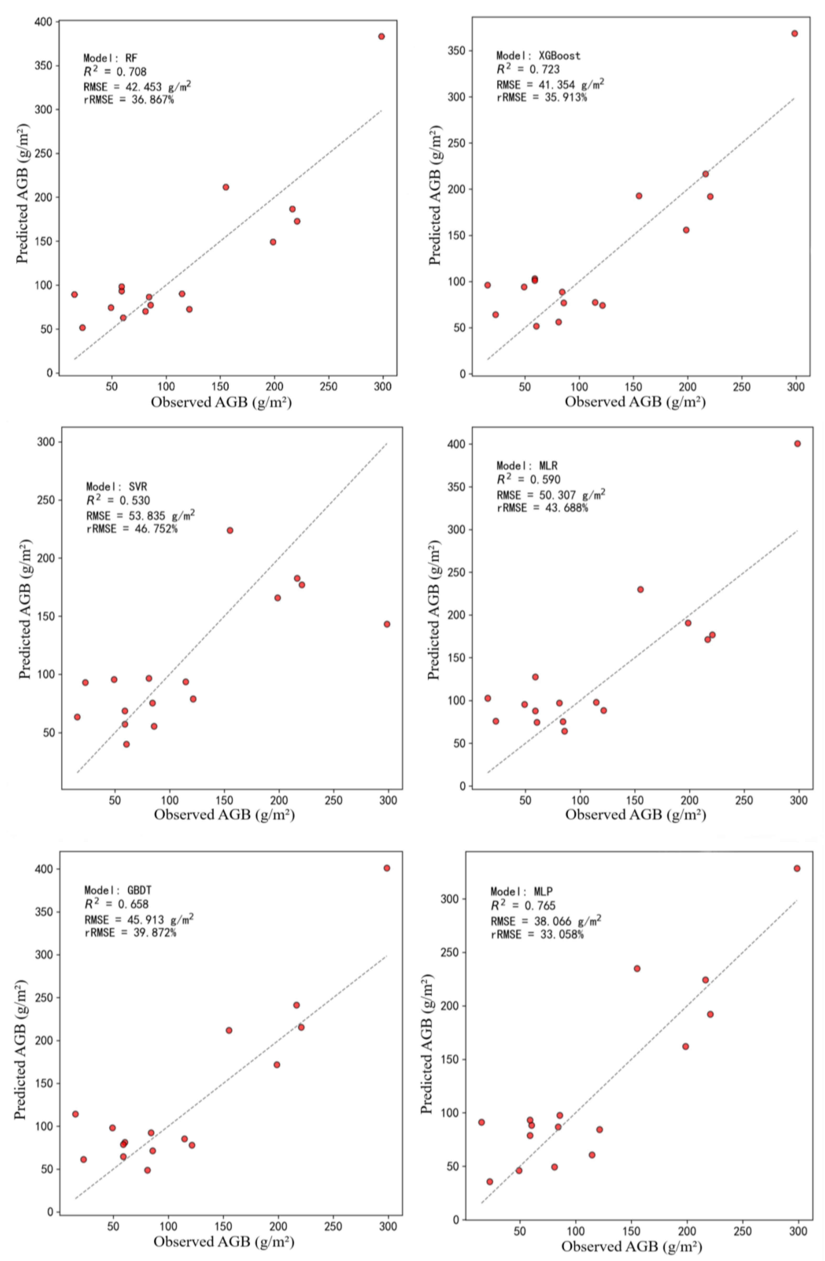
The training and testing results of traditional machine learning models and the Multilayer Perceptron (MLP) model are shown in Figure 3. The Support Vector Machine Regression (SVR) model exhibited the poorest performance (R² = 0.530, RMSE = 53.835 g/m², rRMSE = 46.752%), followed by the Multiple Linear Regression (MLR) model (R² = 0.590, RMSE = 50.307 g/m², rRMSE = 43.688%). The Gradient Boosting Decision Tree (GBDT), Random Forest Regression (RF), and Extreme Gradient Boosting (XGBoost) models demonstrated similar overall performance, with R² values ranging from 0.658 to 0.723, RMSE values from 41.354 g/m² to 45.913 g/m², and rRMSE values from 35.913% to 39.872%. The Multilayer Perceptron (MLP) model achieved the best results (R² = 0.765, RMSE = 38.066 g/m², rRMSE = 33.058%), outperforming all five traditional machine learning models across all evaluation metrics. The MLP model demonstrated significantly higher accuracy than traditional algorithms, with an R² of 0.765 compared to 0.723 for XGBoost, 0.708 for RF, and lower values for other models. To assess whether these performance differences were statistically significant, a paired t-test was conducted at α = 0.05. The results showed that the MLP’s R² was significantly higher than XGBoost (p = 0.023), RF (p = 0.018), SVR (p < 0.001), MLR (p < 0.001), and GBDT (p = 0.035). This indicates that the accuracy improvement of MLP is not due to random chance but reflects its superior ability to capture complex relationships between input variables and AGB.

5.3. Analysis of Grassland Above-Ground Biomass in the Study Area

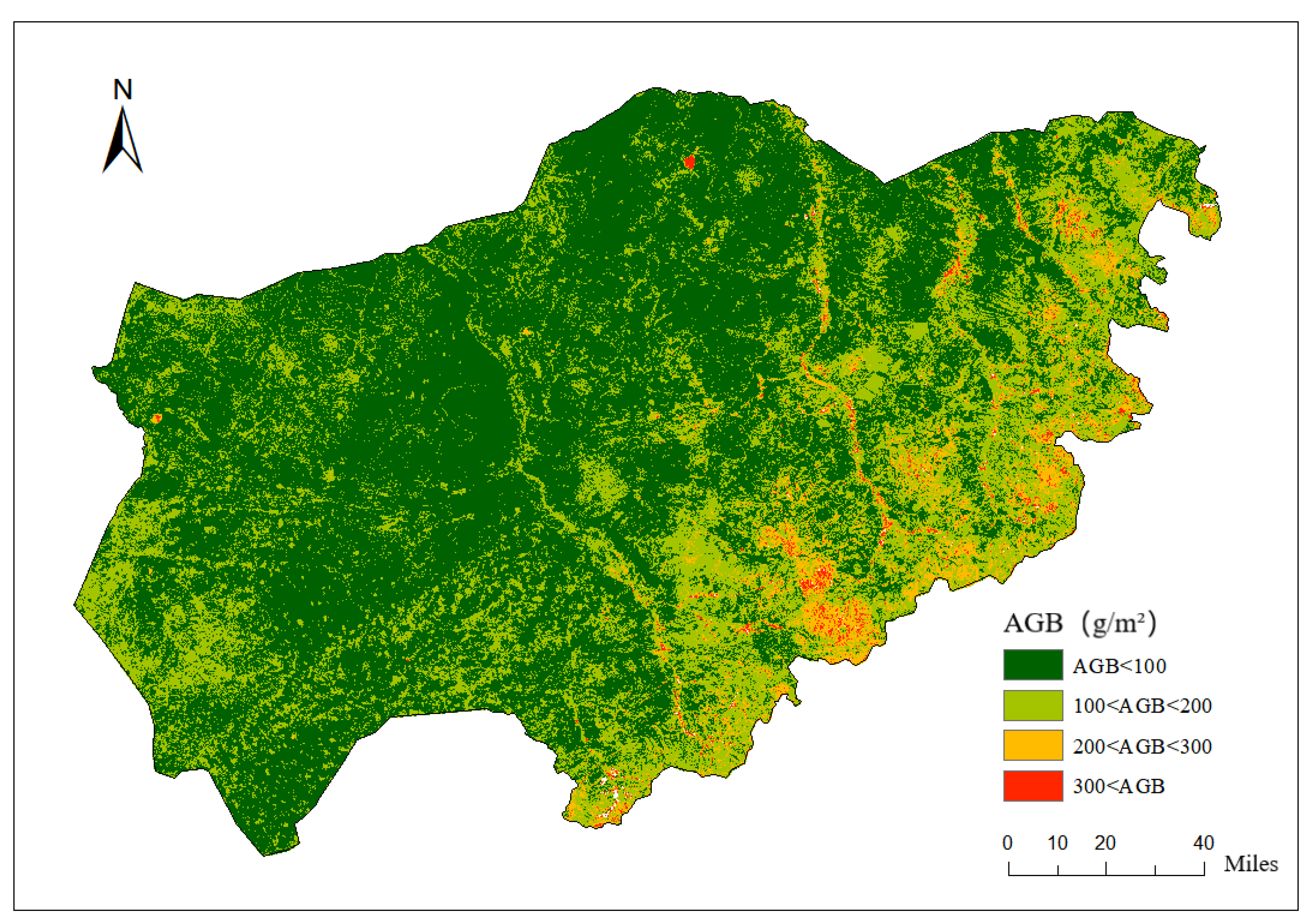
Based on the above analysis, the Multilayer Perceptron (MLP) model was selected to simulate and invert the above-ground biomass (AGB) of the entire study area (Xiwuzhumuqin Banner). ArcMap was used to map and analyze the inversion results (Figure 4). From the spatial distribution map of above-ground biomass, it is evident that there are significant spatial variations in AGB across the region.

In the northern part of the area, most of the AGB is relatively low, primarily concentrated below 100 g/m² and represented by dark green. This indicates sparse vegetation cover in this region, which is constrained by factors such as climatic conditions and soil fertility, leading to lower biomass. In the central and southern parts, AGB predominantly ranges from 100 to 200 g/m², shown in light green, indicating better vegetation coverage and relatively abundant biomass. Some areas in the south-central region exhibit AGB values between 200 and 300 g/m² (yellow) and even a few areas exceeding 300 g/m² (red), demonstrating vigorous vegetation growth. In parts of the eastern region, AGB is higher, especially in certain concentrated areas where biomass reaches 200–300 g/m² or even exceeds 300 g/m² (indicated by yellow and red). These areas have dense vegetation and abundant biomass, likely benefiting from favorable hydrothermal conditions.

Overall, AGB in Xiwuzhumuqin Banner increases gradually from the northern region to the central and southeastern regions. The northern region has relatively low biomass, while some areas in the central and southeastern regions show higher biomass, mostly concentrated between 100 and 300 g/m². This reflects a trend of increasing biomass from north to south and toward the eastern regions.

6. Discussion

Crop growth models have performed well in biomass prediction, as they integrate biological theory with computational algorithms, offering high scientific accuracy [38]. However, the reliance of these models on various data sources (such as water content, soil nutrients, etc.) and ecological theories limits their application in rapid biomass estimation [39]. In contrast, machine learning models based on the relationship between spectral reflectance or vegetation indices and biomass, with their higher simulation accuracy, robustness, and reliability, are less affected by complex environmental factors and are widely applied in biomass prediction. Machine learning models continuously optimize model parameters through feedback errors, outperforming traditional parametric models in terms of generalization ability and predictive performance, making them suitable for large-scale rapid biomass estimation [40]. The Multilayer Perceptron (MLP) model selected in this study captures the nonlinear relationships between features through its multilayer structure, better adapting to the complex variations of grassland above-ground biomass. The MLP model has demonstrated excellent performance in handling high-dimensional, nonlinear data, further improving the accuracy of biomass inversion and the model’s adaptability.

After feature selection, 14 key variables were chosen as the driving factors for the model. Among these, vegetation indices like MVI, CIg, and GNDVI show a high correlation with grassland above-ground biomass, indicating that these indices effectively reflect the biomass status of the grassland. Notably, MVI’s sensitivity to vegetation growth in arid/semi-arid environments aligns with the water limitation theory in grassland ecology, where red and shortwave infrared bands are critical for detecting water stress. This highlights how MVI captures both canopy structure and physiological status, two key indicators of grassland resilience to drought. This result is consistent with the findings of Yu Hui et al. [41]. In addition, meteorological data such as precipitation and maximum temperature are significantly positively correlated with biomass, reflecting the dynamic changes of grassland biomass under different climatic conditions. The positive correlation between soil organic carbon (SOC) and AGB (R = 0.428) reflects the soil–nutrient feedback mechanism, where SOC acts as a reservoir for plant-available nitrogen and phosphorus in semi-arid systems. This underscores the importance of soil carbon pools in sustaining grassland productivity, particularly in the eastern study area with higher SOC content (Figure 3).

In the comparison of various machine learning models, the MLP model showed the best predictive accuracy in this study, with an R² value of 0.765, RMSE of 38.066 g/m², and rRMSE of 33.058%. In contrast, other traditional machine learning models, such as Random Forest (RF) and Extreme Gradient Boosting (XGBoost), also achieved relatively high accuracy (with R² values of 0.708 and 0.723, respectively), but they were slightly less effective than MLP in fitting nonlinear complex relationships. This superiority stems from MLP’s ability to model nonlinear climate–vegetation interactions, such as the synergistic effect of precipitation and vegetation indices (e.g., NDVI). For instance, the model reveals that the positive impact of precipitation on AGB is amplified in areas with denser vegetation (higher NDVI), a phenomenon rooted in improved water-use efficiency via canopy interception. Traditional linear models (e.g., MLR) and tree-based algorithms (e.g., RF) struggle to capture such context-dependent dynamics, limiting their ecological interpretability [42]. The performance of Support Vector Regression (SVR) and Multiple Linear Regression (MLR) models was poorer, indicating limitations when handling high-dimensional and nonlinear feature data.

Additionally, this study relies on single-date Landsat imagery acquired in August, which may not fully capture seasonal variations in grassland phenology (e.g., spring growth peaks or autumn senescence). Seasonal differences in vegetation structure and spectral responses could introduce biases when applying the model to other time points. For instance, early-season biomass is more sensitive to soil moisture, while late-season biomass may be dominated by litter accumulation, both of which are not captured by the current single-date dataset. This temporal limitation highlights the need for multi-temporal imagery or time-series analysis in future studies to improve the model’s robustness across different growth stages and climatic conditions. Future studies could consider integrating higher spatial resolution remote sensing data or advanced deep learning models with multi-source data to further enhance model accuracy.

Our approach using Landsat 9 30 m imagery and MLP models offers a balance between spatial coverage and computational efficiency, differing from recent studies with alternative sensors or models. Yang et al. achieved an R² of 0.85 using UAV-based multispectral imagery at 0.5 m resolution for small grassland plots, but acknowledged challenges in scaling to regional extents due to data acquisition costs and flight time limitations. In contrast, our 30 m resolution dataset enables cost-effective mapping of thousands of square kilometers, and it is suitable for semi-arid grasslands where high-resolution surveys are logistically infeasible [43]. Li et al. applied an LSTM model to Sentinel-2 time-series data, achieving an R² of 0.79 by capturing crop phenological dynamics. While their framework excels in modeling temporal patterns, it requires ≥8 cloud-free images per season and high GPU resources. Our single-date MLP model, though limited in temporal analysis, demonstrates robustness with minimal data input, making it accessible for regions with sparse historical imagery or computational constraints [44]. Zhang et al. compared optical (Landsat-8) and SAR (Sentinel-1) data in semi-arid grasslands, finding that optical vegetation indices outperformed SAR for low-to-moderate biomass. While SAR maintained consistent performance in cloudy conditions (R² = 0.71), its sensitivity to canopy structure was weaker than optical signals in grassland ecosystems. Our optical-based approach leverages this spectral advantage to maximize accuracy in clear-sky environments, a common scenario in semi-arid regions [45].

The results of this study reveal the spatial distribution pattern of grassland above-ground biomass in Xiwuzhumuqin Banner, with biomass increasing from the northern region to the central and southeastern areas. This trend provides important references for the rational utilization and protection of grassland resources: ① This trend provides important references for grassland management. Low-biomass zones (<100 g/m², northern desert-steppe): implement strict grazing exclusion and plant drought-resistant species (e.g., Caragana microphylla) to combat desertification, as these areas have <50% vegetation cover and high soil erosion risk. High-biomass zones (>300 g/m², southeastern meadow steppe): adopt rotational grazing with a maximum stocking rate of 0.8 LU/ha (livestock units per hectare) and four-paddock rotation systems to maintain biodiversity and soil health. Medium-biomass zones (100–300 g/m², central typical steppe): use dynamic grazing management, adjusting intensity based on seasonal rainfall, with a post-grazing biomass threshold of ≥50 g/m² to sustain carbon storage. ② The strong SOC-AGB correlation suggests that soil carbon conservation—through reduced tillage and rotational grazing—is critical for maintaining grassland productivity under climate change. Degraded areas with low SOC could benefit from organic amendments to enhance nutrient cycling. ③ By integrating remote sensing and meteorological data, a real-time grassland biomass monitoring and early warning system can be established to assess risks such as climate anomalies and grassland degradation, providing technical support for ecological protection and disaster reduction.

Additionally, atmospheric effects, such as water vapor and aerosol scattering, may introduce spectral biases in the shortwave infrared (SWIR) bands used for vegetation water content retrieval. For example, undetected aerosol particles could attenuate incident radiation, leading to underestimated AGB in hazy conditions. Future studies could mitigate this by implementing advanced atmospheric correction algorithms (e.g., FLAASH or ACORN), which refine surface reflectance by removing atmospheric interference.

The 30 m spatial resolution of Landsat 9 imagery may also obscure microscale heterogeneity within grassland ecosystems, such as small-scale variations in soil moisture or grazing intensity. To address this, fusing Landsat data with higher-resolution sensors (e.g., Sentinel-2 at 10 m or UAV-based hyperspectral imagery at sub-meter scales) could capture fine-scale patterns. Alternatively, downscaling techniques like regression kriging could enhance spatial detail while retaining regional coverage.

7. Conclusions

This study underscores the transformative potential of machine learning in remote sensing for grassland ecology by demonstrating that the MLP model can effectively integrate multi-source data to uncover complex vegetation–climate interactions. For remote sensing applications, the framework establishes medium-resolution satellite imagery (e.g., Landsat 9) as a viable tool for cost-efficient regional biomass monitoring, particularly in data-scarce semi-arid regions where high-resolution surveys are logistically challenging. The identification of vegetation indices (e.g., MVI) and precipitation as key drivers provides a scientific basis for designing targeted remote sensing protocols that prioritize spectral bands sensitive to water stress and canopy structure.

In the context of grassland management, the study’s spatial biomass patterns offer actionable insights for climate-adaptive strategies. The northern low-biomass zone, linked to arid conditions and soil degradation, can be prioritized for restoration initiatives such as rainwater harvesting and drought-resistant vegetation planting. Conversely, the high-biomass southeastern region supports sustainable grazing practices with defined stocking rates and rotational systems, balancing productivity with carbon storage objectives. Moreover, the strong soil organic carbon–AGB correlation highlights the need for soil health management policies, reinforcing the role of grasslands in carbon neutrality agendas.

The specific conclusions are as follows: ① The MLP model outperformed traditional machine learning models in predicting grassland biomass, highlighting its superiority in handling nonlinear and high-dimensional data. ② Vegetation indices, meteorological data, and soil data are critical factors influencing grassland above-ground biomass. Among them, MVI, CIg, and precipitation contributed the most to inversion accuracy. ③ The results revealed spatial variations in biomass within the study area, showing lower biomass in the northern region and higher biomass in the central and southern regions. This trend offers significant references for the management of grassland ecosystems. ④ To enhance model robustness, future research should explore multi-sensor fusion strategies, such as combining Landsat 9 optical data with Sentinel-1 SAR for cloud resilience and UAV-based hyperspectral imagery (0.5 m resolution) to capture microscale heterogeneity in degraded grasslands. Regarding model architecture, Transformer-based networks could be applied to analyze multi-temporal Sentinel-2 time-series (5–10-day resolution) and model seasonal phenological dynamics, while LSTM (Long Short-Term Memory) networks may improve predictions under inter-annual climate variability (e.g., droughts). Additionally, incorporating soil moisture dynamics and grazing intensity datasets into the model could refine the representation of human–environment interactions. These advancements would enable more precise spatiotemporal AGB mapping, supporting adaptive management strategies in semi-arid ecosystems.