Article

Optimizing Power Consumption in Aquaculture Cooling Systems: A Bayesian Optimization and XGBoost Approach Under Limited Data

by
Sina Ghaemi
,
Hessam Gholmohamadi
*,†,
Amjad Anvari-Moghaddam
and
Birgitte Bak-Jensen
Department of Energy (AAU Energy), Aalborg University, 9220 Aalborg, Denmark
*
Author to whom correspondence should be addressed.
These authors contributed equally to this work.
Appl. Sci. 2025, 15(11), 6273; https://doi.org/10.3390/app15116273
Submission received: 27 April 2025 / Revised: 30 May 2025 / Accepted: 31 May 2025 / Published: 3 June 2025
(This article belongs to the Special Issue Design, Optimization and Control Strategy of Smart Grids)

Abstract

:
Driven by increased integration of renewable energy sources, the widespread decarbonization of power systems has led to energy price fluctuations that require greater adaptability and flexibility from grid users in order to maximize profits. Industrial loads equipped with flexible resources can optimize energy consumption rather than merely reacting to immediate events, thereby capitalizing on volatile energy prices. However, the absence of sufficient measured data in industrial processes limits the ability to fully harness this flexibility. To address this challenge, we presents a black-box optimization model for optimizing the energy consumption of cooling systems in the aquaculture industry using Extreme Gradient Boosting (XGBoost) and Bayesian Optimization (BO). XGBoost is employed to establish a nonlinear relationship between cooling system power consumption and available measured data. Based on this model, Bayesian Optimization with the Lower Confidence Bound (LCB) acquisition function is used to determine the optimal discharge temperature of water into breeding pools, minimizing day-ahead electricity costs. The proposed approach is validated using real-world data from a case study at the Port of Hirtshals, Denmark based on measurements from 2023. Our findings illustrate that leveraging the inherent flexibility of industrial processes can yield financial benefits while providing valuable signals for grid operators to adjust consumption behaviors through appropriate price mechanisms. Furthermore, machine learning techniques prove effective in optimizing energy consumption for industries with limited measured data, delivering accurate and practical estimations.

1. Introduction

As renewable energy sources such as wind and solar become increasingly integrated into the power system, the intermittency of the electricity supply is increasing significantly. At the same time, the shift from passive consumers to more flexible ones such as Electrical Vehicles (EVs) is adding uncertainty to electricity demand. This combination of variable supply and unpredictable demand creates challenges for power grid stability [1]. Energy flexibility is an effective solution to balance renewable energy fluctuations and ensure a stable power system. Below, energy flexibility is discussed from three perspectives: power supply, electricity demand, and energy storage.
On the demand side, flexibility has been explored across different sectors, including residential [2], commercial [3], agricultural [4], and industrial [5]. Each sector has unique electricity demand patterns and flexibility potential, requiring expert knowledge for effective management. Among these, the industrial sector has energy-intensive processes that can provide significant flexibility to the power grid.
Industrial plants are categorized into light, medium, and heavy industries. Light and medium industries are usually connected to distribution and sub-transmission networks, while heavy industries are often connected directly to the transmission network. This means that industrial energy management systems can help to support both distribution and transmission grids.
Certain industrial processes can be adjusted based on grid requirements. For example, recent studies have shown that crushers and milling machines used in cement manufacturing can change their power consumption with short advance notice [6]. Similarly, in metal smelting, electric furnaces can increase or decrease their power usage with mid-term notice, helping to help stabilize the grid [7]. Many industries also have on-site power generation (self-distributed generation), which can support the grid during power shortages. A recent study has shown that oil refineries can use their Distributed Generation (DG) units to help balance power fluctuations in the grid [8].
In recent years, the water–energy nexus has gained attention as the water industry seeks more efficient energy usage [9]. Research has suggested [10] that restructuring the agricultural sector could improve its ability to integrate more renewable energy sources. Another [11] showed that operation of irrigation pumps can be optimized to provide grid flexibility during peak demand hours, especially when crop water demand coincides with high electricity consumption periods.
Recent studies have shown that heat pumps are being used more in livestock industries, e.g., poultry farms, pig farms, and ranches [12]. These heat pumps run on electricity instead of fossil fuels, and can produce 3–5 times more heat than they use in electricity. They can also help to balance electricity demand by adjusting indoor air temperatures. Because the thermal time constant is slower than electricity, heat pumps can be turned off or down when there is not enough renewable power available on the supply side [13].
In addition to heat pumps, cooling plants are energy-intensive industrial plants in the water–energy nexus environment that can provide significant flexibility for both the heat and electricity grids [14]. In cold storage facilities such as those for meat and fish, cooling systems remove heat from the stored goods by consuming electricity. The waste heat that is removed can then be directly fed into the district heating network or used by booster heat pumps to improve the efficiency of district heating [15].
Current research on energy flexibility shows that many potential sources of flexibility in different demand sectors remain underexplored. In order to unlock this flexibility without compromising comfort or safety, expert knowledge is essential. In addition to identifying flexibility potentials, the state of the art also explores various methods for optimizing energy flexibility. In this way, depending on the availability of data and the characteristics of the energy system under study, such systems can be modeled as a white-box, grey-box, or black-box system [16]. A white-box model is used when detailed knowledge about the system’s operation and constraints is available. In such cases, the system is described using physical and mathematical equations with clearly defined constraints. These models can be solved using optimization tools such as CPLEX for linear problems [17], while solvers such as IPOPT or KNITRO are suitable for nonlinear cases [18]. For highly nonlinear or complex systems where conventional solvers may struggle, heuristic methods such as genetic algorithms or Particle Swarm Optimization (PSO) can be applied [19]. When partial knowledge of the system exists and some historical or real-time data is available, a grey-box model can be developed by combining physical insights with data-driven components. In [20], a continuous-time stochastic grey-box model was initially developed at DTU Compute and further improved at AAU Computer Science to unlock energy flexibility in buildings with multiple temperature zones. In situations where the internal characteristics of the system are largely unknown and only data are available, black-box model can be appropriate. In this approach, machine learning algorithms are used to model and optimize system behavior. Studies have shown that neural networks and Long Short-Term Memory (LSTM) models are effective in capturing and utilizing the flexibility potential of industries, especially when detailed system information is lacking [21].
This paper explores the energy flexibility potential of salmon fish breeding pools that are supported by industrial cooling plants. These cooling plants receive brine water from the sea, which is treated and then cooled or heated to maintain the required temperature range in the breeding pools. The temperature in these pools must stay within a specific range, which can be influenced by outdoor conditions. Flexibility arises from the fact that the water temperature does not need to be kept at a single fixed value but can vary within a safe range. Based on this, an intelligent control system is developed for the cooling plant to take advantage of this thermal flexibility and respond dynamically to fluctuations in electricity prices. The study is based on a real-world case located in the Port of Hirtshals in northern Denmark. Real operational data from the plant are used to create a black-box model of the system. This model is then optimized using Extreme Gradient Boosting (XGBoost) and Bayesian Optimization to improve control strategies and unlock flexibility.
The main contributions of this study are as follows:
  • Developing a black-box model for the energy consumption of a cooling plant that supplies a fish breeding pool while considering flexible temperature bounds.
  • Demonstrating the ability to unlock power-to-heat flexibility in response to dynamic electricity prices.
  • Optimizing the flexibility potential of the cooling plant using XGBoost and Bayesian Optimization supported by real-world historical data from the industrial facility.
The rest of the paper is organized as follows: Section 2 presents the methodology of the suggested approach as well as the mathematical models and formulations; Section 3 explains the case study and simulation results; finally, the last section concludes the study.

2. Methodology of Research

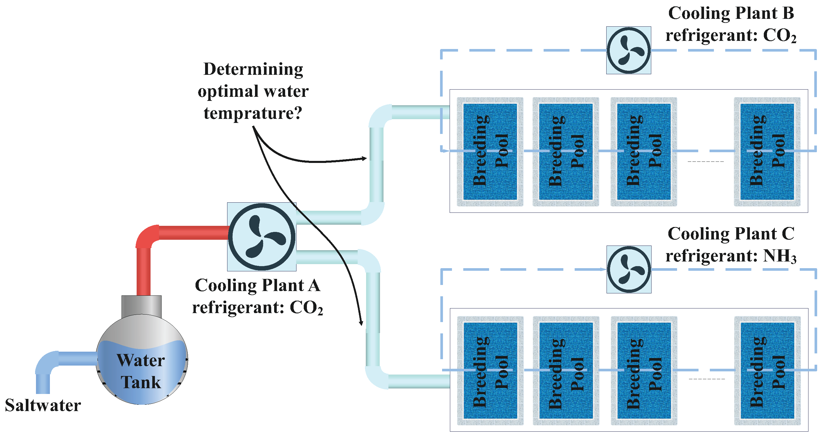
Cooling systems play a crucial role in maintaining optimal temperature of water in aquaculture breeding pools. While configurations vary across industries, each breeding pool typically has a dedicated cooling system. Several factors influence water temperature, including the temperature of discharged water, heat from machinery, fish metabolism, and ambient conditions. If these factors cause the temperature to exceed the threshold, then the cooling system must intervene. However, some aquaculture facilities also incorporate a pre-cooling system for seawater or stored water before injection into breeding pools. This process helps to reduce the energy demand of primary cooling systems, extending their lifespan and improving efficiency. This sections aims to address the minimization of the total power consumption of cooling systems in a typical aquaculture facility with an additional pre-cooling system. In fact, by optimizing the temperature of discharged water based on current data, it is possible to minimize the total energy cost of cooling systems while maintaining favorable conditions for fish production. Figure 1 presents a schematic of the system under study.
As illustrated in Figure 1, cooling plants B and C serve as the primary systems that ensure water temperatures remain within acceptable limits, while cooling plant A functions as a pre-cooling unit for the seawater intake. In this cooling system configuration, plants B and C are responsible for maintaining the water temperatures of their respective breeding pools within the acceptable range. Installation of plant A, which serves as a pre-cooling unit, helps to lower the temperature of the water before it enters the breeding pools, thereby reducing the load on the primary cooling systems. In addition, this unit enhances the overall flexibility of the facility by operating as a price-responsive system, unlike the primary units which are largely price-agnostic. In combination with the limited availability of data for assessing the flexibility of the primary cooling systems, these characteristics underscore the importance of optimizing the operation of the precooling unit. The following subsections outline the mathematical formulation of the model, followed by a discussion on data limitations and the challenges of acquiring certain operational parameters. To address these constraints, this study explores how machine learning techniques can enhance decision-making around determining the optimal water discharge temperature for breeding pools.

2.1. Mathematical Model

As discussed earlier, the main objective function is to minimize the total energy cost of cooling systems within a typical day based on the forecasted electricity prices. This can be formulated as follows:
min F = t = 1 24 ( π t e l e c + π O & M ) [ P A t C S + P B t C S + P C t C S ]
where π t e l e c , π O & M , P A t C S , P B t C S , and  P C t C S show the electricity price, operating cost of the cooling systems, and electric power consumption of the cooling system A, B, and C, respectively. This optimization model incorporates key technical constraints, including the calculation of electrical power consumption for the pre-cooling system (plant A) and the primary cooling systems (plants B and C) as well as limitations related to maintaining the water temperature in the breeding pools within acceptable bounds. In relation to the precooling system, the amount of heat power absorbed from the water intake from the water tank can be calculated using Equation (2):
Q t A , C S = m H 2 O C H 2 O ( T t i n T t o u t )
where m H 2 O , C H 2 O , T t i n , and  T t o u t stand for the mass flow rate of water intake from the tank (m3/h), specific heat capacity of water (4.186 MJ/m3C), water intake temperature from seawater, and temperature of the water discharged into the breeding pools, respectively. Then, based on the Coefficient Of Performance (COP) of this system, its electrical power consumption at time t is calculated as follows:
P j , t C S = Q t A , C S C O P A j [ A ]
where C O P A stands for the COP of the pre-cooling system. There is a technical constraint that concerns the extent to which the pre-cooling system can reduce the water temperature. This reduction is limited by the system’s capacity along with other operational considerations such as equipment longevity and the need to avoid excessive cooling. As a result, the temperature of the discharged water must remain within a predefined acceptable range, represented by the following constraint:
T t m i n T t o u t T t i n
where T t m i n represents the minimum allowable temperature of the water discharged into the breeding pool. In addition, the water temperature of the each breeding pool must be kept within the acceptable range regardless of the temperature of the discharging water, and the primary cooling systems associated with each of them must cool the water when the water temperature exceeds the threshold. Therefore, based on the temperature requirements of the breeding pools, the temperature of the water T p o o l in a typical breeding pool (e.g., k) must be less than the prespecified value T S P . , as follows:
T k , t p o o l T S P .
As mentioned, the primary CO 2 and ammonia cooling systems (those highlighted by plant B and C in Figure 1) are designed to lower the temperatures of their respective pools when exceeding the specific threshold, which can happen due to fish metabolism and machinery processes as well as to discharges from the water tank. Hence, the temperature of the k th breeding pool at the next time step can be calculated as follows:
T k , t + 1 p o o l = T k , t p o o l ( V k , t p o o l Q i n , t p o o l ) + T i n , t p o o l Q i n , t p o o l Δ t + Q f i s h , t + Q m a c h i n e r y , t V k , t p o o l
where T k , t + 1 p o o l , T k , t p o o l , V k , t p o o l , Q i n , t p o o l , Q f i s h , t , and Q m a c h i n e r y , t refer to the next temperature of the breeding pool cooled by the k th cooling system, the current temperature of the breeding pool, the total volume of the breeding pool, the water inflow rate, the heat produced from fish metabolism, and the heat produced by machinery processes, respectively. In this equation, T i n , t p o o l is the same as the temperature of the water cooled by means of the pre-cooling system ( T t o u t ). Finally, the amount of active power required for cooling of the breeding pool ( P k , t r e q u i r e d ) can be calculated using Equation (7):
P j , t r e q u i r e d = ( T k , t + 1 p o o l T S P . ) V k , t p o o l C H 2 O Δ t T j , t + 1 p o o l T S P , 0 T j , t + 1 p o o l T S P .
Finally, the electricity power consumed by primary cooling systems can be calculated as follows:
P j , t C S = P j , t r e q u i r e d C O P j : j [ B , C ] .
As discussed, the primary objective is to minimize the operating cost of the cooling systems by responding intelligently to dynamic electricity prices throughout the day while ensuring that the water temperature in the breeding pools remains below a predefined threshold and avoiding deep pre-cooling. Hence, the corresponding optimization problem along with its technical constraints can be summarized as follows:
Model CS Objective Function: Equation   ( 1 ) , Breeding pools requirements: Equations   ( 4 )–( 6 ) , Power consumption of preecooling unit: Equations   ( 2 )–( 3 ) , Power consumption of primary cooling systems: Equations   ( 7 )–( 8 ) .

2.2. Solution Method Under Limited Available Data

As declared above, this study aims to minimize the total energy consumption of three cooling plants responsible for maintaining optimal water temperatures in breeding pools. Developing an exact mathematical model requires detailed data on cooling plant characteristics, breeding pool volumes, hourly fish biomass, and excess heat from machinery. However, collecting these data can be time-consuming and in certain cases impractical. Typically, installed sensors measure power consumption and discharge water temperature but do not capture the heat generated by machinery or fish metabolism, which are often difficult or impossible to quantify. To overcome these limitations, this study leverages machine learning techniques to provide more accurate energy consumption estimations based on available data. To achieve this, the power consumption of each primary cooling plant (B and C in Figure 1), each corresponding to a specific breeding pool, is first predicted using the Extreme Gradient Boosting (XGBoost) algorithm [22] leveraging various input features. Subsequently, Bayesian Optimization [23] is applied to determine the optimal water inlet temperature for the breeding pools while minimizing energy consumption, as per the objective function in Equation (1). It is worth mentioning that the key consideration in selecting the aforementioned techniques was the direct applicability of the developed model in industrial contexts, particularly within the aquaculture sector. In such settings, industries often prefer established and interpretable techniques over newer or more complex alternatives. Moreover, selection of the employed methods was not made in isolation, being carefully reviewed and validated by our industrial partners to ensure that the chosen techniques are both understandable and feasible for implementation and can enhance system flexibility within their operational environments. This decision reflects a necessary tradeoff between academic novelty and industrial applicability. The following subsections provide a detailed overview of these techniques.

2.2.1. The Developed XGBoost Algorithm for Power Consumption Prediction

The main objective of this algorithm is to establish the true relationship between the input features and the target output by using an ensemble model composed of multiple regression trees. This model is formulated as follows:
y ^ i = k = 1 K f k ( X i )
where X refers to the vector of the input features, y stands for the target output (in our case, the power consumption of a typical cooling plant), and f demonstrates the k th regression trees. In addition, K shows the number of trees in the developed ensemble. The training objective function of this algorithm consists of two terms: one that minimizes the prediction error and another that prevents overfitting. It is formulated in Equation (10):
F = i = 1 n l ( y i , y ^ i ) + k = 1 K χ f k
where l ( . ) and χ refer to the loss function and regularization term, respectively, which can be structured as follows:
l ( y i , y ^ i ) = ( y i y ^ i ) 2
χ f k = γ T + 1 2 λ j = 1 T ω j 2
where T shows the number of leaves on each tree, ω j refers to the weight associated with the j th leaf, and  γ and λ are hyperparameters for controlling the strength of regularization. The regularization term is considered in order to avoid overfitting by diminishing the model complexity. In this technique, the ensemble is constructed incrementally; in the k th iteration, the prediction value is determined using Equation (9), with a new tree f added to the training objective function as follows:
F ( k ) = i = 1 n l ( y i , y ^ i k 1 , f k ( X i ) ) + χ f k .
A second-order Taylor expansion is used to approximate the loss function in order to optimize the objective function. It can be formulated as follows:
l ( y i , y ^ i k 1 , f k ( X i ) ) l ( y i , y ^ i k 1 ) + g i f k ( X i ) + 1 2 h i f k ( X i ) 2
where
g i = l ( y i , y ^ i ) y ^ i | y ^ i = y ^ i k 1 ,
h i = 2 l ( y i , y ^ i ) 2 y ^ i | y ^ i = y ^ i k 1 .
The simplified objective function is then derived by substituting the approximated loss function with the initial function while omitting constant parameters, as follows:
F ( k ) = i n [ g i f k ( X i ) + 1 2 h i f k ( X i ) 2 ] + χ f k .
This simplified objective function is minimized based on the structure and leaf values of the new tree. In this model, each regression tree splits the feature space into regions (R), then attributes a weight ( ω ) to all instances within each region. The optimal weight can be computed using Equation (18):
ω j * = i R j g i i R j h i + Λ .
Finally, Algorithm 1 demonstrates the mathematical procedure of the proposed model.
In this approach, optimizing input features is known to be vital for improving the accuracy of power consumption predictions based on available data. In the proposed model, three feature categories are considered for forecasting the power consumption of a specific cooling plant at time t.
Algorithm 1 Steps of the Proposed Solution Technique
  • Input: Data and initial prediction (e.g., mean of y)
  • Output: Optimal solution y ^
  • procedure  OptimalSolution
  •     Initialization: Set initial prediction
  •     for  k = 1  to K do
  •         Compute gradients g i and Hessians h i based on current predictions
  •         Fit regression tree f k to these gradients
  •            Determine optimal splits maximizing gain (with regularization)
  •            Assign a weight to each leaf (using the closed-form solution)
  •         Update model: y ^ i ( k ) y ^ i ( k 1 ) + f k ( X i )
  •     end for
  •     Final Prediction:  y ^ i k = 1 K f k ( X i )
  • end procedure
Time-Based Features:
Hour of Day: Captures diurnal consumption patterns.
Season: Accounts for seasonal variations.
Temperature-Based Features:
T t i n : Represents the water intake temperature, a critical factor that significantly affects power consumption. During the training process, this parameter is modeled using two input features: Temp in low and Temp in high . The former captures how much the water temperature falls below the threshold, while the latter reflects the amount by which it exceeds the threshold.
Lagged Feature:
P t C O 2 : Previous Hour Power Consumption: Incorporates the previous hour’s power consumption to capture temporal dependencies and inertia in power usage.
As can be seen, each feature set captures distinct consumption patterns, and combining them with the gradient boosting framework of the XGBoost algorithm enhances predictive performance.

2.2.2. Bayesian Optimization Problem

As discussed in previous sections, our model integrates the XGBoost algorithm to predict the power consumption of two primary cooling systems near the breeding pools. This adds complexity to the optimization function, making it a computationally expensive, black-box, and derivative-free problem. In such cases, the Bayesian Optimization (BO) machine learning approach provides an efficient solution by using a surrogate model to approximate the objective function. This approach is particularly effective under the following circumstances:
Low-Dimensional Decision Variables: In our model, the decision variable dimension is 24, as we aim to determine the optimal water temperature entering the breeding pools.
Simple Feasible Set: The decision variables must be constrained within a defined range, such as a hyper-rectangle x m i n x t x m a x . In this case, the optimal temperature is bounded as T t m i n T t o u t T t i n .
Continuity of the Objective Function: The objective function should be continuous in order to allow for effective approximation using Gaussian Processes (GP). Our objective function meets this criterion, as it seeks to minimize total energy consumption across the three cooling systems used in the aquaculture industry (see Equation (1)).
Indeed, the selected approach performs well in low-data black-box scenarios that are expensive-to-evaluate. It offers intuitive control over the exploration–exploitation tradeoff and provides transparent uncertainty estimates that are trusted by industrial partners. Its lightweight and CPU-efficient implementation along with minimal need for hyperparameter tuning make it significantly more practical for deployment in factory IT environments compared to data-intensive neural networks.
In the first step of BO, a prior distribution is assigned to the unknown objective function using a Gaussian Process (GP). Gaussian Processes are flexible non-parametric probabilistic models that are ideal for approximating complex and expensive-to-evaluate functions. The main strength of GPs lies in their ability to provide a probabilistic measure of uncertainty in predictions, balancing exploration (sampling in uncertain regions) with exploitation (sampling promising regions). A GP is characterized by a mean function and a covariance function, defined as follows:
f ( x ) GP m ( x ) , k ( x , x )
where m ( x ) is typically chosen as a simple mean function (often zero) and  k ( x , x ) is the covariance function (kernel) that encodes assumptions regarding the smoothness and continuity of the function. In this work, the Matern covariance is considered as the covariance function, formulated as follows:
C ν ( d ) = σ 2 2 1 ν Γ ( ν ) ( ( 2 ν ) d ρ ) ν K ν ( ( 2 ν ) d ρ )
where d is the Euclidean distance between points, ν is a positive smoothness parameter, σ 2 controls the function variance, ρ is the length-scale parameter governing the correlation between points, and  K ν denotes the modified Bessel function of the second kind. Given observed data points ( x i , y i ) i = 1 n in which y i = f ( x i ) , the GP posterior predictive distribution at any new candidate point x is explicitly updated as follows:
f ( x ) D n N μ n ( x ) , σ n 2 ( x )
with the posterior mean μ n ( x ) and variance σ n 2 ( x ) computed as follows:
μ n ( x ) = m ( x ) + k ( x , X n ) [ K ( X n , X n ) + σ ϵ 2 I ] 1 ( y n m ( X n ) ) ,
σ n 2 ( x ) = k ( x , x ) k ( x , X n ) [ K ( X n , X n ) + σ ϵ 2 I ] 1 k ( X n , x ) ,
where X n denotes the set of observed points, y n denotes the corresponding observations, K ( X n , X n ) is the covariance matrix of the observed data, k ( x , X n ) represents the covariance between new and observed points, and  σ ϵ 2 stands for the observation noise. This model includes an acquisition function that needs to be maximized in order to find the next point. In our study, we consider the Lower Confidence Bound (LCB) for this purpose, as follows:
α L C B ( x ) = μ n ( x ) κ σ n ( x )
where κ is a parameter for balancing exploration and exploitation. A theoretically justified selection for this value is as follows:
κ = 2 log π 2 n 2 6 δ .
The next evaluation point is determined by solving the following optimization problem:
x n + 1 = argmin x A α L C B ( x )
where the feasible domain A incorporates all the operational and physical constraints, such as allowable temperature limits and inlet–outlet temperature relationships. As seen above, this approach provides significant advantages over conventional optimization methods, particularly through the use of Gaussian Processes and the LCB acquisition function. Specifically, it requires fewer function evaluations, making it highly suitable for expensive-to-evaluate functions, can naturally manage uncertainty and noisy observations, and explicitly balances exploration and exploitation to efficiently explore the solution space. Algorithm 2 clearly summarizes this iterative optimization process.
Algorithm 2 Steps of Bayesian Optimization
  • Step 1: Precede f with a Gussian process
  • Step 2: Observe f at n 0 points based on the initial space-filling design.
  • Step 3: Iterative process
  • while  n N : do
  •       Estimation of the posterior probability distribution on f considering the available information
  •       Calculation of the acquisition function based on the current posterior probability distribution
  •       Estimation of f ( X )
  •     n = n + 1
  • end while
  • Final Prediction: the best observed X * is taken as the optimal schedule T o u t * = argmin f ( x )

3. Simulation Results

The effectiveness of the proposed optimization model was evaluated in a real aquaculture industry at the Port of Hirtshals in Denmark. The facility features three cooling systems. Saltwater is drawn in through a water tank that is regularly refilled by another facility. One of the newly installed cooling systems is responsible for pre-cooling of the water prior to discharge into the breeding pools. Additionally, each breeding pool is equipped with a primary cooling system that lowers the water temperature and keeps it within acceptable bounds. Technical and economic information regarding this industry can be found in Table 1.
Figure 2 illustrates the hourly heatmap of the saltwater temperature intake from the water tank in 2023.
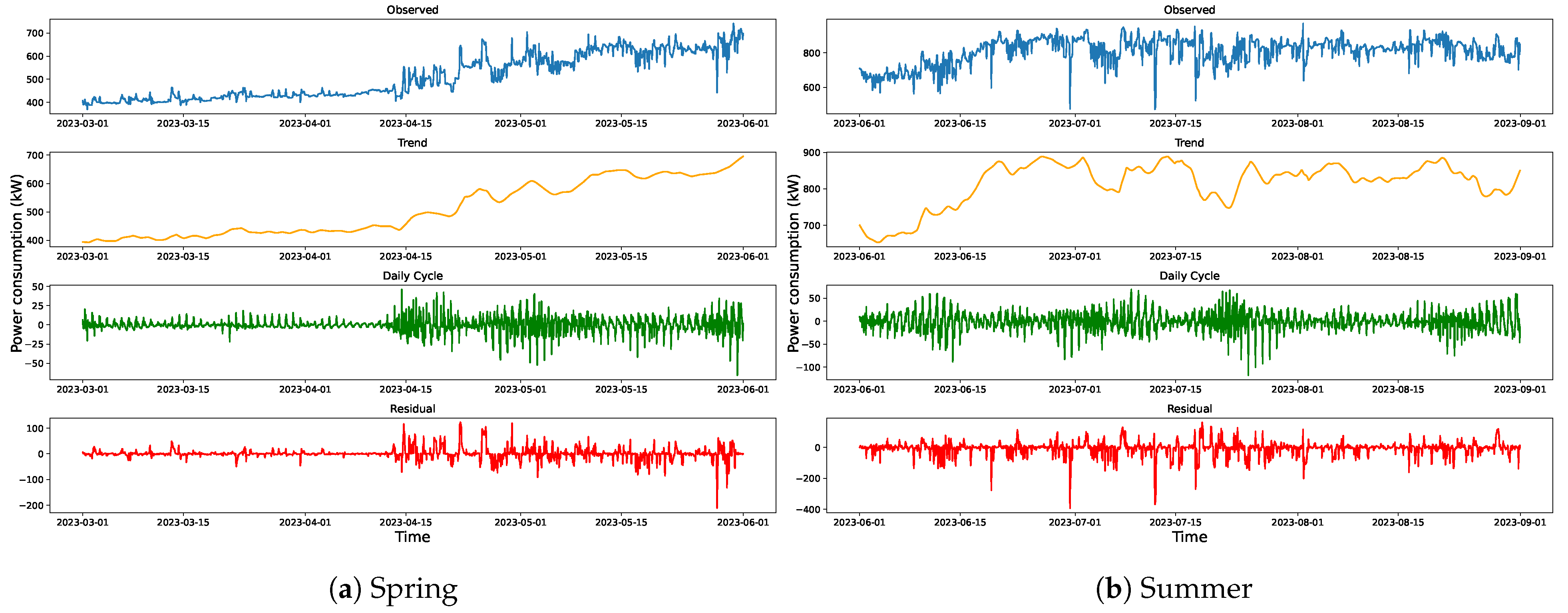
As expected, as summer approaches, the temperature of the water rises; closer to winter, the colder water reduces the need for operation of the cooling systems. In the industry under study, two cooling systems are responsible for reducing the water temperature, while the third system is used for pre-cooling. The power consumption of these systems was measured in different hours from the year 2023. Figure 3 demonstrates the seasonal-trend decomposition of the power consumption of the ammonia cooling system using the Loess method for two seasons, namely, spring and summer.
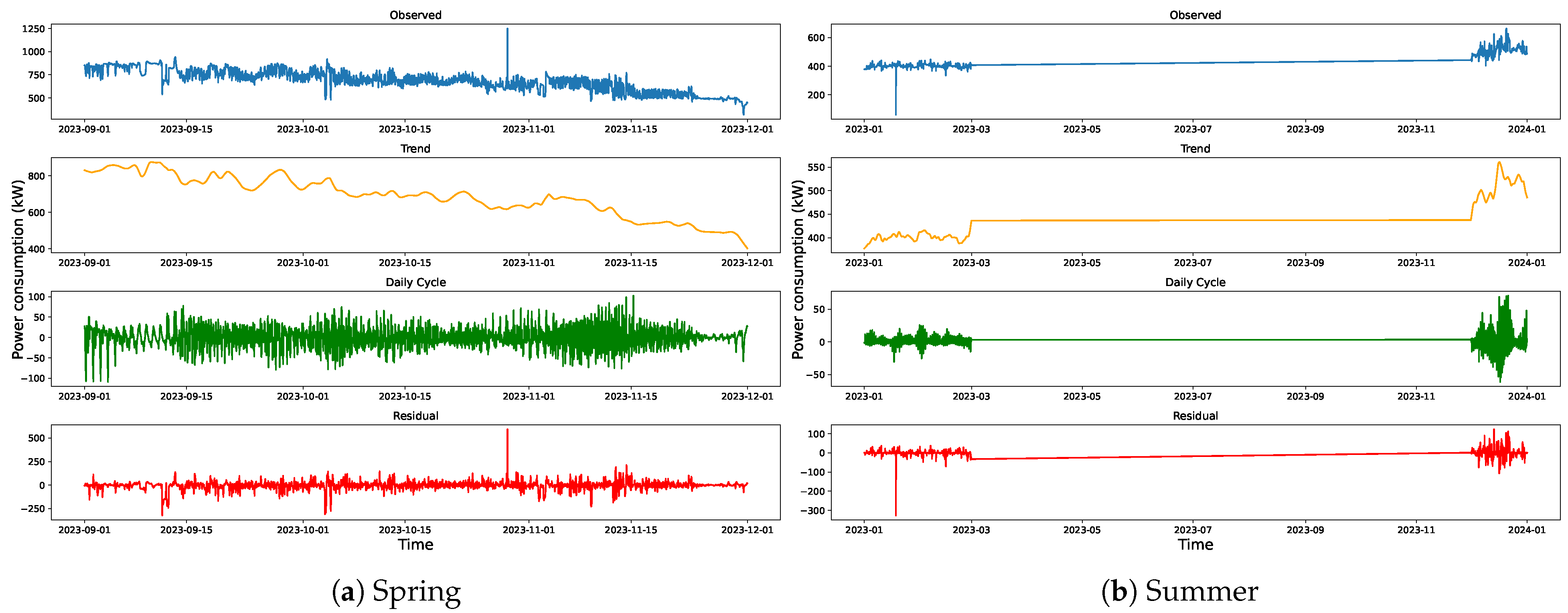
According to this technique, the observed data were decomposed into three components: trend, daily cycle, and residual. The trend component graph illustrates the long-term progression of power consumption by eliminating short-term fluctuations. As shown in the spring graph, power consumption increases as summer approaches, likely due to higher saltwater temperatures. However, fluctuations in the trend during summer can be attributed to variations in water temperature throughout the season, and the maximum power consumption reaches nearly 900 kW. The daily cycle component extracts the portion of the power consumption data that repeats every 24 h, helping to identify the hours when peaks and valleys occur. Finally, the residual component captures what remains after removing both the trend and daily cycle from the observed data, highlighting potential outliers, measurement errors, or unexpected events impacting the cooling system. It is noteworthy to mention that significant residual values during certain hours suggest that these periods warrant further investigation. A similar decomposition analysis was applied to the power consumption of this unit in autumn and winter, with the results shown in Figure 4.
In contrast to the summer trend, the autumn trend component shows a reduction in the cooling system’s power consumption as winter approaches. Moreover, the residual values are insignificant for most hours, which improves the prediction of power consumption based on the trend and daily cycle patterns. Furthermore, when examining the decomposition results for winter, we observe that for most hours the power consumption is zero, indicating that during those periods the water temperature is below a specific threshold and the cooling system does not need to operate. After addressing the seasonal-trend decomposition for the ammonia cooling system, it should be mentioned that the decomposition residuals average 44 kW and 47 kW in summer and fall, respectively, with a Coefficient of Variation (CV) close to 6%, compared to 19 kW and 21 kW with a CV near 4% in winter and spring. The increase in residuals during the warmer seasons can be attributed to two key factors: (1) higher condensing temperatures, and (2) more frequent fish-handling activities, which result in short but intense bursts of metabolic heat. These results suggest that the residual variability is primarily driven by predictable exogenous events rather than model mis-specification.
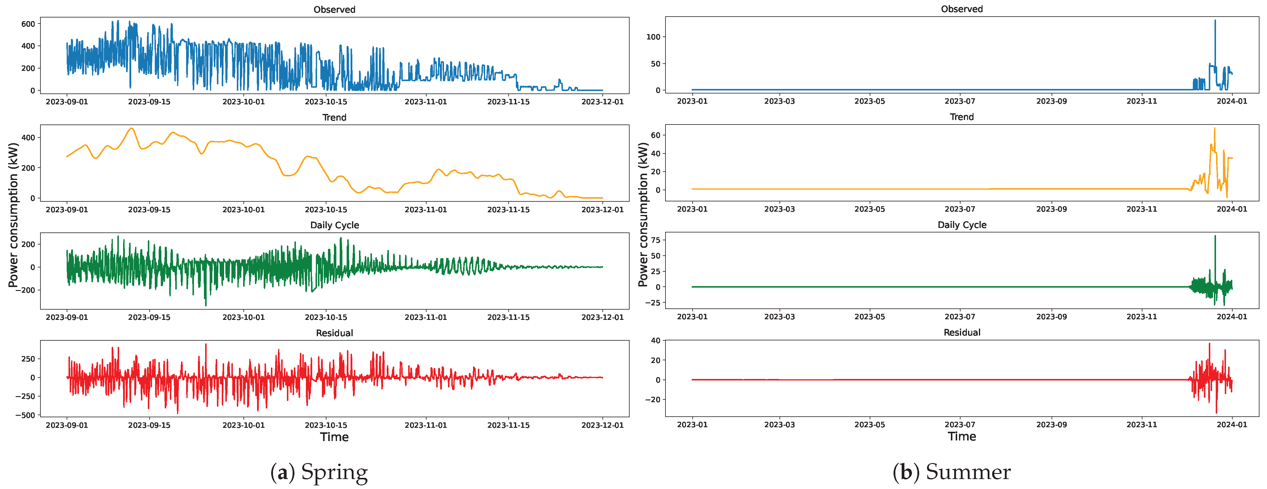
A similar analysis was performed for the CO2 cooling system, and the decomposition of its power consumption in spring and summer are provided in Figure 5.
The trend component for spring shows that for most hours of the season the cooling system remains in standby mode with minimal power usage, as the breeding pool’s water temperature stays below the threshold; however, in the summer greater fluctuations in water temperature lead to more variation in the trend component. Additionally, the high variability in the residual component suggests the influence of other significant factors such as fish metabolism, unexpected events, or increased machinery heat production, making the system’s prediction more challenging. Figure 6 presents the same analysis for the following two seasons.
It is apparent from Figure 6 that as winter approaches and water temperatures decrease, the power consumption of this unit declines, following a predictable daily cycle; however, the same challenge observed in the previous season persists. High residual values indicate the presence of other influential factors affecting the cooling system’s operation. Additionally, similar to the ammonia cooling system in winter, this cooling system operates in standby mode with minimal power consumption due to the lower saltwater temperature. For the CO2 cascade loop, the residual standard deviation reaches 86 kW in summer and 100 kW in fall, with corresponding CVs of 35% and 52%, respectively. This elevated variability can be explained from two perspectives: first, irregular bursts of metabolic or machinery heat from warm-season activities may contribute to erratic load spikes; second, the trans-critical CO2 compressor operates near its pressure limit during these periods, making it more sensitive to brief suction-pressure disturbances. In contrast, during winter and spring the system is largely idle and the mean power consumption drops below 10 kW, meaning that even minor startup or defrost pulses result in a CV exceeding 50%.
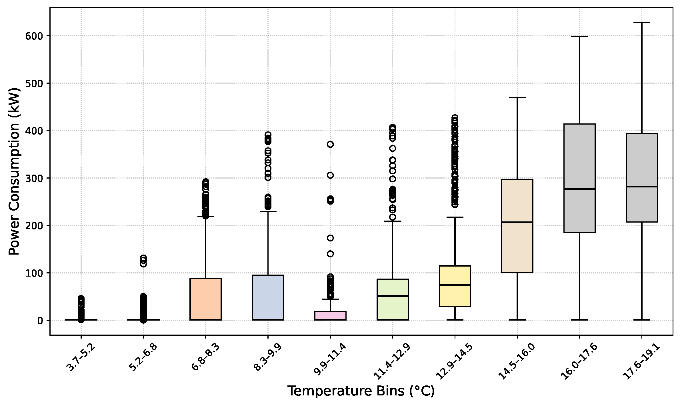
As reviewed in the decomposition analysis, the most prominent factor in the power consumption of the cooling systems associated with breeding pools is the temperature of the water discharged to these pools. In this regard, Figure 7 categorizes the power consumption of the ammonia cooling systems based on water temperature bins.
As expected, higher water temperatures correlate with increased power consumption in the cooling system. However, the presence of outliers in certain bins indicates deviations from the expected pattern, suggesting unusual events that warrant further investigation of the recorded data. A similar analysis was conducted for the other cooling system. Figure 8 shows the power consumption distribution across different temperature bins for the CO2 cooling system.
Again, higher temperatures lead to increased power consumption; however, the significant variability at higher temperatures and the presence of outliers at lower temperatures suggest additional hidden factors influencing the unit’s operation. This complexity makes predicting power consumption more challenging. According to our deep review of the power consumption of the two primary cooling systems, it can be concluded that due to higher values for the residual components in certain hours, finding the accurate pattern for these systems is demanding and requires more information. However, leveraging the strengths of XGBoost can help to find the nonlinear relation between the input features and the power consumption of the cooling systems, covering the aforementioned challenge. First, Grid Search Optimization is used to find the optimal hyperparameters of this technique, according to which the best fit can be estimated. Figure 9 shows the actual and optimized XGBoost predicted power consumption of the ammonia cooling system for the test data.
The subfigures demonstrate that the optimized XGBoost model accurately predicts the cooling system’s power consumption by leveraging the three selected feature types, effectively capturing its consumption patterns. In this regard, Table 2 compares the model’s performance against existing methods using various evaluation metrics.
As shown in Table 2, the proposed XGBoost model outperforms existing techniques across three error evaluation metrics. Additionally, its high R 2 value indicates strong accuracy despite variability in observed consumption data. A similar analysis was conducted for the other cooling system, and Figure 10 compares the predicted power consumption to the actual test data.
Despite the high variability in power consumption and the presence of outliers, the proposed model successfully captures the unit’s consumption pattern. Table 3 presents the model’s performance evaluation using various error criteria.
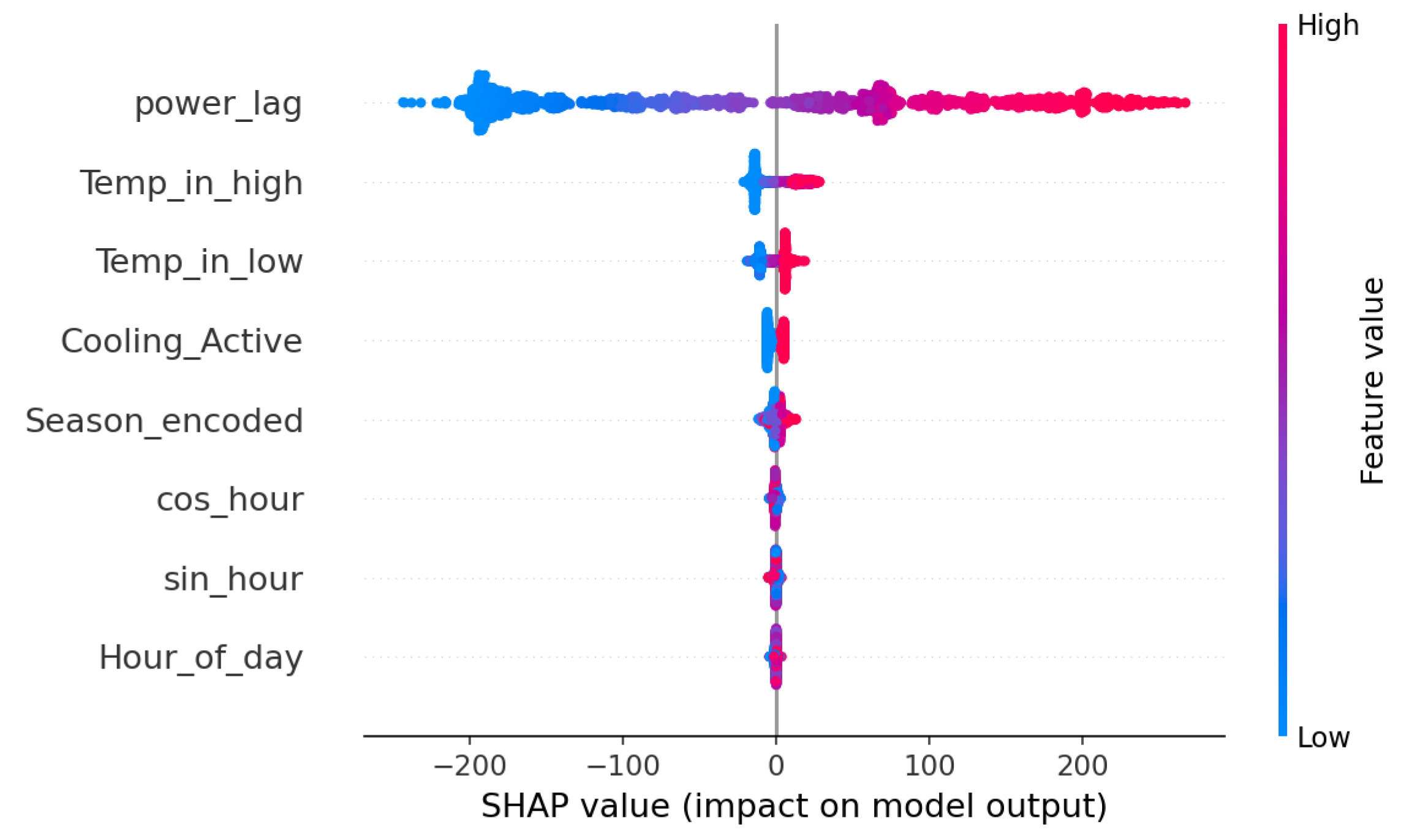
Despite high residual variability, Table 3 illustrates that the proposed model surpasses existing solutions in predicting the cooling system’s power consumption. Furthermore, the high R 2 value confirms the model’s accuracy across a wide range of data variations. To assess the explainability of the developed XGBoost model, SHAP values for the ammonia cooling system were calculated using the test data. These values visually summarize the feature importance across predictions, and are presented in Figure 11.
As shown in Figure 11, the previous hour’s power consumption emerges as the most influential feature. If the cooling system consumed a large amount of power in the prior hour, the model assumes inertia and predicts similarly high consumption for the current hour. In addition, the temperature of the water discharged into the breeding pool is another key driver; each additional degree above 12 °C typically increases power consumption by several kilowatts. The tight and mostly positive SHAP distribution supports the intuitive linear relationship between thermal load and compressor effort. Interestingly, when the water temperature is significantly below the threshold value (represented by Temp_in_low in Figure 11), it pulls the power prediction downward, suggesting reduced energy demand. However, temperatures close to the threshold do not significantly affect the forecast on their own. A binary indicator capturing the system’s operational status is also included. When the system is active (indicator = 1, shown in red), the SHAP values are generally positive, whereas inactive states (indicator = 0, shown in blue) correspond to near-zero or slightly negative values. However, this flag is less impactful than the actual temperature deviation. Seasonal effects have a moderate influence. Higher numeric values corresponding to summer and autumn yield slightly positive SHAP values, indicating a small expected increase in power consumption during warmer months after accounting for real-time temperature. Finally, circadian patterns contribute subtle refinements to the forecast, typically in the range of ±10 kW. Their centered distribution implies that these features help to fine-tune predictions rather than drive them. Indeed, the SHAP analysis suggests that this unit’s operation is primarily reactive, focused on maintaining water temperature rather than on strategically aligned with dynamic electricity pricing. This behavior highlights the system’s role in thermal regulation rather than economic optimization. A similar analysis is provided for the other main cooling system with CO2 refrigerant, which can be found in Figure 12.
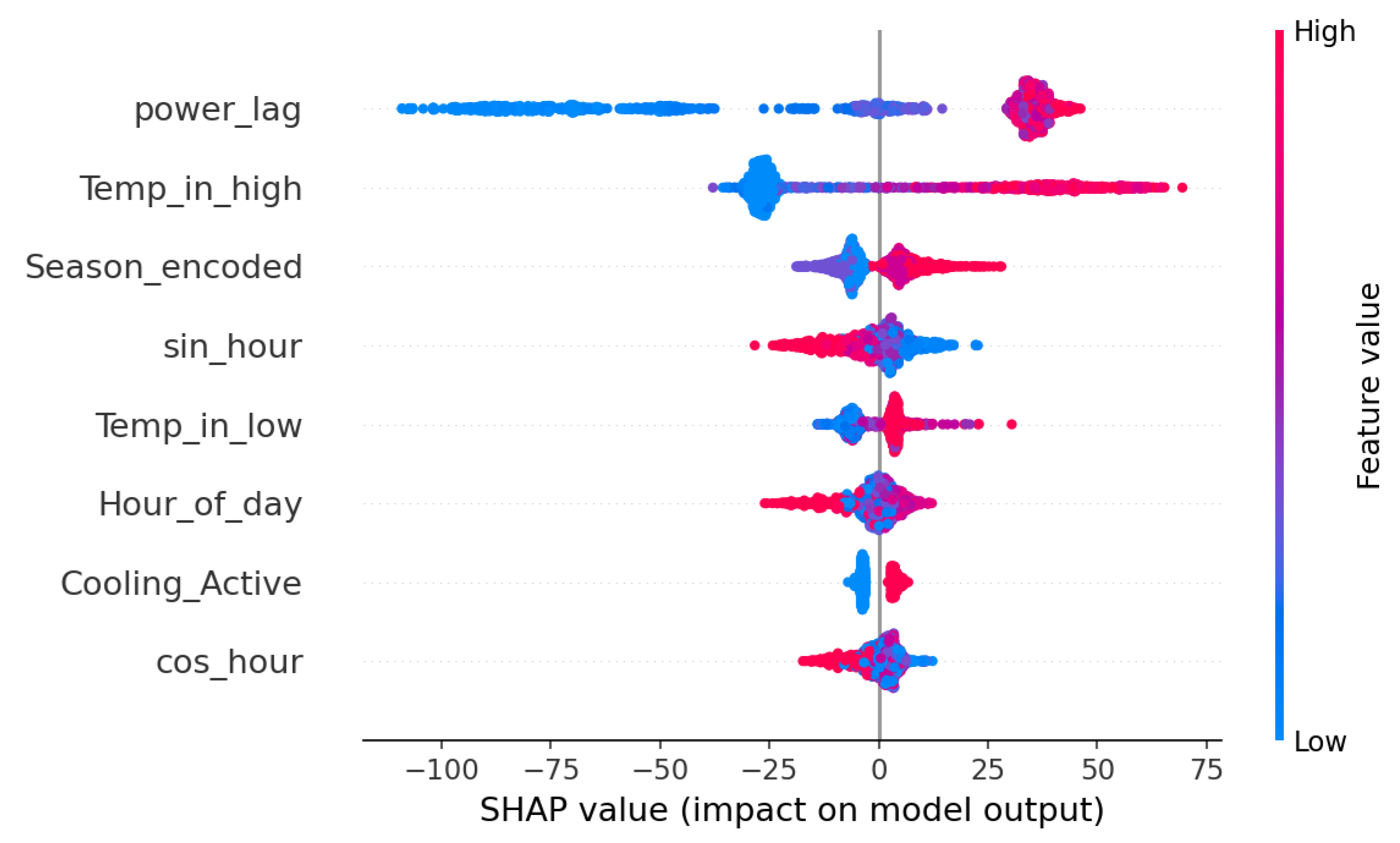
Similar to the previous cooling system, the previous hour’s power consumption plays a dominant role in predicting the current hour’s usage. This single feature effectively summarizes various hidden factors such as heat load, set-points, defrost cycles, door openings, and brief weather anomalies that were active during the previous hour. Because thermal energy scatters slowly, a high load in the previous hour remains the strongest predictor of current consumption. As a result, the model relies on this input more heavily than any other. From an operational standpoint, this implies that smoothing spikes or pre-cooling during low-price periods not only delivers immediate savings but also sets the system into a lower operational state, potentially reducing the next hour’s demand by tens of kilowatts. As expected, each additional degree above 12 °C contributes significantly to power consumption, increasing demand by tens of kilowatts. Unlike the earlier system, this unit exhibits higher power consumption (approximately 20 kW more) even after controlling for the actual water temperature during summer and autumn hours. This pattern is likely influenced by additional seasonal factors such as humidity, occupancy levels, or adjusted set-points. Finally, the daily rhythm contributes a moderate influence on consumption patterns, while the binary variable indicating whether the system is active has the least impact among all features.
As seen, the two most influential factors in predicting the power consumption of the cooling systems are the previous hour’s power consumption and the temperature of the water discharged into the breeding pools. Therefore, it is essential to examine the conditions under which the maximum prediction error occurs across different ranges of these two variables. The error is defined as the difference between the predicted and actual values ( E r r o r = P r e d i c t e d A c t u a l ). Figure 13 illustrates the distribution of prediction errors across various combinations of these two key factors for each cooling system.
Upon closer inspection of the sub-figures, it is evident that the prediction errors in both models generally remain within an acceptable range across most combinations of input variables. However, the largest errors occur at the extreme points. In the sub-figure related to the ammonia cooling system, these extremes correspond to situations where the the previous hour’s power consumption is particularly high. Similarly, the next sub-figure related to the CO2 cooling system shows that the highest errors arise when there is very high power consumption in the previous hour, especially when accompanied by elevated water temperatures.
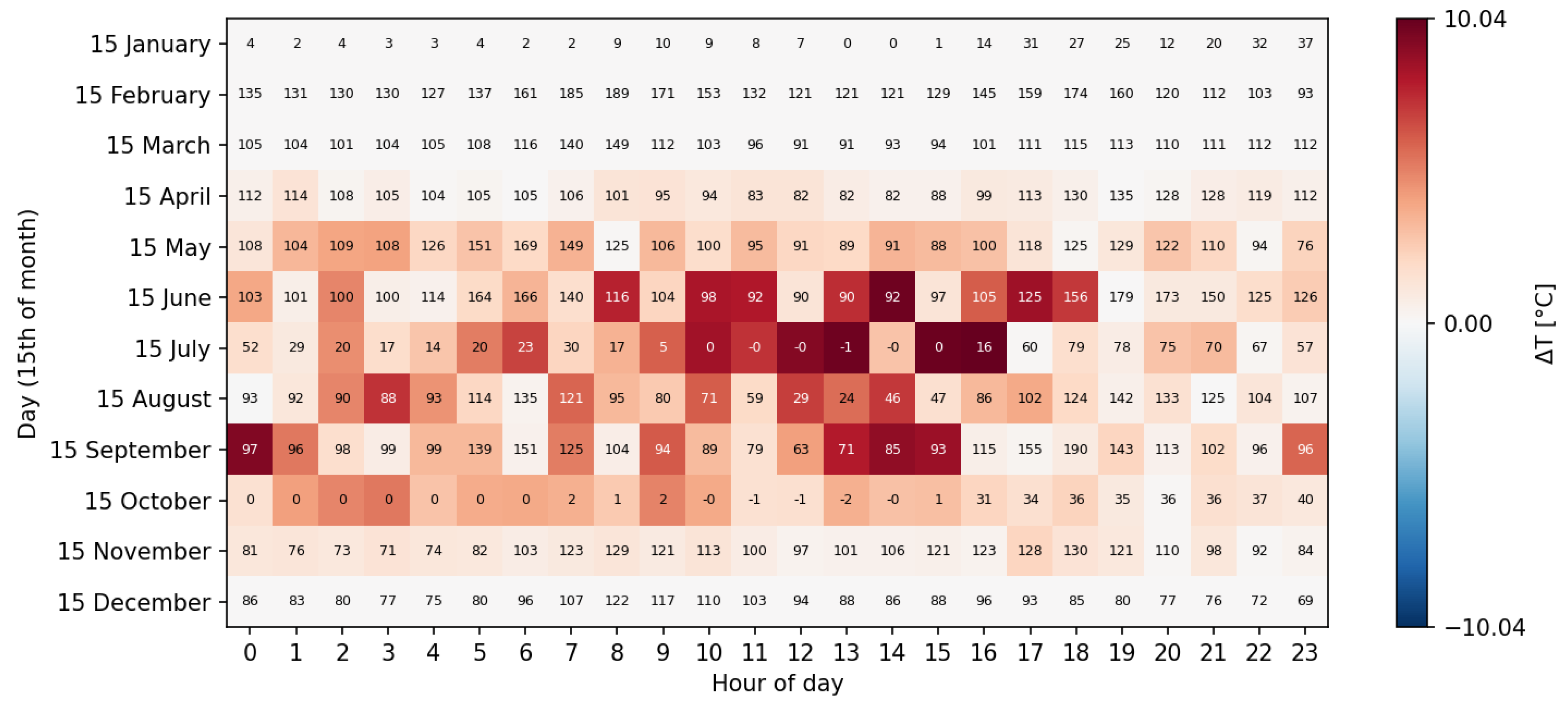
Using the developed XGBoost models for the primary cooling systems and the technical constraints of the saltwater pre-cooling unit, the proposed BO method was applied to minimize the total power consumption while meeting operational requirements. In the Business-as-Usual (BaU) scenario, the pre-cooling system lowers the saltwater temperature to 12 °C before discharge into the breeding pools. However, in the optimized model, the discharge temperature is dynamically adjusted throughout the day to minimize total electricity costs. When the temperature of the water intake from the tank falls below 7 °C, the optimized model disables the pre-cooling process to comply with the system’s safety limitations. To illustrate how the proposed model responds to seasonal variations in water temperature and electricity price, Figure 14 presents the difference between the optimized discharge temperature and the original intake temperature from the water tank for the 15th day of each month.
As shown, during the colder months of January, February, March, and December there is no difference between the intake and discharge temperatures, as ambient conditions already meet the required thresholds. In contrast, during warmer months the model reduces the discharge temperature more significantly. The values inside each block indicate the electricity price in €/MWh at that hour. As observed, the greatest reductions in water temperature occur when electricity prices are low or negative. This demonstrates the system’s flexibility to shift consumption toward low-price periods and reduce demand on the primary cooling systems, as enabled by the newly installed pre-cooling unit. Previously, we highlighted that the primary cooling units operate in a price-agnostic manner, focusing solely on maintaining the breeding pool temperature within safe limits. In contrast, the new pre-cooling unit adds responsiveness to price signals by actively cooling when electricity is cheap. This not only increases operational flexibility but also lowers the load on the primary systems, particularly in warmer months. Finally, the most significant flexibility contributions from the system occur during warm periods, when higher ambient temperatures demand more cooling effort.
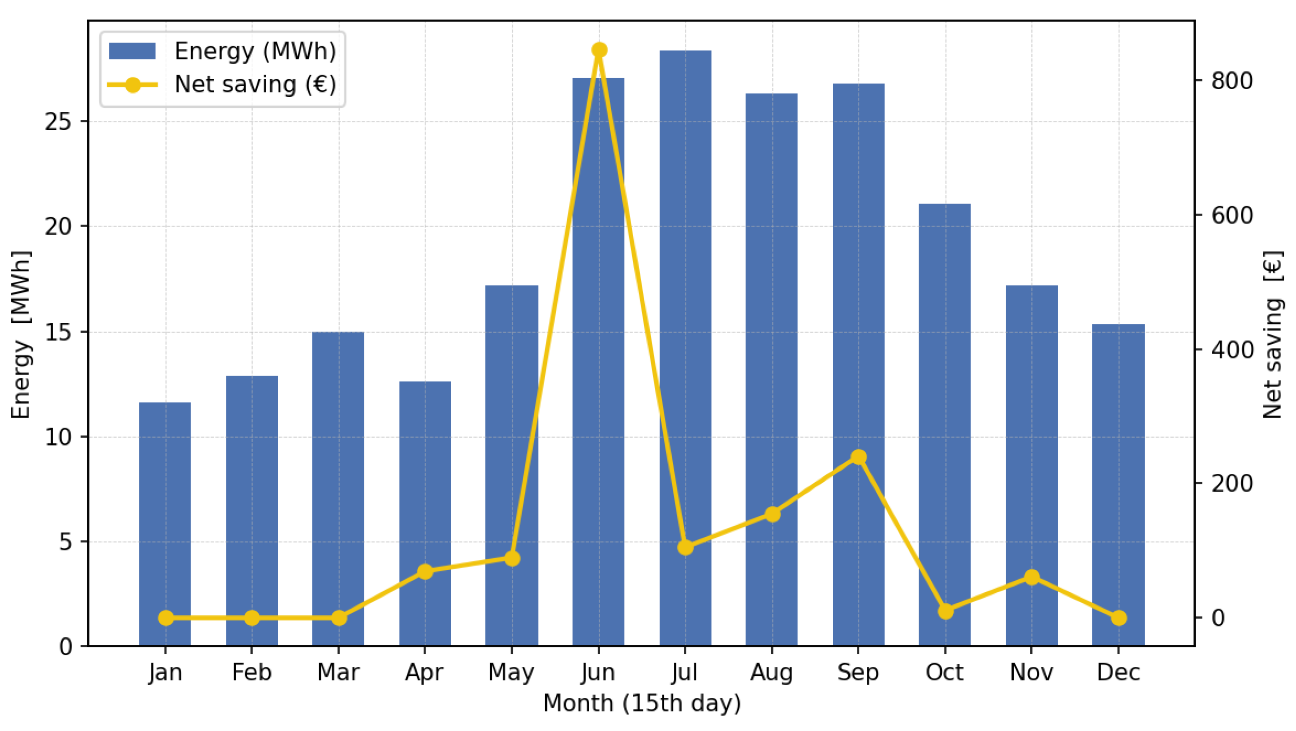
Figure 15 illustrates the total energy consumption and net savings achieved on the 15th of each month after utilization of the optimized model.
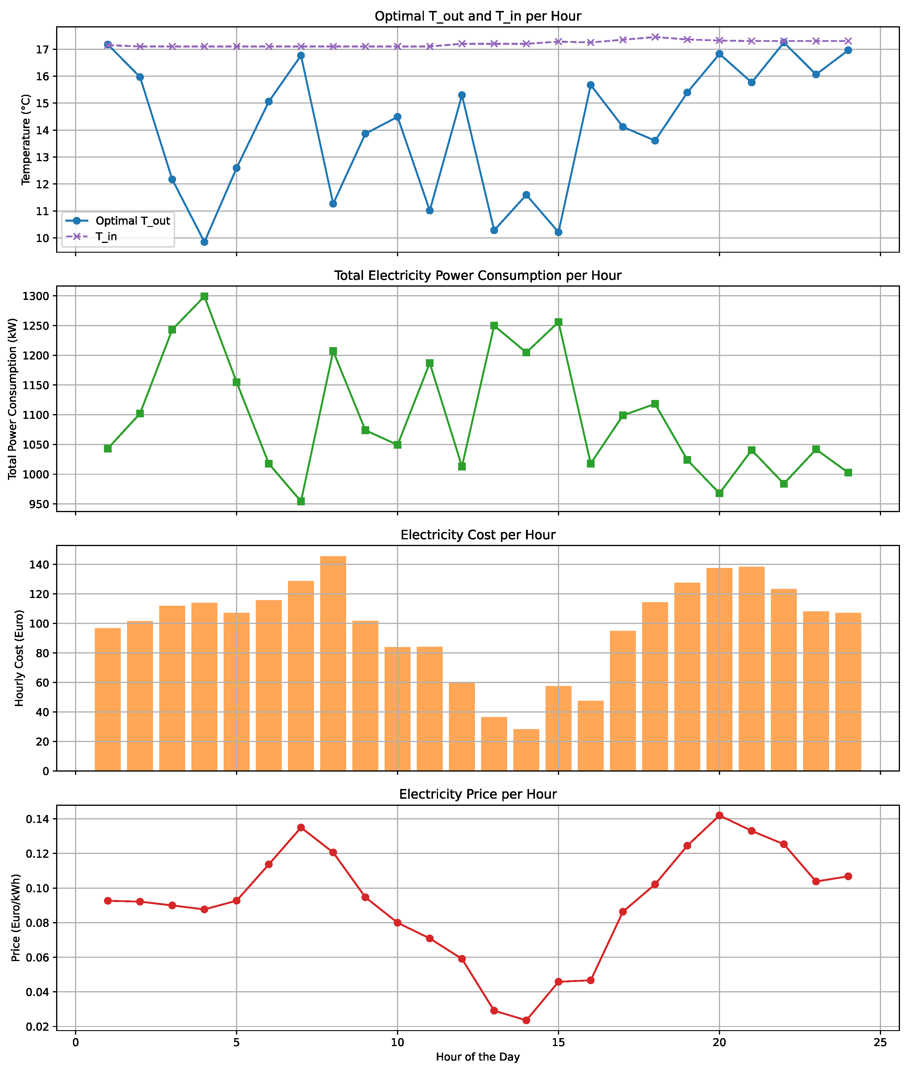
As expected, energy consumption increases during warmer months due to higher cooling demand. On the other hand, in colder months most energy use stems from internal heat sources such as fish metabolism and machinery. Net savings peak in June, driven by the combined effect of high intake water temperature and elevated electricity prices demonstrate the value of flexibility under these conditions. After examining seasonal trends, it is also useful to assess system behavior within a single day. Figure 16 presents simulation results for 15 August 2023, one of the hottest days of the year.
Figure 16 comprises four subfigures illustrating the following: (1) the optimal discharge temperature alongside the intake temperature from the water tank; (2) the total hourly power consumption of the three cooling systems; (3) the hourly electricity cost; and (4) the electricity price on 15 August 2023. The results emphasize that when electricity prices are high, the system reduces cooling intensity to lower power consumption; conversely, during mid-day, when prices decline, the model increases cooling, leading to higher power usage. Although the cost per unit of electricity is low at mid-day, the corresponding increase in power consumption highlights the model’s effectiveness in shifting operations from price-agnostic to price-responsive behavior. Ultimately, this flexible strategy yields a total electricity cost of EUR 3245.70, representing a 4.5% reduction compared to the BaU scenario. For a broader daily comparison, Table 4 presents the total electricity costs and percentage savings for both scenarios during the second week of August, a period marked by high seawater temperatures.
As shown in Table 4, the proposed method consistently achieves lower operational costs compared to the BaU scenario, particularly on days with elevated water temperatures. Notably, on the first day of the second week of August, after electricity prices reached negative levels, the model strategically increased water cooling to maximize profit. This clearly demonstrates its ability to operate in a more flexible and cost-effective manner. On other days, the model effectively adjusted the discharge temperature of the water entering the breeding pools, minimizing operational costs while maintaining the required thermal conditions. Overall, implementing the proposed model resulted in a 5.41% reduction in the total operational cost for the week despite limited access to detailed system data. This highlights the value of flexibility, especially during warmer periods. The flexibility analysis also reveals that integrating additional flexible assets within the factory could further reduce operating costs by enhancing the system’s responsiveness to electricity prices. Moreover, such flexibility provides technical benefits for grid operators. Specifically, when industrial consumers adapt their behavior in response to dynamic tariff signals, grid operators can better manage demand profiles, mitigate congestion, and improve overall grid reliability. This dual advantage not only delivers financial benefits to industries but also supports the broader objectives of grid stability and efficiency.
4. Conclusions

The main objective of this paper is to leverage the inherent flexibility of cooling systems in the aquaculture industry in order to minimize daily electricity costs. To accomplish this, the XGBoost algorithm was employed to predict the power consumption of the primary cooling systems based on a limited set of available data. The results confirmed that the proposed method can accurately capture the power consumption patterns of the systems under study. Building upon this nonlinear relationship and in combination with the technical constraints of the pre-cooling unit, the optimal discharge temperature of water into the breeding pools was determined using a Bayesian Optimization approach. The findings demonstrate that the proposed model can significantly reduce total electricity costs compared to the BaU scenario, highlighting the potential for energy and cost savings in energy-intensive industries such as aquaculture. In addition, this study underscores the effectiveness of machine learning in optimizing industrial operations even in situations with sparse data. The same black-box modeling strategy can be extended to other energy-intensive systems beyond aquaculture, including district and urban cooling networks, commercial real estate HVAC systems, and cold-storage facilities, where flexible assets such as compressors, chillers, and pumps can be co-optimized for both operational efficiency and grid-interactive services. Finally, this work outlines a clear pathway for interdisciplinary impact, as follows:
  • Utility and grid operators can integrate price-responsive industrial loads into ancillary services markets and congestion management strategies.
  • Policy-makers can design dynamic tariff schemes and demand response programs that incentivize and reward industrial flexibility.
  • Smart city planners and IoT/BMS integrators can adopt this workflow to coordinate distributed assets for enhanced efficiency and resilience.
Future research will extend this framework to support multi-site coordination as well as co-optimization with on-site renewables and energy storage systems. This will further strengthen the connection between industrial flexibility, smart grid development, energy policy, and sustainable urban infrastructure.

Author Contributions

Conceptualization, S.G., H.G., A.A.-M. and B.B.-J.; methodology, S.G. and H.G.; software, S.G.; validation, S.G. and H.G.; formal analysis, S.G. and H.G.; investigation, S.G., H.G. and A.A.-M.; writing—original draft preparation, S.G. and H.G.; writing—review and editing, S.G., H.G., A.A.-M. and B.B.-J.; visualization, S.G.; supervision, A.A.-M. and B.B.-J.; funding acquisition, B.B.-J. All authors have read and agreed to the published version of the manuscript.

Funding

This research was funded by the ELFORSK program under the Danish Energy Agency grant number ELF221-496872.

Data Availability Statement

Data available on request due to restrictions (e.g., privacy, legal or ethical reasons).

Conflicts of Interest

The authors declare no conflicts of interest.

References

  1. Jeyaraj, T.; Ponnusamy, A.; Selvaraj, D. Hybrid renewable energy systems stability analysis through future advancement technique: A review. Appl. Energy 2025, 383, 125355. [Google Scholar] [CrossRef]
  2. Wu, J.; Li, L.; Zhang, J. Maximum demand flexibility from the demand response of a big group of residential homes. Int. J. Electr. Power Energy Syst. 2023, 147, 108800. [Google Scholar] [CrossRef]
  3. Vanage, S.; Cetin, K.; McCalley, J.; Wang, Y. Grid-scale demand-side flexibility services using commercial buildings lighting loads. Energy Build. 2023, 300, 113631. [Google Scholar] [CrossRef]
  4. Penuela, J.; Ben, C.; Boldyrev, S.; Gentzbittel, L.; Ouerdane, H. The indoor agriculture industry: A promising player in demand response services. Appl. Energy 2024, 372, 123756. [Google Scholar] [CrossRef]
  5. Ranaboldo, M.; Aragüés-Peñalba, M.; Arica, E.; Bade, A.; Bullich-Massagué, E.; Burgio, A.; Caccamo, C.; Caprara, A.; Cimmino, D.; Domenech, B.; et al. A comprehensive overview of industrial demand response status in Europe. Renew. Sustain. Energy Rev. 2024, 203, 114797. [Google Scholar] [CrossRef]
  6. Golmohamadi, H.; Keypour, R.; Bak-Jensen, B.; Pillai, J.R.; Khooban, M.H. Robust Self-Scheduling of Operational Processes for Industrial Demand Response Aggregators. IEEE Trans. Ind. Electron. 2020, 67, 1387–1395. [Google Scholar] [CrossRef]
  7. Boldrini, A.; Koolen, D.; Crijns-Graus, W.; Worrell, E.; van den Broek, M. Flexibility options in a decarbonising iron and steel industry. Renew. Sustain. Energy Rev. 2024, 189, 113988. [Google Scholar] [CrossRef]
  8. Golmohamadi, H.; Asadi, A. Integration of Joint Power-Heat Flexibility of Oil Refinery Industries to Uncertain Energy Markets. Energies 2020, 13, 4874. [Google Scholar] [CrossRef]
  9. Alnahhal, Z.; Shaaban, M.F.; Hamouda, M.A.; Majozi, T.; Bardan, M.A. A Water-Energy Nexus Approach for the Co-Optimization of Electric and Water Systems. IEEE Access 2023, 11, 28762–28770. [Google Scholar] [CrossRef]
  10. Aghajanzadeh, A.; Therkelsen, P. Agricultural demand response for decarbonizing the electricity grid. J. Clean. Prod. 2019, 220, 827–835. [Google Scholar] [CrossRef]
  11. Golmohamadi, H.; Asadi, A. A multi-stage stochastic energy management of responsive irrigation pumps in dynamic electricity markets. Appl. Energy 2020, 265, 114804. [Google Scholar] [CrossRef]
  12. Han, Z.; Wang, K.; Dai, L.; Li, K.; Wang, X. Recent Application of Heat Pump Systems for Environmental Control in Livestock Facilities–A Review. Agriculture 2024, 14, 2309. [Google Scholar] [CrossRef]
  13. Crawley, J.; Moore, G.; Higginson, S.; Elwell, C.; Eyre, N. The Role of Domestic Heat Pumps in Providing Flexibility to the UK Electricity System. Energies 2024, 17, 2995. [Google Scholar] [CrossRef]
  14. Fathollahzadeh, M.H.; Tabares-Velasco, P.C. Electric demand minimization of existing district chiller plants with rigid or flexible thermal demand. Appl. Energy 2021, 289, 116664. [Google Scholar] [CrossRef]
  15. Zhu, T.; Du, Y.; Liang, J.; Rohlfs, W.; Eric Thorsen, J.; Elmegaard, B. Integration of booster heat pumps in ultra-low temperature district heating network: Prototype demonstration and refrigerant charge investigation. Energy Build. 2023, 298, 113516. [Google Scholar] [CrossRef]
  16. Shahcheraghian, A.; Madani, H.; Ilinca, A. From White to Black-Box Models: A Review of Simulation Tools for Building Energy Management and Their Application in Consulting Practices. Energies 2024, 17, 376. [Google Scholar] [CrossRef]
  17. Bahramara, S. Robust Optimization of the Flexibility-constrained Energy Management Problem for a Smart Home with Rooftop Photovoltaic and an Energy Storage. J. Energy Storage 2021, 36, 102358. [Google Scholar] [CrossRef]
  18. Stegemerten, F.; Leidolf, S.; Stoffel, P.; Müller, D. Exploring flexibility in building energy systems: Agent-based quantification and electricity tariff impacts. Energy Build. 2025, 334, 115500. [Google Scholar] [CrossRef]
  19. El Makroum, R.; Khallaayoun, A.; Lghoul, R.; Mehta, K.; Zörner, W. Home Energy Management System Based on Genetic Algorithm for Load Scheduling: A Case Study Based on Real Life Consumption Data. Energies 2023, 16, 2698. [Google Scholar] [CrossRef]
  20. Golmohamadi, H.; Guldstrand Larsen, K.; Gjøl Jensen, P.; Riaz Hasrat, I. Optimization of power-to-heat flexibility for residential buildings in response to day-ahead electricity price. Energy Build. 2021, 232, 110665. [Google Scholar] [CrossRef]
  21. Lahariya, M.; Karami, F.; Develder, C.; Crevecoeur, G. Physics-Informed LSTM Network for Flexibility Identification in Evaporative Cooling System. IEEE Trans. Ind. Inform. 2023, 19, 1484–1494. [Google Scholar] [CrossRef]
  22. Zhang, P.; Jia, Y.; Shang, Y. Research and application of XGBoost in imbalanced data. Int. J. Distrib. Sens. Netw. 2022, 18, 15501329221106935. [Google Scholar] [CrossRef]
  23. Frazier, P.I. A tutorial on Bayesian optimization. arXiv 2018, arXiv:1807.02811. [Google Scholar]
Figure 1. Typical schematic of cooling system configuration in aquaculture industry.
Applsci 15 06273 g001
Figure 2. Hourly water temperature heatmap for year 2023.
Applsci 15 06273 g002
Figure 3. Seasonal-trend decomposition of the power consumption of the ammonia cooling system for spring and summer.
Applsci 15 06273 g003
Figure 4. Seasonal-trend decomposition of the power consumption of the ammonia cooling system for autumn and winter.
Applsci 15 06273 g004
Figure 5. Seasonal-trend decomposition of the power consumption of the CO2 cooling system for spring and summer.
Applsci 15 06273 g005
Figure 6. Seasonal-trend decomposition of the power consumption of the CO2 cooling system in fall and winter.
Applsci 15 06273 g006
Figure 7. Power consumption range of ammonia cooling system per various temperature bins.
Applsci 15 06273 g007
Figure 8. Power consumption range of CO2 cooling system per various temperature bins.
Applsci 15 06273 g008
Figure 9. Comparison between the actual and predicted value across test data for the ammonia cooling system.
Applsci 15 06273 g009
Figure 10. Comparison between the actual and predicted value across test data for the CO2 cooling system.
Applsci 15 06273 g010
Figure 11. SHAP values for the ammonia cooling system.
Applsci 15 06273 g011
Figure 12. SHAP values for the CO2 cooling system.
Applsci 15 06273 g012
Figure 13. Distribution of prediction errors across various combinations of the previous hour’s power consumption and the temperature of the discharged water.
Applsci 15 06273 g013
Figure 14. Change in discharge water temperature across hours and months in the optimized model.
Applsci 15 06273 g014
Figure 15. Total energy consumption and net savings on the 15th day of each month.
Applsci 15 06273 g015
Figure 16. Simulation outputs for 15 Auguest 2023 for the considered use case.
Applsci 15 06273 g016
Table 1. Technical and economic characteristics considered in this study.
ItemValue
Primary Ammonia plantCapacity: 2.5 MW; COP: 3
Primary CO2 plantCapacity: 3 MW; COP: 2.5
Precooling CO2 plantCapacity: 2.5 MW; COP: 2.5
Threshold temperature:12 °C
Mass flow rate from tank150 m3/h
Mass flow rate discharging to pools75 m3/h
Electricity PriceDynamic for 2023 1
1 Source: www.energidataservice.dk/tso-electricity/Elspotprices, accessed on 29 May 2025.
Table 2. Evaluation of the effectiveness of the various methods in modeling the ammonia plant.
MethodMAEMSERMSER2
Proposed16.82825.9128.730.97
Random Forest17.671000.7631.630.96
Linear Regression18.191033.7732.150.96
SVR26.191306.3136.140.95
Table 3. Evaluation of the effectiveness of the various methods in modeling the CO2 plant.
MethodMAEMSERMSER2
Proposed22.291943.9944.090.91
Random Forest22.502181.3246.700.89
Linear Regression23.521991.0544.620.90
SVR30.002687.1451.830.87
Table 4. Evaluation of the effectiveness of the various methods in modeling the CO2 plant.
DayProposed Method (Euro)BAU (Euro)Saving% of Improvement
8 August 2023−187.14−168.6718.4710.95
9 August 2023270.26289.7419.4746.72
10 August 20231453.711570.16116.457.41
11 August 20232533.282631.0097.723.71
12 August 20232157.412188.2030.781.40
13 August 20231655.631767.49111.856.32
14 August 20232651.102859.40208.307.28
Disclaimer/Publisher’s Note: The statements, opinions and data contained in all publications are solely those of the individual author(s) and contributor(s) and not of MDPI and/or the editor(s). MDPI and/or the editor(s) disclaim responsibility for any injury to people or property resulting from any ideas, methods, instructions or products referred to in the content.