1. Introduction
As renewable energy sources such as wind and solar become increasingly integrated into the power system, the intermittency of the electricity supply is increasing significantly. At the same time, the shift from passive consumers to more flexible ones such as Electrical Vehicles (EVs) is adding uncertainty to electricity demand. This combination of variable supply and unpredictable demand creates challenges for power grid stability [
1]. Energy flexibility is an effective solution to balance renewable energy fluctuations and ensure a stable power system. Below, energy flexibility is discussed from three perspectives: power supply, electricity demand, and energy storage.
On the demand side, flexibility has been explored across different sectors, including residential [
2], commercial [
3], agricultural [
4], and industrial [
5]. Each sector has unique electricity demand patterns and flexibility potential, requiring expert knowledge for effective management. Among these, the industrial sector has energy-intensive processes that can provide significant flexibility to the power grid.
Industrial plants are categorized into light, medium, and heavy industries. Light and medium industries are usually connected to distribution and sub-transmission networks, while heavy industries are often connected directly to the transmission network. This means that industrial energy management systems can help to support both distribution and transmission grids.
Certain industrial processes can be adjusted based on grid requirements. For example, recent studies have shown that crushers and milling machines used in cement manufacturing can change their power consumption with short advance notice [
6]. Similarly, in metal smelting, electric furnaces can increase or decrease their power usage with mid-term notice, helping to help stabilize the grid [
7]. Many industries also have on-site power generation (self-distributed generation), which can support the grid during power shortages. A recent study has shown that oil refineries can use their Distributed Generation (DG) units to help balance power fluctuations in the grid [
8].
In recent years, the water–energy nexus has gained attention as the water industry seeks more efficient energy usage [
9]. Research has suggested [
10] that restructuring the agricultural sector could improve its ability to integrate more renewable energy sources. Another [
11] showed that operation of irrigation pumps can be optimized to provide grid flexibility during peak demand hours, especially when crop water demand coincides with high electricity consumption periods.
Recent studies have shown that heat pumps are being used more in livestock industries, e.g., poultry farms, pig farms, and ranches [
12]. These heat pumps run on electricity instead of fossil fuels, and can produce 3–5 times more heat than they use in electricity. They can also help to balance electricity demand by adjusting indoor air temperatures. Because the thermal time constant is slower than electricity, heat pumps can be turned off or down when there is not enough renewable power available on the supply side [
13].
In addition to heat pumps, cooling plants are energy-intensive industrial plants in the water–energy nexus environment that can provide significant flexibility for both the heat and electricity grids [
14]. In cold storage facilities such as those for meat and fish, cooling systems remove heat from the stored goods by consuming electricity. The waste heat that is removed can then be directly fed into the district heating network or used by booster heat pumps to improve the efficiency of district heating [
15].
Current research on energy flexibility shows that many potential sources of flexibility in different demand sectors remain underexplored. In order to unlock this flexibility without compromising comfort or safety, expert knowledge is essential. In addition to identifying flexibility potentials, the state of the art also explores various methods for optimizing energy flexibility. In this way, depending on the availability of data and the characteristics of the energy system under study, such systems can be modeled as a white-box, grey-box, or black-box system [
16]. A white-box model is used when detailed knowledge about the system’s operation and constraints is available. In such cases, the system is described using physical and mathematical equations with clearly defined constraints. These models can be solved using optimization tools such as CPLEX for linear problems [
17], while solvers such as IPOPT or KNITRO are suitable for nonlinear cases [
18]. For highly nonlinear or complex systems where conventional solvers may struggle, heuristic methods such as genetic algorithms or Particle Swarm Optimization (PSO) can be applied [
19]. When partial knowledge of the system exists and some historical or real-time data is available, a grey-box model can be developed by combining physical insights with data-driven components. In [
20], a continuous-time stochastic grey-box model was initially developed at DTU Compute and further improved at AAU Computer Science to unlock energy flexibility in buildings with multiple temperature zones. In situations where the internal characteristics of the system are largely unknown and only data are available, black-box model can be appropriate. In this approach, machine learning algorithms are used to model and optimize system behavior. Studies have shown that neural networks and Long Short-Term Memory (LSTM) models are effective in capturing and utilizing the flexibility potential of industries, especially when detailed system information is lacking [
21].
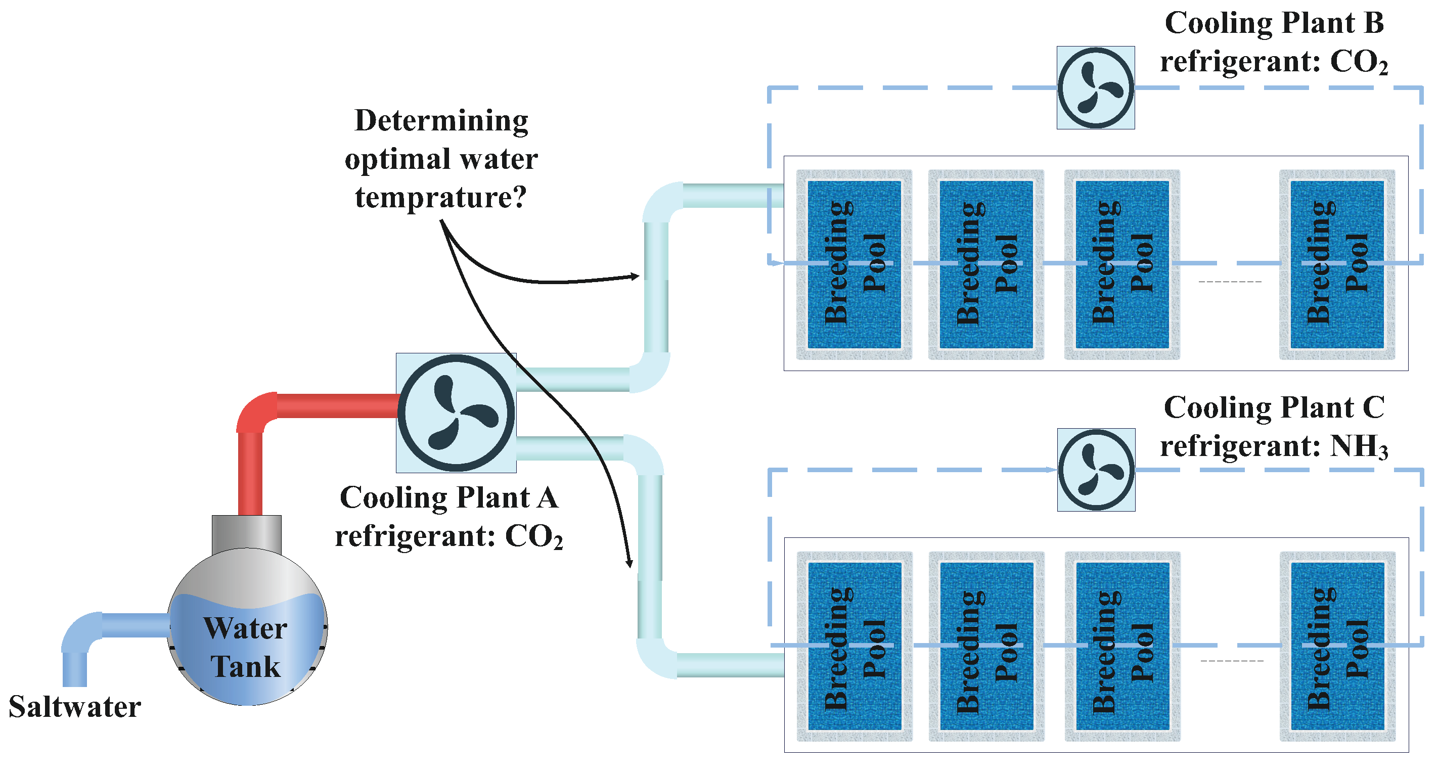
This paper explores the energy flexibility potential of salmon fish breeding pools that are supported by industrial cooling plants. These cooling plants receive brine water from the sea, which is treated and then cooled or heated to maintain the required temperature range in the breeding pools. The temperature in these pools must stay within a specific range, which can be influenced by outdoor conditions. Flexibility arises from the fact that the water temperature does not need to be kept at a single fixed value but can vary within a safe range. Based on this, an intelligent control system is developed for the cooling plant to take advantage of this thermal flexibility and respond dynamically to fluctuations in electricity prices. The study is based on a real-world case located in the Port of Hirtshals in northern Denmark. Real operational data from the plant are used to create a black-box model of the system. This model is then optimized using Extreme Gradient Boosting (XGBoost) and Bayesian Optimization to improve control strategies and unlock flexibility.
The main contributions of this study are as follows:
Developing a black-box model for the energy consumption of a cooling plant that supplies a fish breeding pool while considering flexible temperature bounds.
Demonstrating the ability to unlock power-to-heat flexibility in response to dynamic electricity prices.
Optimizing the flexibility potential of the cooling plant using XGBoost and Bayesian Optimization supported by real-world historical data from the industrial facility.
The rest of the paper is organized as follows:
Section 2 presents the methodology of the suggested approach as well as the mathematical models and formulations;
Section 3 explains the case study and simulation results; finally, the last section concludes the study.
3. Simulation Results
The effectiveness of the proposed optimization model was evaluated in a real aquaculture industry at the Port of Hirtshals in Denmark. The facility features three cooling systems. Saltwater is drawn in through a water tank that is regularly refilled by another facility. One of the newly installed cooling systems is responsible for pre-cooling of the water prior to discharge into the breeding pools. Additionally, each breeding pool is equipped with a primary cooling system that lowers the water temperature and keeps it within acceptable bounds. Technical and economic information regarding this industry can be found in
Table 1.
Figure 2 illustrates the hourly heatmap of the saltwater temperature intake from the water tank in 2023.
As expected, as summer approaches, the temperature of the water rises; closer to winter, the colder water reduces the need for operation of the cooling systems. In the industry under study, two cooling systems are responsible for reducing the water temperature, while the third system is used for pre-cooling. The power consumption of these systems was measured in different hours from the year 2023.
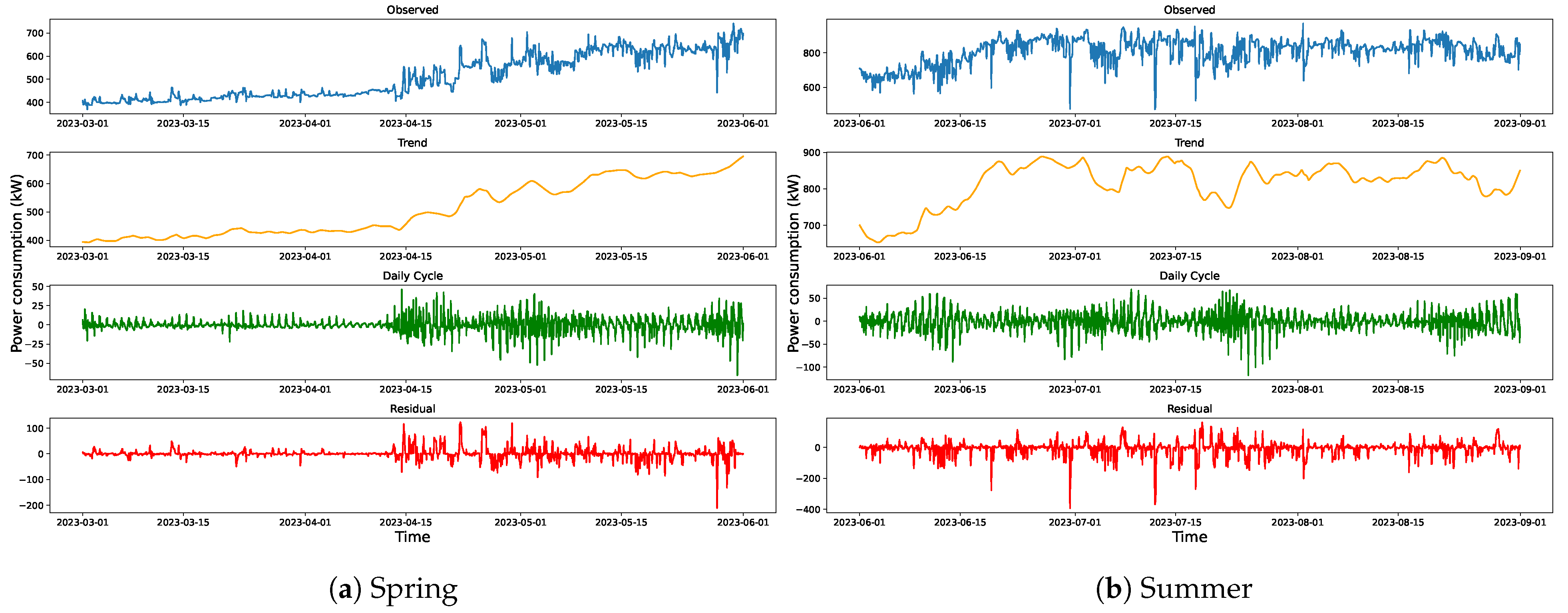
Figure 3 demonstrates the seasonal-trend decomposition of the power consumption of the ammonia cooling system using the Loess method for two seasons, namely, spring and summer.
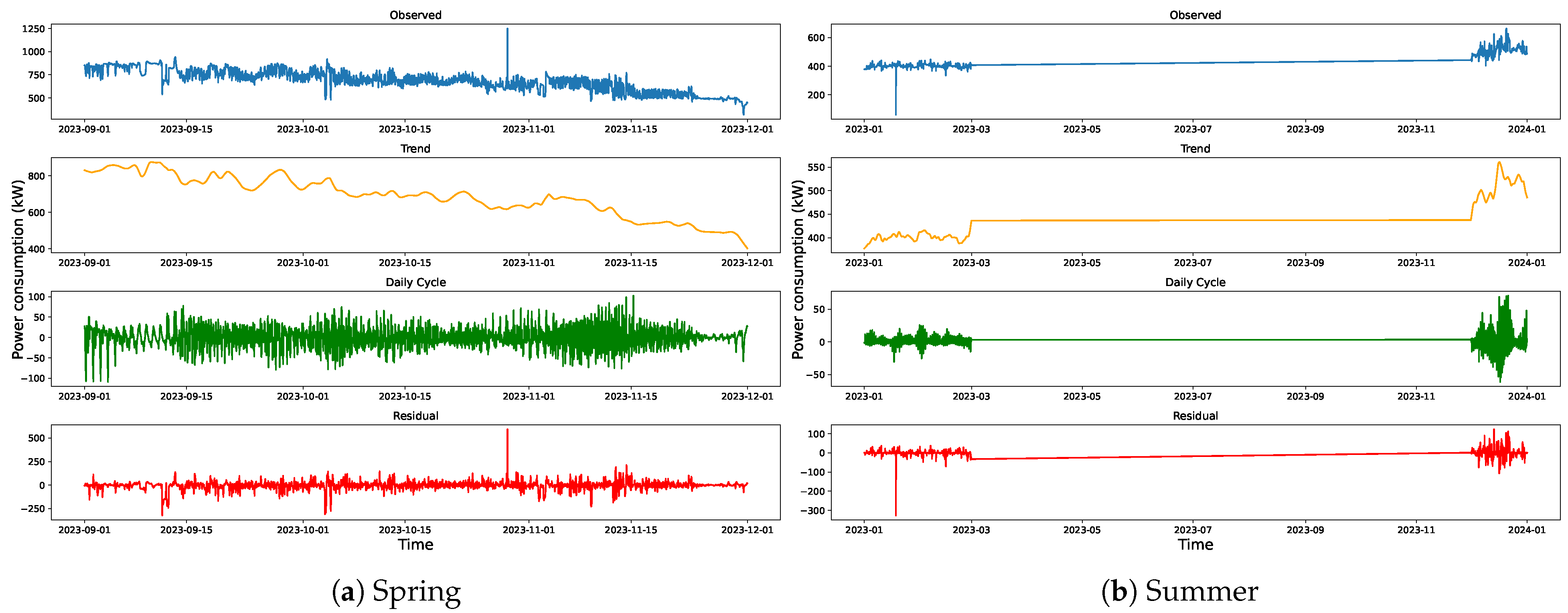
According to this technique, the observed data were decomposed into three components: trend, daily cycle, and residual. The trend component graph illustrates the long-term progression of power consumption by eliminating short-term fluctuations. As shown in the spring graph, power consumption increases as summer approaches, likely due to higher saltwater temperatures. However, fluctuations in the trend during summer can be attributed to variations in water temperature throughout the season, and the maximum power consumption reaches nearly 900 kW. The daily cycle component extracts the portion of the power consumption data that repeats every 24 h, helping to identify the hours when peaks and valleys occur. Finally, the residual component captures what remains after removing both the trend and daily cycle from the observed data, highlighting potential outliers, measurement errors, or unexpected events impacting the cooling system. It is noteworthy to mention that significant residual values during certain hours suggest that these periods warrant further investigation. A similar decomposition analysis was applied to the power consumption of this unit in autumn and winter, with the results shown in
Figure 4.
In contrast to the summer trend, the autumn trend component shows a reduction in the cooling system’s power consumption as winter approaches. Moreover, the residual values are insignificant for most hours, which improves the prediction of power consumption based on the trend and daily cycle patterns. Furthermore, when examining the decomposition results for winter, we observe that for most hours the power consumption is zero, indicating that during those periods the water temperature is below a specific threshold and the cooling system does not need to operate. After addressing the seasonal-trend decomposition for the ammonia cooling system, it should be mentioned that the decomposition residuals average 44 kW and 47 kW in summer and fall, respectively, with a Coefficient of Variation (CV) close to 6%, compared to 19 kW and 21 kW with a CV near 4% in winter and spring. The increase in residuals during the warmer seasons can be attributed to two key factors: (1) higher condensing temperatures, and (2) more frequent fish-handling activities, which result in short but intense bursts of metabolic heat. These results suggest that the residual variability is primarily driven by predictable exogenous events rather than model mis-specification.
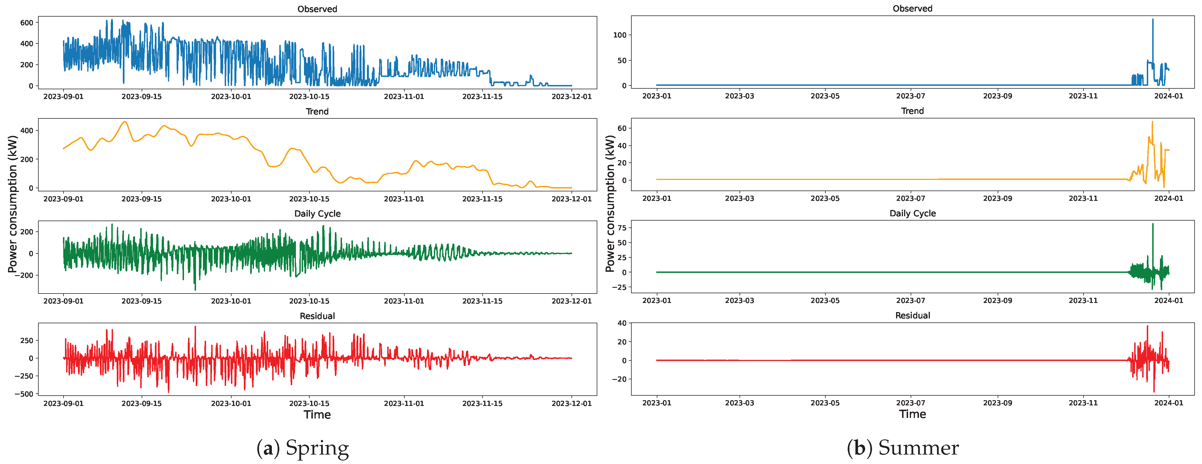
A similar analysis was performed for the CO
2 cooling system, and the decomposition of its power consumption in spring and summer are provided in
Figure 5.
The trend component for spring shows that for most hours of the season the cooling system remains in standby mode with minimal power usage, as the breeding pool’s water temperature stays below the threshold; however, in the summer greater fluctuations in water temperature lead to more variation in the trend component. Additionally, the high variability in the residual component suggests the influence of other significant factors such as fish metabolism, unexpected events, or increased machinery heat production, making the system’s prediction more challenging.
Figure 6 presents the same analysis for the following two seasons.
It is apparent from
Figure 6 that as winter approaches and water temperatures decrease, the power consumption of this unit declines, following a predictable daily cycle; however, the same challenge observed in the previous season persists. High residual values indicate the presence of other influential factors affecting the cooling system’s operation. Additionally, similar to the ammonia cooling system in winter, this cooling system operates in standby mode with minimal power consumption due to the lower saltwater temperature. For the CO
2 cascade loop, the residual standard deviation reaches 86 kW in summer and 100 kW in fall, with corresponding CVs of 35% and 52%, respectively. This elevated variability can be explained from two perspectives: first, irregular bursts of metabolic or machinery heat from warm-season activities may contribute to erratic load spikes; second, the trans-critical CO
2 compressor operates near its pressure limit during these periods, making it more sensitive to brief suction-pressure disturbances. In contrast, during winter and spring the system is largely idle and the mean power consumption drops below 10 kW, meaning that even minor startup or defrost pulses result in a CV exceeding 50%.
As reviewed in the decomposition analysis, the most prominent factor in the power consumption of the cooling systems associated with breeding pools is the temperature of the water discharged to these pools. In this regard,
Figure 7 categorizes the power consumption of the ammonia cooling systems based on water temperature bins.
As expected, higher water temperatures correlate with increased power consumption in the cooling system. However, the presence of outliers in certain bins indicates deviations from the expected pattern, suggesting unusual events that warrant further investigation of the recorded data. A similar analysis was conducted for the other cooling system.
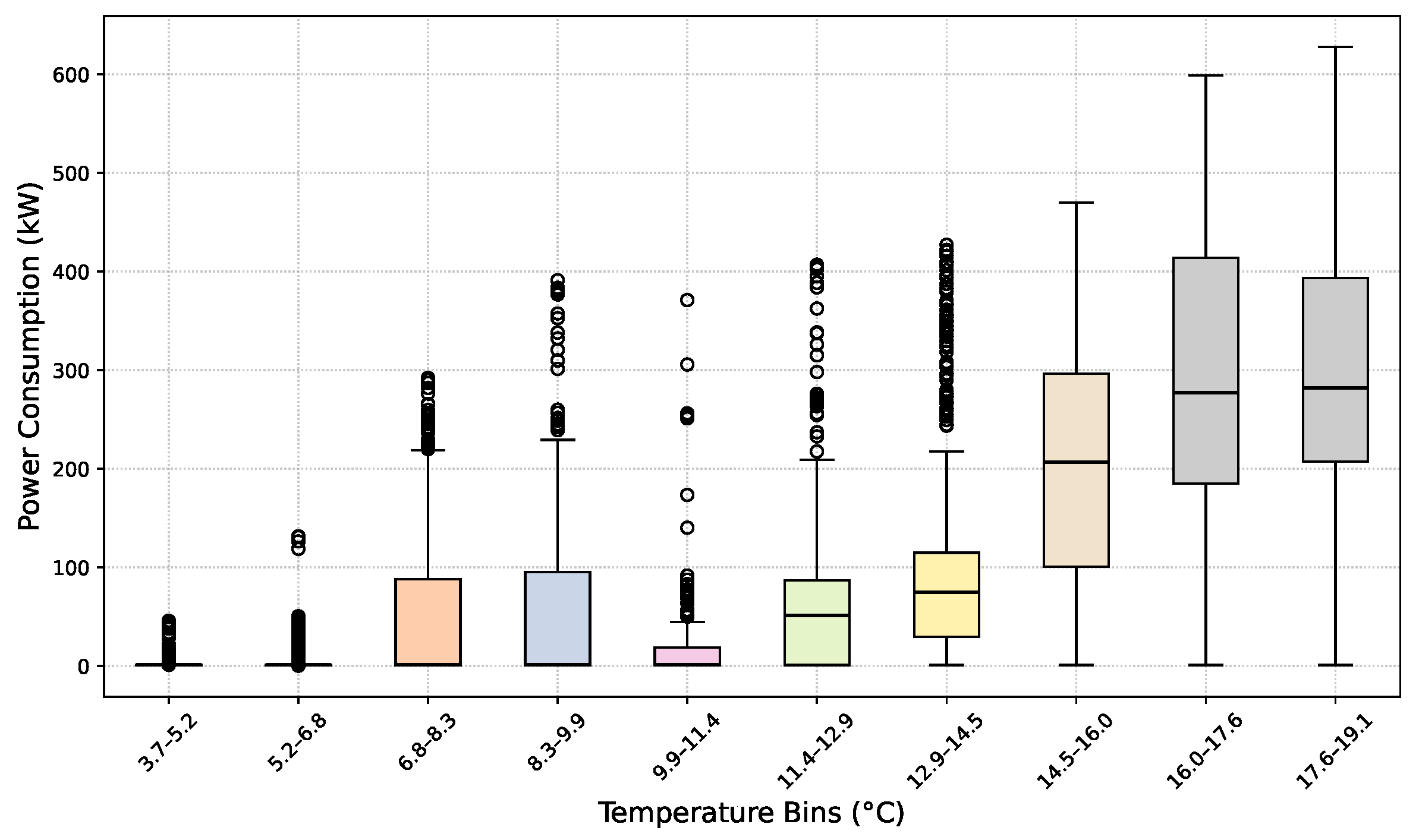
Figure 8 shows the power consumption distribution across different temperature bins for the CO
2 cooling system.
Again, higher temperatures lead to increased power consumption; however, the significant variability at higher temperatures and the presence of outliers at lower temperatures suggest additional hidden factors influencing the unit’s operation. This complexity makes predicting power consumption more challenging. According to our deep review of the power consumption of the two primary cooling systems, it can be concluded that due to higher values for the residual components in certain hours, finding the accurate pattern for these systems is demanding and requires more information. However, leveraging the strengths of XGBoost can help to find the nonlinear relation between the input features and the power consumption of the cooling systems, covering the aforementioned challenge. First, Grid Search Optimization is used to find the optimal hyperparameters of this technique, according to which the best fit can be estimated.
Figure 9 shows the actual and optimized XGBoost predicted power consumption of the ammonia cooling system for the test data.
The subfigures demonstrate that the optimized XGBoost model accurately predicts the cooling system’s power consumption by leveraging the three selected feature types, effectively capturing its consumption patterns. In this regard,
Table 2 compares the model’s performance against existing methods using various evaluation metrics.
As shown in
Table 2, the proposed XGBoost model outperforms existing techniques across three error evaluation metrics. Additionally, its high
value indicates strong accuracy despite variability in observed consumption data. A similar analysis was conducted for the other cooling system, and
Figure 10 compares the predicted power consumption to the actual test data.
Despite the high variability in power consumption and the presence of outliers, the proposed model successfully captures the unit’s consumption pattern.
Table 3 presents the model’s performance evaluation using various error criteria.
Despite high residual variability,
Table 3 illustrates that the proposed model surpasses existing solutions in predicting the cooling system’s power consumption. Furthermore, the high
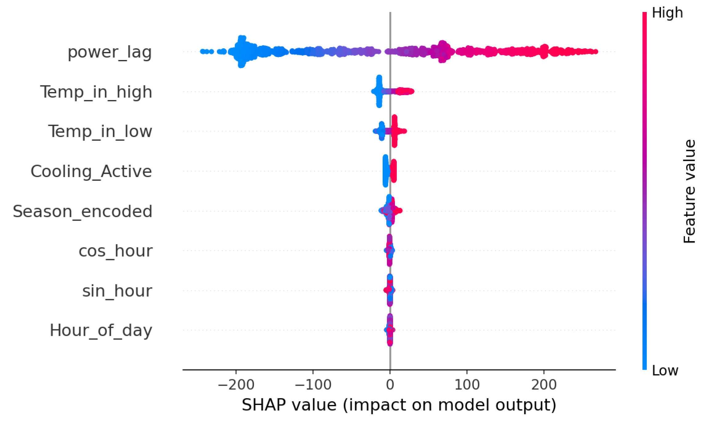
value confirms the model’s accuracy across a wide range of data variations. To assess the explainability of the developed XGBoost model, SHAP values for the ammonia cooling system were calculated using the test data. These values visually summarize the feature importance across predictions, and are presented in
Figure 11.
As shown in
Figure 11, the previous hour’s power consumption emerges as the most influential feature. If the cooling system consumed a large amount of power in the prior hour, the model assumes inertia and predicts similarly high consumption for the current hour. In addition, the temperature of the water discharged into the breeding pool is another key driver; each additional degree above 12 °C typically increases power consumption by several kilowatts. The tight and mostly positive SHAP distribution supports the intuitive linear relationship between thermal load and compressor effort. Interestingly, when the water temperature is significantly below the threshold value (represented by Temp_in_low in
Figure 11), it pulls the power prediction downward, suggesting reduced energy demand. However, temperatures close to the threshold do not significantly affect the forecast on their own. A binary indicator capturing the system’s operational status is also included. When the system is active (indicator = 1, shown in red), the SHAP values are generally positive, whereas inactive states (indicator = 0, shown in blue) correspond to near-zero or slightly negative values. However, this flag is less impactful than the actual temperature deviation. Seasonal effects have a moderate influence. Higher numeric values corresponding to summer and autumn yield slightly positive SHAP values, indicating a small expected increase in power consumption during warmer months after accounting for real-time temperature. Finally, circadian patterns contribute subtle refinements to the forecast, typically in the range of ±10 kW. Their centered distribution implies that these features help to fine-tune predictions rather than drive them. Indeed, the SHAP analysis suggests that this unit’s operation is primarily reactive, focused on maintaining water temperature rather than on strategically aligned with dynamic electricity pricing. This behavior highlights the system’s role in thermal regulation rather than economic optimization. A similar analysis is provided for the other main cooling system with CO
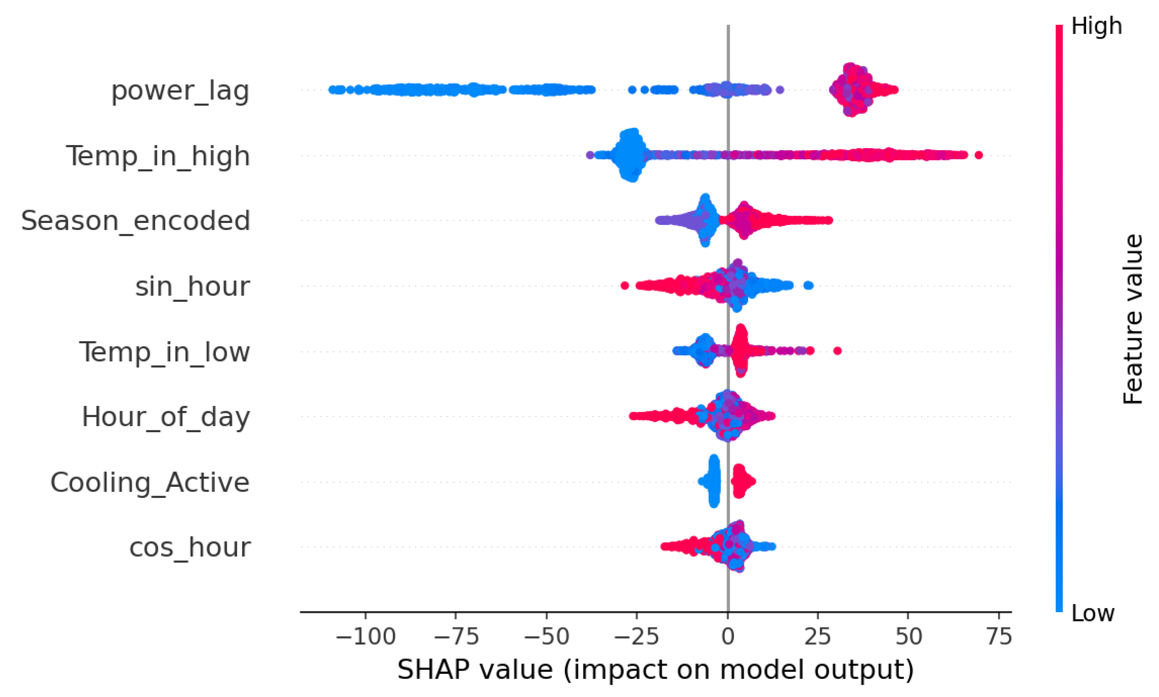
2 refrigerant, which can be found in
Figure 12.
Similar to the previous cooling system, the previous hour’s power consumption plays a dominant role in predicting the current hour’s usage. This single feature effectively summarizes various hidden factors such as heat load, set-points, defrost cycles, door openings, and brief weather anomalies that were active during the previous hour. Because thermal energy scatters slowly, a high load in the previous hour remains the strongest predictor of current consumption. As a result, the model relies on this input more heavily than any other. From an operational standpoint, this implies that smoothing spikes or pre-cooling during low-price periods not only delivers immediate savings but also sets the system into a lower operational state, potentially reducing the next hour’s demand by tens of kilowatts. As expected, each additional degree above 12 °C contributes significantly to power consumption, increasing demand by tens of kilowatts. Unlike the earlier system, this unit exhibits higher power consumption (approximately 20 kW more) even after controlling for the actual water temperature during summer and autumn hours. This pattern is likely influenced by additional seasonal factors such as humidity, occupancy levels, or adjusted set-points. Finally, the daily rhythm contributes a moderate influence on consumption patterns, while the binary variable indicating whether the system is active has the least impact among all features.
As seen, the two most influential factors in predicting the power consumption of the cooling systems are the previous hour’s power consumption and the temperature of the water discharged into the breeding pools. Therefore, it is essential to examine the conditions under which the maximum prediction error occurs across different ranges of these two variables. The error is defined as the difference between the predicted and actual values (
).
Figure 13 illustrates the distribution of prediction errors across various combinations of these two key factors for each cooling system.
Upon closer inspection of the sub-figures, it is evident that the prediction errors in both models generally remain within an acceptable range across most combinations of input variables. However, the largest errors occur at the extreme points. In the sub-figure related to the ammonia cooling system, these extremes correspond to situations where the the previous hour’s power consumption is particularly high. Similarly, the next sub-figure related to the CO2 cooling system shows that the highest errors arise when there is very high power consumption in the previous hour, especially when accompanied by elevated water temperatures.
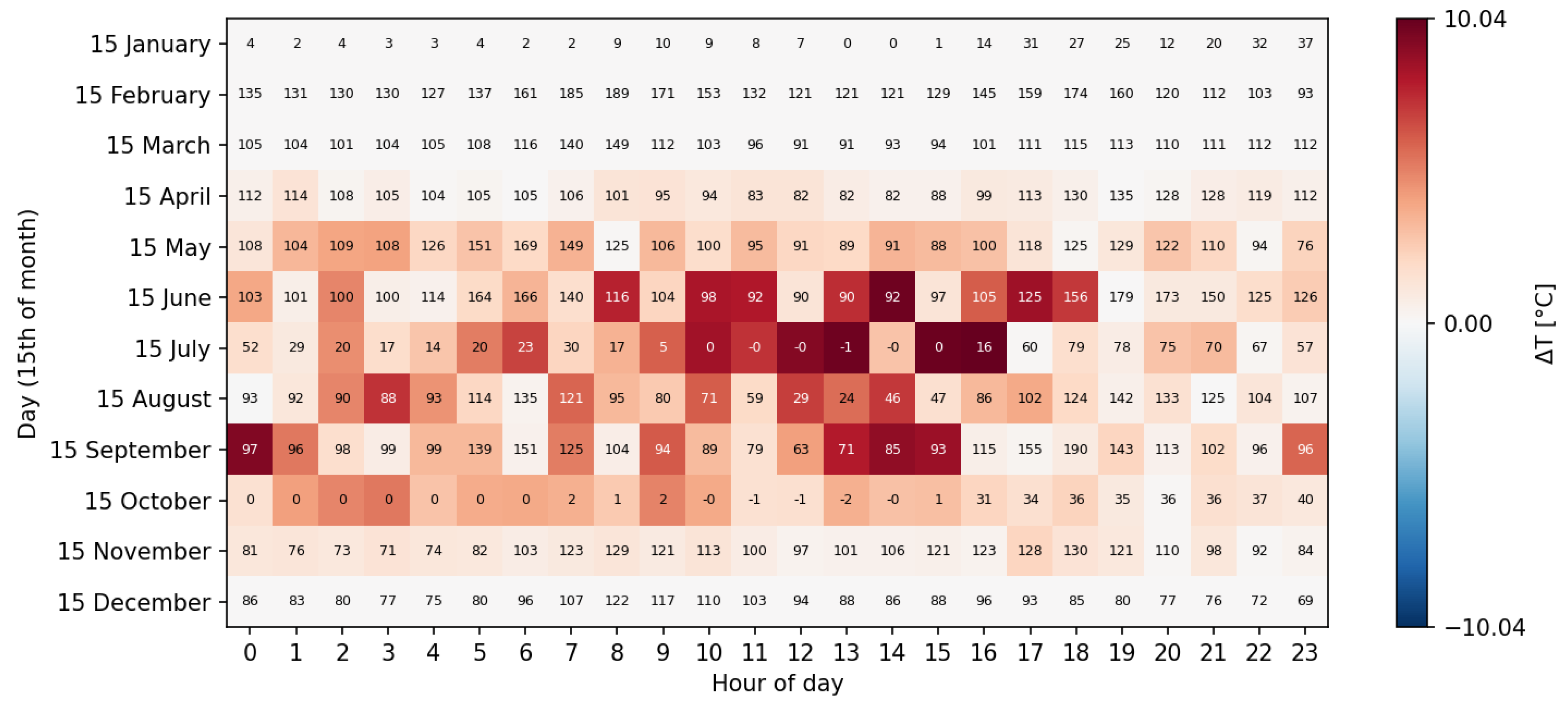
Using the developed XGBoost models for the primary cooling systems and the technical constraints of the saltwater pre-cooling unit, the proposed BO method was applied to minimize the total power consumption while meeting operational requirements. In the Business-as-Usual (BaU) scenario, the pre-cooling system lowers the saltwater temperature to 12 °C before discharge into the breeding pools. However, in the optimized model, the discharge temperature is dynamically adjusted throughout the day to minimize total electricity costs. When the temperature of the water intake from the tank falls below 7 °C, the optimized model disables the pre-cooling process to comply with the system’s safety limitations. To illustrate how the proposed model responds to seasonal variations in water temperature and electricity price,
Figure 14 presents the difference between the optimized discharge temperature and the original intake temperature from the water tank for the 15th day of each month.
As shown, during the colder months of January, February, March, and December there is no difference between the intake and discharge temperatures, as ambient conditions already meet the required thresholds. In contrast, during warmer months the model reduces the discharge temperature more significantly. The values inside each block indicate the electricity price in €/MWh at that hour. As observed, the greatest reductions in water temperature occur when electricity prices are low or negative. This demonstrates the system’s flexibility to shift consumption toward low-price periods and reduce demand on the primary cooling systems, as enabled by the newly installed pre-cooling unit. Previously, we highlighted that the primary cooling units operate in a price-agnostic manner, focusing solely on maintaining the breeding pool temperature within safe limits. In contrast, the new pre-cooling unit adds responsiveness to price signals by actively cooling when electricity is cheap. This not only increases operational flexibility but also lowers the load on the primary systems, particularly in warmer months. Finally, the most significant flexibility contributions from the system occur during warm periods, when higher ambient temperatures demand more cooling effort.
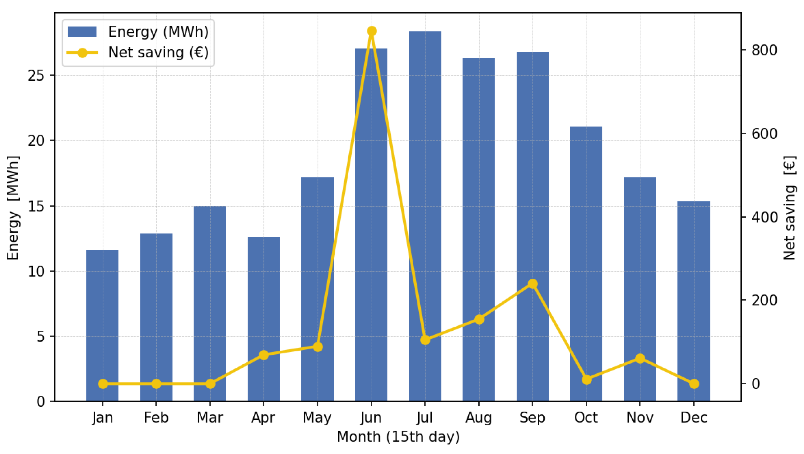
Figure 15 illustrates the total energy consumption and net savings achieved on the 15th of each month after utilization of the optimized model.
As expected, energy consumption increases during warmer months due to higher cooling demand. On the other hand, in colder months most energy use stems from internal heat sources such as fish metabolism and machinery. Net savings peak in June, driven by the combined effect of high intake water temperature and elevated electricity prices demonstrate the value of flexibility under these conditions. After examining seasonal trends, it is also useful to assess system behavior within a single day.
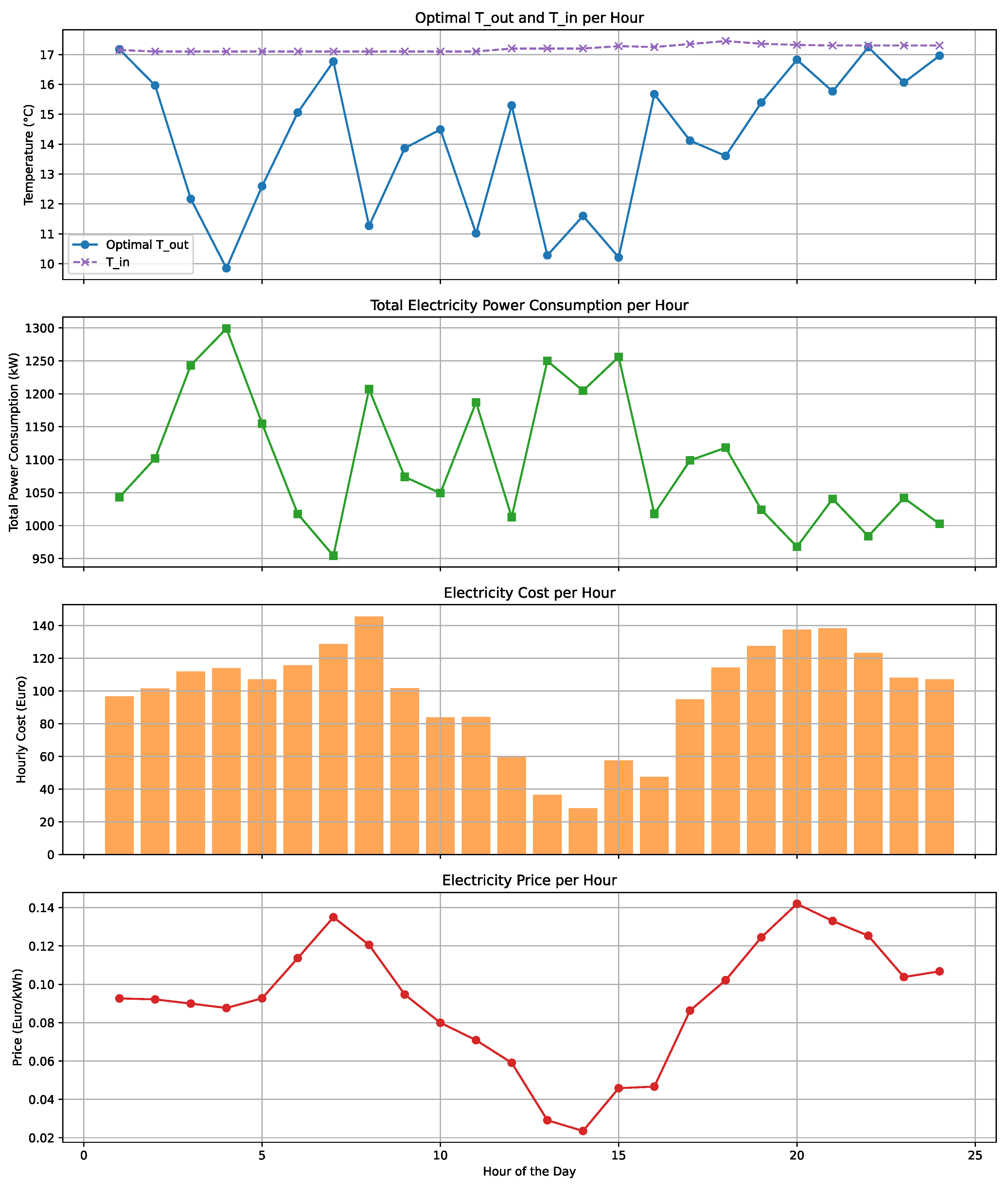
Figure 16 presents simulation results for 15 August 2023, one of the hottest days of the year.
Figure 16 comprises four subfigures illustrating the following: (1) the optimal discharge temperature alongside the intake temperature from the water tank; (2) the total hourly power consumption of the three cooling systems; (3) the hourly electricity cost; and (4) the electricity price on 15 August 2023. The results emphasize that when electricity prices are high, the system reduces cooling intensity to lower power consumption; conversely, during mid-day, when prices decline, the model increases cooling, leading to higher power usage. Although the cost per unit of electricity is low at mid-day, the corresponding increase in power consumption highlights the model’s effectiveness in shifting operations from price-agnostic to price-responsive behavior. Ultimately, this flexible strategy yields a total electricity cost of EUR 3245.70, representing a 4.5% reduction compared to the BaU scenario. For a broader daily comparison,
Table 4 presents the total electricity costs and percentage savings for both scenarios during the second week of August, a period marked by high seawater temperatures.
As shown in
Table 4, the proposed method consistently achieves lower operational costs compared to the BaU scenario, particularly on days with elevated water temperatures. Notably, on the first day of the second week of August, after electricity prices reached negative levels, the model strategically increased water cooling to maximize profit. This clearly demonstrates its ability to operate in a more flexible and cost-effective manner. On other days, the model effectively adjusted the discharge temperature of the water entering the breeding pools, minimizing operational costs while maintaining the required thermal conditions. Overall, implementing the proposed model resulted in a 5.41% reduction in the total operational cost for the week despite limited access to detailed system data. This highlights the value of flexibility, especially during warmer periods.
The flexibility analysis also reveals that integrating additional flexible assets within the factory could further reduce operating costs by enhancing the system’s responsiveness to electricity prices. Moreover, such flexibility provides technical benefits for grid operators. Specifically, when industrial consumers adapt their behavior in response to dynamic tariff signals, grid operators can better manage demand profiles, mitigate congestion, and improve overall grid reliability. This dual advantage not only delivers financial benefits to industries but also supports the broader objectives of grid stability and efficiency.


