Petrophysics Parameter Inversion and Its Application Based on the Transient Electromagnetic Method

Abstract

The transient electromagnetic (TEM) method is a widely used geophysical technique for detecting subsurface electrical structures. However, its inversion results are typically limited to resistivity parameters, making it challenging to directly infer key petrophysical properties, such as water saturation and porosity. This study proposes a petrophysics parameter inversion approach based on TEM data. By constructing multiple geoelectric models with varying porosities and water saturation values for numerical simulations, the results demonstrated that both the forward and inversion responses of the TEM field maintained errors within 5%. The inversion procedure begins with the reconstruction of the subsurface resistivity distribution, which reliably reflects the true geoelectric model. Based on the inverted resistivity, the water saturation and porosity parameters are subsequently estimated. The inversion results closely match the overall trend of the actual model and exhibit a clear response at the target layer. Finally, the proposed method is applied to a field test at the Tongxin Coal Mine. By integrating subsurface electrical responses with geological data, the spatial distributions of water saturation and porosity within the coal-bearing strata were delineated. This provides a scientific basis for the detailed characterization of the physical properties of coal and surrounding rock, as well as for understanding the development of pores and fractures in underground strata.

1. Introduction

The transient electromagnetic (TEM) method is a high-efficiency geophysical technique with deep detection capabilities that is widely applied in mineral exploration and engineering surveys [1,2]. However, conventional TEM inversion outputs resistivity distributions, which is a physical property lacking direct geological interpretability. Translating resistivity models into actionable petrophysical parameters (e.g., porosity and water saturation) remains a critical challenge for resource evaluation and hazard assessment, particularly in complex hydrogeological contexts.

Previous studies have established that the electrical conductivity of surrounding rock masses is closely related to petrophysical parameters, such as water saturation, porosity, and permeability, all of which significantly affect bulk resistivity [3,4,5]. Based on Archie’s law, Sun et al. showed that both water saturation and the formation factor influence the saturation index, with experimental results confirming the importance of formation water resistivity [6]. Nakamura et al. further quantified the relationship between resistivity and porosity, applying it to primary rock formations [7,8]. Coli et al. found strong correlations among permeability, porosity, and resistivity, which were used to infer tunnel rock properties [9]. To account for variations in water connectivity, Montaron introduced the water connectivity index (WCI), which has been successfully applied across resistivity models [10]. Yang et al. proposed a stochastic joint inversion approach for shales, revealing statistical links among petrophysical parameters [11]. Jin et al. developed an equivalent resistivity model using parallel circuit theory to relate resistivity and hydrate saturation [12]. These studies collectively highlight the critical role of petrophysical controls on resistivity and support the development of such predictive models. With the growing application of transient electromagnetic (TEM) methods in hydrogeological investigations, quantifying the coupling between EM responses and formation parameters has become increasingly vital [13,14,15]. Kafri et al. estimated aquifer porosity using TDEM-derived resistivity, improving upon Archie-based methods [16]. Choi et al. linked resistivity with Q-system classifications to assess rock mass quality [17]. Chen et al. used TEM data to quantify aquifer water content using a generalized volume model [18]. Other efforts focused on inversion methods: Killingbeck et al. proposed a Bayesian approach with depth constraints [19,20]; Cheng et al. integrated Archie’s law and deep learning to predict water-rich zones [21]. Rajab et al. and Faghih et al. applied advanced inversion strategies to map seawater intrusion and subsurface porosity [22,23]. Additional studies have explored the lithological and hydrogeological influences on resistivity in mining and karst environments [24,25,26]. Recent advances in stochastic and constrained inversion methods (e.g., BEL1D and LCI) have further improved the accuracy of resistivity-based characterization, reinforcing the potential of TEM in resolving petrophysical and hydrological conditions [27,28,29,30].

Based on the above research and analysis, inverting subsurface petrophysical parameters from transient electromagnetic (TEM) data has significant theoretical value. In this study, rock physical parameters such as porosity and water saturation were further estimated using the resistivity model obtained from TEM inversion. Multiple sets of geoelectric models with varying physical parameters were constructed for numerical simulations to verify the reliability of the proposed method. This approach provides a novel pathway for electromagnetic data inversion and facilitates the interpretation of geological data. Finally, a field TEM survey was conducted, and the spatial distribution trends of subsurface porosity and water saturation were delineated by integrating the data with geological data.

2. Theory

2.1. Forward Modeling

The transient electromagnetic (TEM) method is a time-domain electromagnetic exploration technique that uses an ungrounded loop source to transmit a step current, thereby generating a primary magnetic field in the surrounding space. This primary magnetic field induces eddy currents in subsurface geological formations, resulting in a time-varying secondary magnetic field. The secondary field is detected using a receiving coil. The temporal attenuation characteristics of the secondary field are primarily governed by the conductivity, volume, and burial depth of the anomalous body, as well as the waveform and frequency of the transmitted current. By analyzing the spatial variation of the secondary field recorded by the receiving coil, it is possible to infer the spatial distribution of subsurface anomalies. The working principle of the TEM method is illustrated in Figure 1 [31].

According to Maxwell’s equations, the propagation of electromagnetic fields in conductive media can be described by diffusion equations. Assuming a time-harmonic field e^−iωt, Maxwell’s equations can be simplified as follows [32]:

$$\nabla \times E=i\omega \mu H$$

(1)

$$\nabla \times H=\sigma E+J_s$$

(2)

where J_s is the emission current density. For an axisymmetric loop source, the field quantity depends only on the radial distance r and vertical direction z. In the cylindrical coordinate system, the vertical component Hz of the magnetic field satisfies the following scalar wave equation:

$$\left({\nabla }^2+k^2\right)H_z=0$$

(3)

where k² = iωμσ. By separation of variables, the solution can be expressed as an integral of the wave number λ:

$$H_z(r,\omega )={{\displaystyle \int }}_0^{\infty }{\tilde{H}}_z(\lambda ,\omega )J_0(\lambda r)\lambda d\lambda$$

(4)

where J₀ is the zero-order Bessel function and is the field response in the wavenumber domain.

For layered media, the reflection coefficient r_TE of the transverse electric (TE) mode is calculated using a recursive formula. The wave impedance Z_k of the kth layer is expressed as

$$Z_k={\displaystyle \frac{i\omega {\mu }_k}{{\gamma }_k}},\hspace{1em}{\gamma }_k=\sqrt{{\lambda }^2+i\omega {\mu }_k{\sigma }_k}$$

(5)

The interface reflection coefficient r_k is expressed as follows:

$$r_k={\displaystyle \frac{Z_k-Z_{k+1}}{Z_k+Z_{k+1}}}$$

(6)

The total reflection coefficient $r_{TE}^{(k)}$ is obtained through the following recursive relationship:

$$r_{TE}^{(k)}={\displaystyle \frac{r_k+r_{TE}^{(k+1)}{e}^{-2{\gamma }_k{h}_k}}{1+r_k{r}_{TE}^{(k+1)}{e}^{-2{\gamma }_k{h}_k}}}$$

(7)

where h_k is the thickness of the kth layer.

The field response ${\tilde{H}}_z(\lambda ,\omega )$ in the wavenumber domain is related to the reflection coefficient r_TE, and the spatial domain expression of the vertical magnetic field component can be obtained as:

$$H_z(r,\omega )={{\displaystyle \int }}_0^{\infty }{\displaystyle \frac{r_{TE}(\lambda ,\omega )}{i\omega \mu }}{J}_0(\lambda r)\lambda d\lambda$$

(8)

The frequency domain response is converted into the time domain perpendicular magnetic field component by a cosine transform:

$$B_z(t)={\displaystyle \frac{{\mu }_0}{2\pi }}{{\displaystyle \int }}_0^{\infty }\mathrm{Re}\left[{{\displaystyle \int }}_0^{\infty }\lambda J_0(\lambda r){\displaystyle \frac{r_{TE}(\lambda ,\omega )}{i\omega }}d\lambda \right]\cos (\omega t)d\omega$$

(9)

2.2. Inversion Algorithm

When performing a one-dimensional inversion of the loop source transient electromagnetic method, not only the fitting error between the observed data and the model data needs to be minimized, but also the roughness of the inversion model needs to be minimized. The objective function of the inversion is [33]:

$$\Phi (m)={\Phi }_d(m)+\beta {\Phi }_m(m)$$

(10)

Here, Φ_d represents the data misfit term, which quantifies the discrepancy between the predicted and observed data; Φ_m denotes the model regularization term, which imposes constraints on the model complexity; and β is the regularization parameter that balances the trade-off between data fitting and model smoothness.

The objective of inversion is to reconstruct the spatial distribution of subsurface physical parameters (e.g., resistivity, saturation, and porosity) and iteratively update the model during the inversion process so that its predicted response increasingly aligns with the observed data. The data misfit or data fitting error quantifies the discrepancy between the surface response generated by the model and the actual measured data. It is defined as:

$${\Phi }_d\left(m\right)={\displaystyle \frac{1}{2}}{‖W_d\left(F\left[m\right]-d_{obs}\right)‖}_2^2$$

(11)

where F[m] denotes the predicted data obtained through forward modeling; d_obs represents the observed data; W_d is a diagonal weighting matrix, where W_dii = 1/ε_i, and ε_i is the standard deviation of the observation error associated with the ith data point.

Since the number of field measurements is significantly smaller than the number of unknowns in the inversion model, directly minimizing the data misfit may lead to non-unique solutions. To obtain a more geologically reasonable model and reduce the ambiguity of the inversion results, this study employs the Gauss–Newton iterative optimization algorithm. The objective function, which incorporates an L₂ regularization term, is expressed as follows:

$$\Phi \left(m\right)={\displaystyle \frac{1}{2}}{‖W_d\left(F\left[m\right]-d_{obs}\right)‖}_2^2+{\displaystyle \frac{1}{2}}\beta {‖W_m\left(m-m_{ref}\right)‖}_2^2$$

(12)

Approximately solve a linear system via the conjugate gradient method as follows:

$$\left(J_k^{\top }{W}_d^{\top }{W}_d{J}_k+\beta W_m^{\top }{W}_m\right)\mathsf{\Delta }m=-J_k^{\top }{W}_d^{\top }{W}_d{r}_k-\beta W_m^{\top }{W}_m(m_k-m_{\mathrm{ref}})$$

(13)

where J_k is the Jacobian matrix, and r_k is the residual vector.

The subsurface resistivity distribution was obtained using the forward modeling and inversion techniques described above. To facilitate geological interpretation, the inversion results were further transformed from resistivity into porosity and water saturation by applying the constitutive relationships between resistivity and the rock’s physical properties. This approach enables the inversion of formation porosity and water saturation directly from the transient electromagnetic data.

To enable the inversion of rock physical parameters, it is first necessary to establish a model that relates geophysical parameters to petrophysical properties. In this study, the relationship between resistivity, porosity, and water saturation is described using Archie’s equation as follows:

$$\rho ={\rho }_w{\varphi }^{-m}{S}_w^{-n}$$

(14)

where ρ is the resistivity of the rock formation, ρ_w is the resistivity of the pore water, ϕ is the porosity, and S_w is the water saturation. The parameter m is the cementation exponent, which typically ranges from 1.3 to 3.0, and n is the saturation exponent, which is commonly taken as 2 [34].

The relationship between resistivity, porosity, and water saturation is

$$S_w={\left({\displaystyle \frac{{\rho }_w}{\rho {\varphi }^{-m}}}\right)}^{1/n},\varphi ={\left({\displaystyle \frac{{\rho }_w}{\rho S_w^{-n}}}\right)}^{1/m}$$

(15)

Inversion is performed using the nonlinear least squares method. To prevent overfitting and enhance the uniqueness and stability of the solution, a regularization term is incorporated into the objective function. The objective function for inverting the water saturation and porosity is defined as follows:

$$\Phi (m)={\displaystyle \frac{1}{2}}\parallel W_d(F(m)-d_{\mathrm{obs}}){\parallel }_2^2+{\displaystyle \frac{1}{2}}\beta \left({\lambda }_{\varphi }\parallel \varphi -{\varphi }_{\mathrm{ref}}{\parallel }_2^2+{\lambda }_{S_w}\parallel S_w-S_{w,\mathrm{ref}}{\parallel }_2^2\right)$$

(16)

where ϕ_ref and S_w,ref are the prior values of porosity and water saturation, respectively, and λ_ϕ and λ_Sw are the corresponding regularization parameters. Since both porosity and water saturation range between 0 and 1, boundary constraints are imposed during the inversion process to ensure the physical plausibility and convergence of the results.

3. Numerical Simulation

To implement the inversion theory of rock physical parameters based on the transient electromagnetic (TEM) method, a series of 1D layered geoelectric models with varying porosities and water saturations are first constructed. Forward modeling is then conducted to simulate the corresponding geoelectric responses. Subsequently, resistivity inversion is performed, followed by the derivation of rock physical parameters, such as water saturation and porosity, based on the inverted resistivity.

3.1. Geoelectric Model

It is assumed that the water saturation is uniformly distributed throughout the subsurface rock formation. The porosity and resistivity structures are modeled as a three-layer system, where the first and second layers are each 100 m thick, and the third layer extends to infinity. According to Archie’s formula, with parameters m = 1.3 and n = 2, the resistivity of the ρ_w is set to 0.1 Ω·m and the formation water saturation S_w is fixed at 20%. In this model, the middle layer represents a high-porosity zone, where porosity ϕ ranges from 15% to 40%, while the upper and lower layers are low-porosity zones with ϕ set to 10%. The corresponding resistivity distribution is calculated accordingly. The geoelectric model is illustrated in Figure 2.

It is assumed that porosity is uniformly distributed throughout the subsurface rock formation, while water saturation is divided into three distinct layers, with the first and second layers, each having a thickness of 100 m and the third layer extending to infinity. According to Archie’s equation, the resistivity of the formation is calculated in three layers using the following parameters: cementation exponent m = 1.3, saturation exponent n = 2, ρ_w = 0.1 Ω·m, and formation porosity ϕ = 20%. The middle layer represents a high-saturation zone, with water saturation S_w varying from 20% to 70%, whereas the upper and lower layers represent low-saturation zones with a constant S_w of 10%. The corresponding geoelectric model is shown in Figure 3.

3.2. Response Characteristics of the Geoelectric Model

To verify the reliability and accuracy of the forward and inversion algorithms for rock physical parameters based on the transient electromagnetic (TEM) method, numerical simulations were conducted using the geoelectric model described previously. The magnetic field response characteristics were obtained, and the predicted responses were compared with the theoretical values. The parameters of the numerical simulation observation system are as follows: the transmitter loop has dimensions of 200 m × 200 m; the current source amplitude is 10 A; the effective area of the receiving coil is normalized; the observation point is located at coordinates (0, 0, 0); the sampling delay ranges from 1 × 10⁻⁴ ms to 10 ms; and 40 sampling time points are logarithmically spaced within this interval.

Figure 4 presents the transient electromagnetic (TEM) response curves corresponding to the porosity variations shown in Figure 2. From subfigures (a) to (f), the porosity increases progressively. The red curves represent the theoretical magnetic field attenuation results, and the black curves show the results obtained from inversion. It is evident that the magnetic field amplitude is closely related to the formation porosity, with a larger porosity resulting in greater variation in the magnetic field response. Figure 5 shows the relative errors of the numerical simulation for different porosity values. The inversion results agreed well with the theoretical values, with relative errors below 5%. Figure 6 illustrates the TEM response curves corresponding to the water saturation variations shown in Figure 3. From subfigures (a) to (f), the water saturation increases incrementally. The magnetic field response is sensitive to water saturation, with higher saturation levels producing more pronounced changes in the magnetic field amplitude. Figure 7 displays the relative errors associated with different water saturation values. The theoretical and inverted results are in good agreement, with relative errors of less than 5%. These results demonstrate the reliability and accuracy of the proposed numerical simulation and inversion algorithm.

3.3. Inversion of Rock Physical Properties

The above analysis confirms the reliability of the numerical simulation algorithm. To achieve the inversion of the formation of petrophysical parameters, the resistivity of each geoelectric model was obtained using the Gauss–Newton inversion method. As shown in Figure 8 and Figure 9, the blue solid line represents the inverted resistivity profile, and the black solid line corresponds to the true geoelectric model. Overall, the inversion results accurately reflect the actual resistivity structure. The depth and resistivity values of each layer show good agreement with the true model, demonstrating the validity and effectiveness of the proposed inversion approach.

Figure 10 presents the porosity profiles obtained from the inversion. The black solid line represents the true porosity model, and the blue solid line represents the inverted porosity. The results indicate a clear response in the target layer, and the inverted porosity values consistently increase with increasing model porosity. Figure 11 shows the inverted water-saturation profiles. The black solid line represents the true model, and the blue solid line denotes the inverted water saturation. A comparative analysis reveals that the inversion results closely follow the overall trend of the true model, indicating good inversion performance.

Figure 12 presents the inverted water saturation profile. The black solid line represents the true water saturation model, and the blue solid line shows the inversion result. The inversion results indicate a clear response in the target layer, with the inverted saturation values increasing consistently as the model saturation increases. Figure 13 shows the inverted porosity profiles. The black solid line corresponds to the true porosity model, and the blue solid line represents the inversion results. While the overall trend of the inverted porosity closely matched the true model, noticeable deviations were observed at the target layer. This discrepancy is likely due to the coupling effect between water saturation and porosity during inversion; when the error in water saturation inversion is large, it can propagate and amplify the error in porosity inversion.

The results indicate that the inverted resistivity values closely match the actual geoelectric models. Based on the inverted resistivity and using Archie’s equation, the subsequent inversion of water saturation and porosity yields results that follow the overall trend of the true model, with both showing distinct responses at the target layer. However, due to the parameter coupling between water saturation and porosity, as well as the limitations of the inversion algorithm, errors in one parameter may propagate and influence the inversion accuracy of the other. Despite these challenges, the inversion results effectively capture the morphological variations and underlying patterns of formation petrophysical properties.

4. Field Application

The proposed methodology was applied to the Tongxin Coal Mine to analyze the water saturation and porosity of the subsurface rock formations and infer the distribution of water-bearing zones and goaf (mined-out) areas. The Tongxin Coal Mine is located at the northeastern margin of the Datong Coalfield and is part of a dual-system mining area. The No. 3–5 coal seam is one of the primary mining seams. Due to its significant thickness, it is prone to hydraulic connectivity with the overlying water-filled goaf zones of the Jurassic coal seams through water-conducting fracture zones formed after mining, posing a serious risk of roof water inrush. To address this hazard, a surface transient electromagnetic (TEM) survey was conducted at the 8311 working faces to investigate the water content within the goaf zone of the overlying No. 14 Jurassic coal seam. Geologically, the Tongxin minefield is underlain by the Upper Archean Jining Group, with overlying strata deposited sequentially. The dominant lithology of the sedimentary layers is sandstone. Accordingly, Archie’s equation was adopted as the constitutive relationship between formation resistivity, water saturation, and porosity for the inversion of the petrophysical parameters.

The location of the exploration area and the layout of the survey lines are shown in Figure 14. A large-loop TEM system was employed in the field test, with a transmitting loop measuring 500 m × 500 m. Three survey lines were deployed with a line spacing of 50 m and a station spacing of 20 m. The transmitting current was set to 20 A, and a three-component, high-precision electromagnetic sensor was used as the receiving system.

Figure 15 presents the multi-channel response curves of the preprocessed original data. Significant fluctuations in the induced electromotive force are observed between measurement points 7 and 15 (lateral positions 140–300 m), indicating potential anomalies in this region. Subsequently, inversion was performed for all measurement points to obtain resistivity cross-sections for each survey line, as shown in Figure 16. The horizontal axis represents the lateral distance along the survey line, and the vertical axis corresponds to the burial depth of the formation, corrected for surface elevation. The inversion results reveal a characteristic high–low–high resistivity distribution. According to geological data, the elevation of the goaf zone of the overlying Jurassic No. 14 coal seam ranges from 1030 to 1050 m. The inversion resistivity sections show a prominent low-resistivity anomaly at this depth, suggesting the presence of water accumulation within the goaf.

Mining activities lead to the redistribution of in-situ stress, causing varying degrees of damage from the coal seam roof to the overlying strata. The deformation, movement, and failure of these overlying rock layers give rise to characteristic subsidence, fractured, and caved zones, collectively referred to as the “three upper zones”. Similarly, the underlying strata are also affected by mining. When the induced stress exceeds the elastic limit of the rock, plastic deformation occurs, accompanied by the formation of numerous new fractures. As a result, the porosity of the rock near the roof and floor of the goaf associated with the No. 14 coal seam increases. The water saturation in these zones also increases due to the accumulation of water within the goaf.

Using the method described in Section 3.3, the formation of petrophysical parameters was further inverted based on Archie’s equation, utilizing the previously obtained resistivity results. The resulting porosity and water saturation cross-sections are shown in Figure 17 and Figure 18. Both porosity and water saturation are relatively high in the 800–1200 m range. The elevated porosity suggests that the formation has been affected by coal mining, resulting in extensive fracturing. The high water saturation indicates that the formation is generally moist, with possible water accumulation in the goaf.

5. Conclusions

(1)

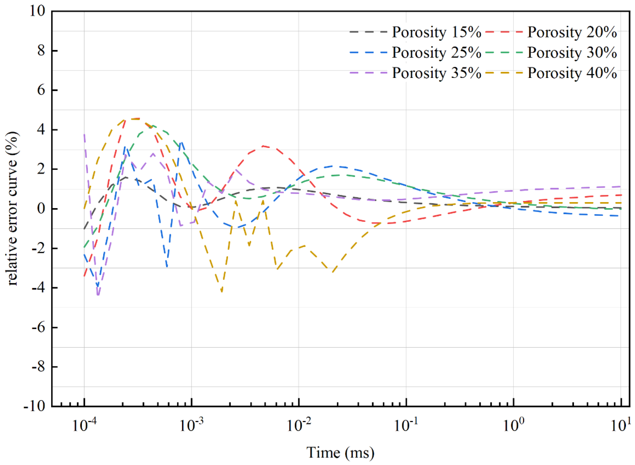
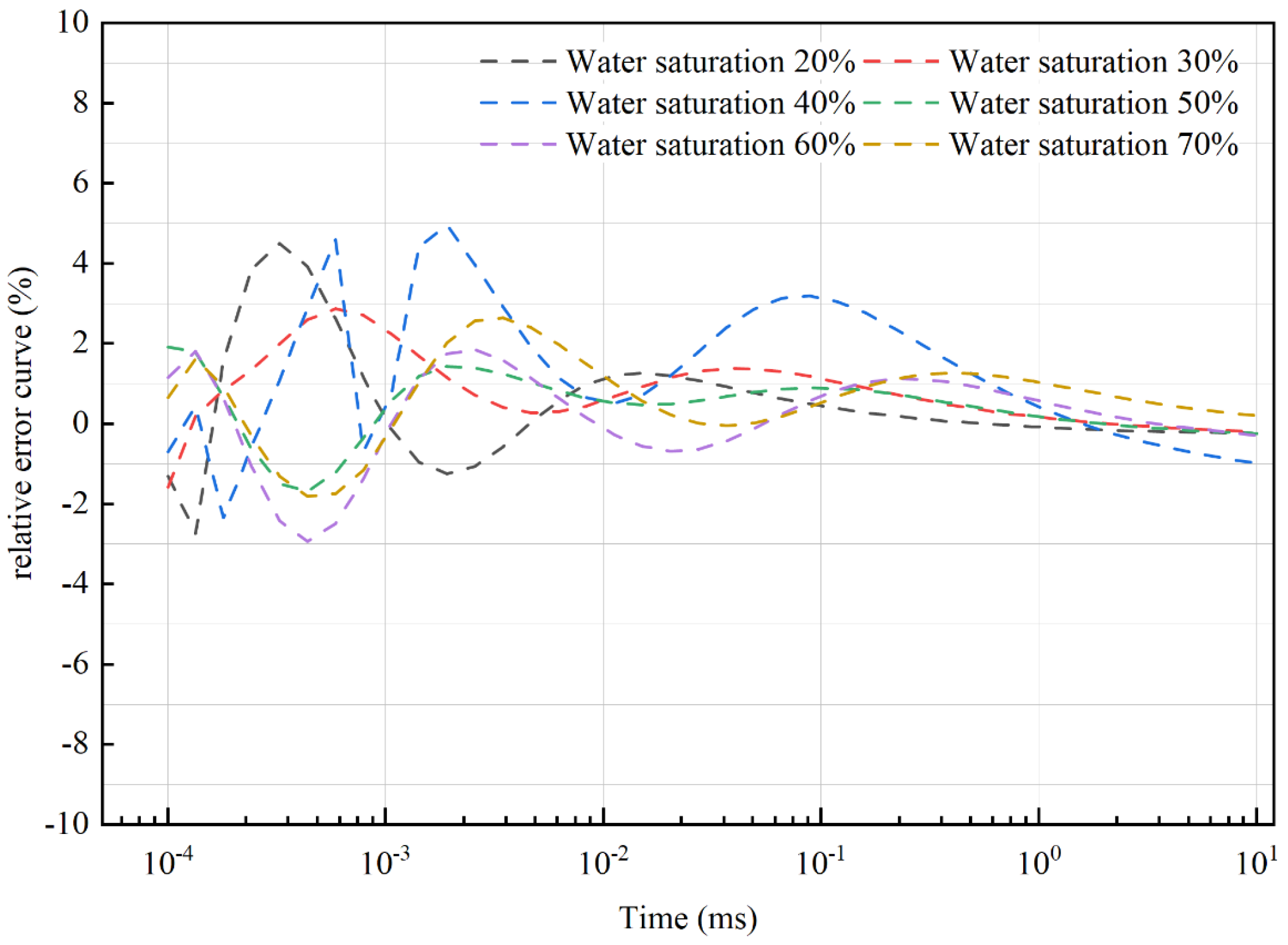
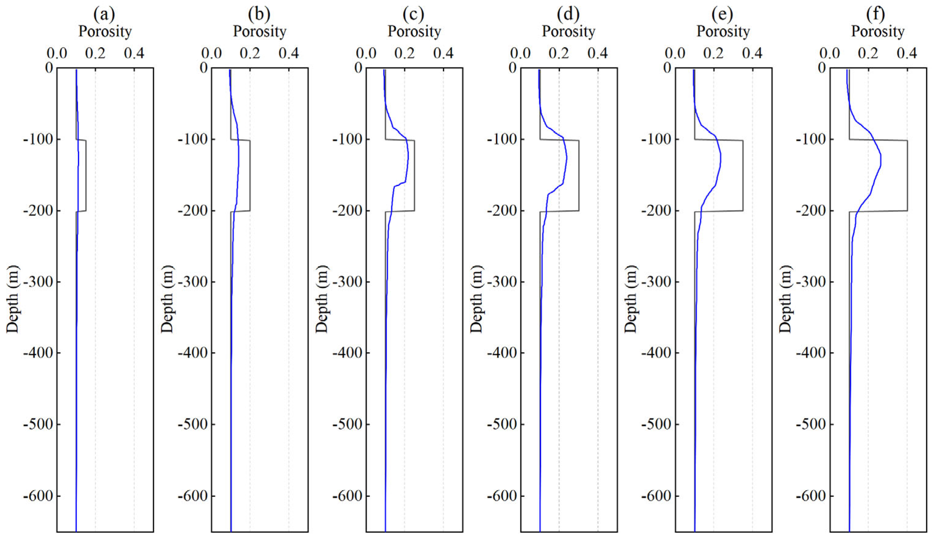
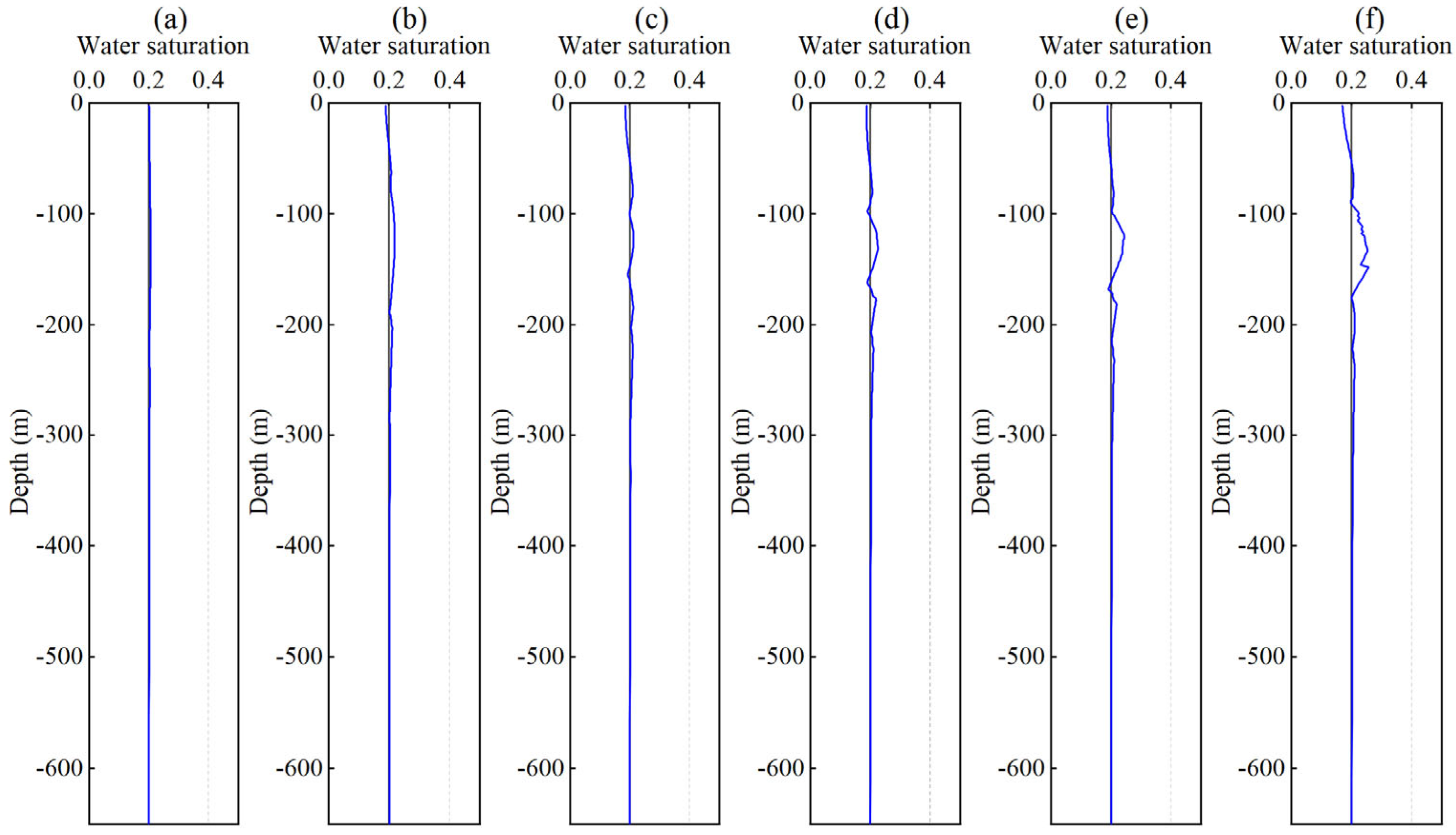
To enhance the geological interpretability of transient electromagnetic (TEM) inversion results, this study proposes a method for directly inverting rock physical parameters based on Archie’s equation. By incorporating porosity and water saturation into the inversion objective function, the formation of petrophysical parameters can be directly retrieved from the TEM data. To verify the validity and feasibility of the proposed method, a series of geoelectric models with varying porosities and water saturation values were constructed and tested using numerical simulations.

(2)

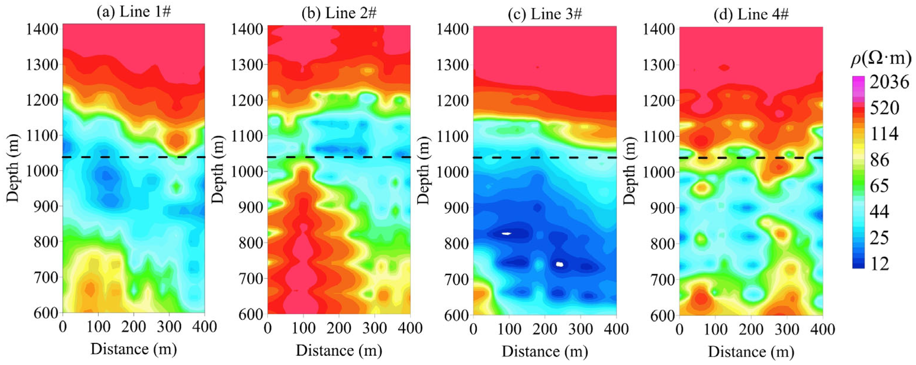
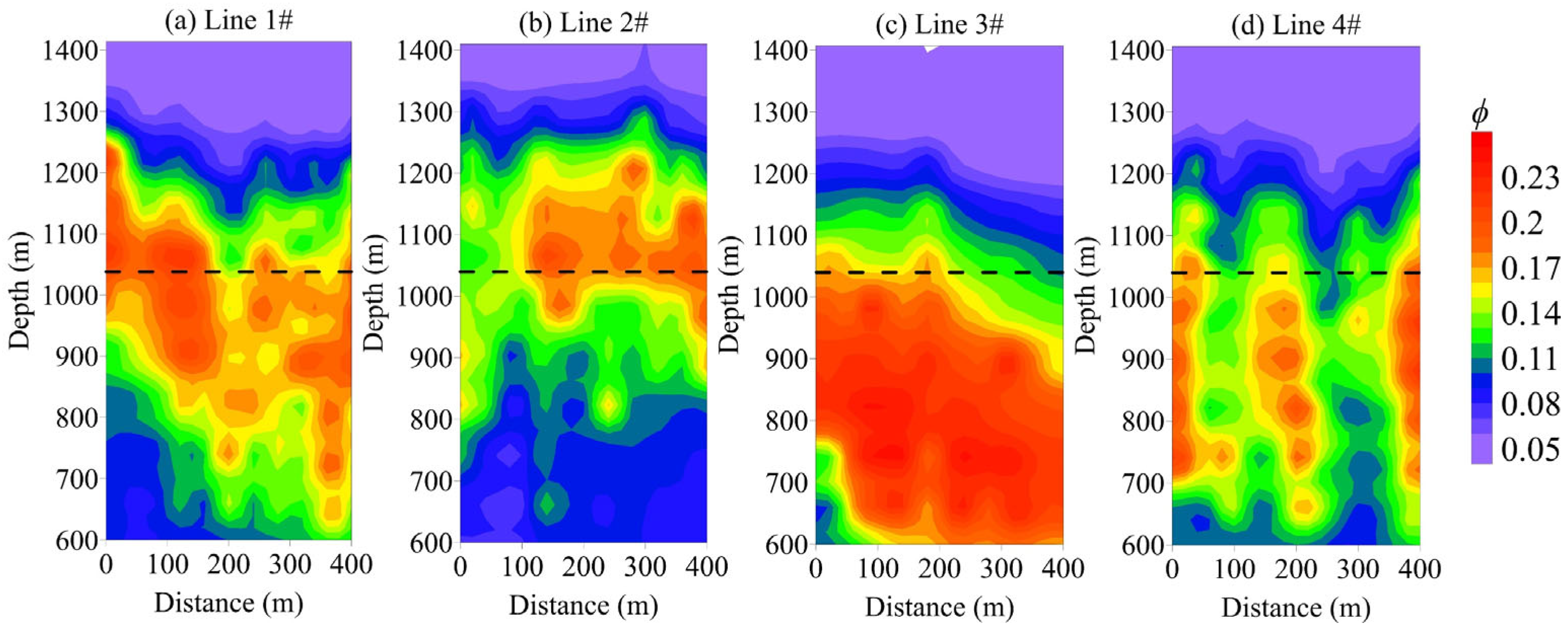
The proposed method was applied to surface transient electromagnetic (TEM) surveys at the 8311 working face of the Tongxin Coal Mine. The spatial distribution of water saturation and porosity was determined by integrating subsurface electromagnetic responses with geological data. These results provide a scientific basis for the fine-scale characterization of coal and rock physical properties and for understanding the development patterns of pores and fractures in underground strata.

(3)

Due to the inherent non-uniqueness of inversion results and the limited applicability of Archie’s equation, errors may be introduced into the inversion of petrophysical parameters. To improve the accuracy of geological interpretation, it is recommended to establish a site-specific petrophysical constitutive relationship for the target exploration area prior to the inversion. This approach reduces the number of unknown parameters and enhances the model constraints, thereby improving the reliability of the inversion results.

References

1. Xue, G.Q.; Yu, J.C. New development of TEM research and application in coal mine exploration. Prog. Geophys. 2017, 32, 319–326. [Google Scholar]
2. Yue, J.H.; Xue, G.Q. Review on the development of Chinese coal electric and electromagnetic prospecting during past 36 years. Prog. Geophys. 2016, 31, 1716–1724. [Google Scholar]
3. Glover, P.W.J. A generalized Archie’s law for n phases. Geophysics 2010, 75, E247–E265. [Google Scholar] [CrossRef]
4. Cai, J.C.; Wei, W.; Hu, X.Y.; Wood, D.A. Electrical conductivity models in saturated porous media: A review. Earth-Sci. Rev. 2017, 171, 419–433. [Google Scholar] [CrossRef]
5. Zhang, Z.S. Theoretical roots of Archie formulas. Prog. Geophys. 2020, 35, 1514–1522. [Google Scholar]
6. Sun, D.M.; Chu, R.J. A theoretical and experimental study for saturation exponent, n. Acta Petrolei Sinica 1994, 15, 66. [Google Scholar]
7. Nakamura, M.; Kusumi, H. An estimation method of in-situ rock masses by characteristic of electric resistivity for jointed rock mass model. Zairyo 2006, 55, 458. [Google Scholar]
8. Nakamura, M.; Kusumi, H.; Kondo, E. Application of several electric resistivities of rock masses for tunnel supporting design. In Modern Tunneling Science and Technology; Routledge: London, UK, 2017; pp. 273–276. [Google Scholar]
9. Coli, N.; Pranzini, G.; Alfi, A.; Boerio, V. Evaluation of rock-mass permeability tensor and prediction of tunnel inflows by means of geostructural surveys and finite element seepage analysis. Eng. Geol. 2008, 101, 174–184. [Google Scholar] [CrossRef]
10. Montaron, B. Connectivity theory—A new approach to modeling non-Archie rocks. Petrophysics 2009, 50, SPWLA-2009-v50n2a2. [Google Scholar]
11. Yang, Q.S.; Torres-Verdín, C. Joint interpretation and uncertainty analysis of petrophysical properties in unconventional shale reservoirs. Interpretation 2015, 3, SA33–SA49. [Google Scholar] [CrossRef]
12. Jin, Y.R.; Li, S.X.; Yang, D.Y. Experimental and theoretical quantification of the relationship between electrical resistivity and hydrate saturation in porous media. Fuel 2020, 269, 117378. [Google Scholar] [CrossRef]
13. Li, H.; Xue, G.Q.; Zhou, N.N.; Chen, W.Y. Appraisal of an array TEM method in detecting a mined-out area beneath a conductive layer. Pure Appl. Geophys. 2015, 172, 2917–2929. [Google Scholar] [CrossRef]
14. Fan, T.; Qi, Z.P.; Yan, B.; Zhao, Z.; Wang, B.; Shi, X.; Liu, L.; Zhao, R.; Wang, J.; Li, B.; et al. Full waveform inversions of borehole transient electromagnetic virtual wave fields and potential applications. J. Environ. Eng. Geoph. 2020, 25, 211–222. [Google Scholar]
15. Wang, P.; Yao, W.H.; Guo, J.L.; Su, C.; Wang, Q.; Wang, Y.; Zhang, B.; Wang, C. Detection of shallow buried water-filled goafs using the fixed-loop transient electromagnetic method: A case study in Shaanxi, China. Pure Appl. Geophys. 2021, 178, 529–544. [Google Scholar] [CrossRef]
16. Kafri, U.; Goldman, M. The use of the time domain electromagnetic method to delineate saline groundwater in granular and carbonate aquifers and to evaluate their porosity. J. Appl. Geophys. 2005, 57, 167–178. [Google Scholar] [CrossRef]
17. Choi, J.S.; Ryu, H.H.; Lee, I.M.; Cho, G.C. Rock mass classification using electrical resistivity-An analytical study. KEM 2006, 321, 1411–1414. [Google Scholar] [CrossRef]
18. Chen, K.; Xue, G.Q.; Chen, W.Y.; Zhou, N.N.; Li, H. Fine and quantitative evaluations of the water volumes in an aquifer above the coal seam roof, based on TEM. Mine Water Environ. 2019, 38, 49–59. [Google Scholar] [CrossRef]
19. Killingbeck, S.F.; Booth, A.D.; Livermore, P.W.; Bates, C.R.; West, L.J. Characterisation of subglacial water using a constrained transdimensional Bayesian transient electromagnetic inversion. Solid Earth 2020, 11, 75–94. [Google Scholar] [CrossRef]
20. Killingbeck, S.F.; Dow, C.F.; Unsworth, M.J. A quantitative method for deriving salinity of subglacial water using ground-based transient electromagnetics. J. Glaciol. 2022, 68, 319–336. [Google Scholar] [CrossRef]
21. Cheng, J.L.; Wang, H.J.; Xu, Z.Z.; Huang, Q.S.; Jiang, G.Q. Research on aquifer water abundance evaluation by borehole transient electromagnetic method based on FCNN. Coal Geol. Explor. 2023, 51, 26. [Google Scholar]
22. Rajab, J.A.; El-Kaliouby, H.; Tarazi, E.A.; Al-Amoush, H. Multiscale geoelectrical characteristics of seawater intrusion along the eastern coast of the Gulf of Aqaba, Jordan. J. Appl. Geophys. 2023, 208, 104868. [Google Scholar] [CrossRef]
23. Faghih, Z.; Haroon, A.; Jegen, M.; Gehrmann, R.; Schwalenberg, K.; Micallef, A.; Dettmer, J.; Berndt, C.; Mountjoy, J.; Weymer, B.A. Characterizing offshore freshened groundwater salinity patterns using trans-dimensional Bayesian inversion of controlled source electromagnetic data: A case study from the Canterbury Bight, New Zealand. Water Resour. Res. 2024, 60, e2023WR035714. [Google Scholar] [CrossRef]
24. Zhang, H.; Xue, B.Q.; Liu, X.G.; Wei, J.; Ding, R.; Zhao, Y.; Liang, L.; Jia, Z. Study on the Relationship between Lithological Differences and Electromagnetic Changes during Mine Water Inrush. Lithosphere 2025, 2025, lithosphere_2024_184. [Google Scholar] [CrossRef]
25. Rupesh, R.; Tiwari, P.; Sharma, S.P. Estimation of geotechnical parameters for coal exploration from Quasi-3D electrical resistivity measurements. Minerals 2024, 14, 102. [Google Scholar] [CrossRef]
26. Fasihi, R.; Tizro, A.T.; Marofi, S.; Voudouris, K. Comparative studies of electromagnetic and geoelectrical methods to estimate the porosity and specific yield of karst aquifer, West of Iran. Environ. Earth Sci. 2024, 83, 469. [Google Scholar] [CrossRef]
27. Ahmed, A.; Deleersnyder, W.; Dudal, D.; Hermans, T. Stochastic inversion of the fresh-/saltwater interface from electromagnetic data. In Proceedings of the Geologica Belgica–Luxemburga International Meeting, Liège, Belgium, 11–13 September 2024. [Google Scholar]
28. Ahmed, A.; Aigner, L.; Michel, H.; Deleersnyder, W.; Dudal, D.; Flores Orozco, A.; Hermans, T. Assessing and improving the robustness of bayesian evidential learning in one dimension for inverting TDEM data: Introducing a new threshold procedure. Water 2024, 16, 1056. [Google Scholar] [CrossRef]
29. Bou-Rabee, F.; Yogeshwar, P.; Burberg, S.; Tezkan, B.; Duane, M.; Ibraheem, I.M. Imaging of groundwater salinity and seawater intrusion in Subiya Peninsula, Northern Kuwait, using transient electromagnetics. Water 2025, 17, 652. [Google Scholar] [CrossRef]
30. Xie, H.J.; Guo, Y.F.; Li, G.Y.; Li, J.R.; Liu, R.Q.; Liang, Y.Q. Laterally constrained inversion of time-domain transient electromagnetic data and using it for detecting water-rich zones in coal mines. Mine Water Environ. 2025, 1–11. [Google Scholar] [CrossRef]
31. Xue, G.Q.; Li, X.; Di, Q.Y. The progress of TEM in theory and application. Prog. Geophys. 2007, 22, 1195–1200. [Google Scholar]
32. Zhdanov, M.S. Foundations of Geophysical Electromagnetic Theory and Methods; Elsevier Science: Amsterdam, The Netherlands, 2017. [Google Scholar]
33. Zhdanov, M.S. Geophysical Inverse Theory and Regularization Problems; Elsevier Science: Amsterdam, The Netherlands, 2002. [Google Scholar]
34. Archie, G.E. The electrical resistivity log as an aid in determining some reservoir characteristics. Trans. AIME 1942, 146, 54–62. [Google Scholar] [CrossRef]
Figure 1. Schematic diagram of the working mode of the transient electromagnetic method.
Applsci 15 06256 g001
Figure 2. Geoelectric models corresponding to different porosity values: (a) 15%, (b) 20%, (c) 25%, (d) 30%, (e) 35%, and (f) 40%.
Applsci 15 06256 g002
Figure 3. Geoelectric models corresponding to different water saturation values: (a) 20%, (b) 30%, (c) 40%, (d) 50%, (e) 60%, and (f) 70%.
Applsci 15 06256 g003
Figure 4. Magnetic field response curve when porosity changes. (a) porosity 15%, (b) porosity 20%, (c) porosity 25%, (d) porosity 30%, (e) porosity 35%, and (f) porosity 40%.
Applsci 15 06256 g004
Figure 5. Magnetic field response error curve when the porosity changes.
Applsci 15 06256 g005
Figure 6. Magnetic field response curve when the water saturation changes. (a) water saturation 20%, (b) water saturation 30%, (c) water saturation 40%, (d) water saturation 50%, (e) water saturation 60%, and (f) water saturation 70%.
Applsci 15 06256 g006
Figure 7. Magnetic field response error curve when the water saturation changes.
Applsci 15 06256 g007
Figure 8. Resistivity inversion results corresponding to different porosity values: (a) 15%, (b) 20%, (c) 25%, (d) 30%, (e) 35%, and (f) 40%.
Applsci 15 06256 g008
Figure 9. Resistivity inversion results corresponding to different water saturation values: (a) 20%, (b) 30%, (c) 40%, (d) 50%, (e) 60%, and (f) 70%.
Applsci 15 06256 g009
Figure 10. Porosity inversion results for different porosity values: (a) 15%, (b) 20%, (c) 25%, (d) 30%, (e) 35%, and (f) 40%.
Applsci 15 06256 g010
Figure 11. Water saturation inversion results for Sw = 20%. (a) porosity 15%, (b) porosity 20%, (c) porosity 25%, (d) porosity 30%, (e) porosity 35%, and (f) porosity 40%.
Applsci 15 06256 g011
Figure 12. Water saturation inversion results for different saturation values: (a) 20%, (b) 30%, (c) 40%, (d) 50%, (e) 60%, and (f) 70%.
Applsci 15 06256 g012
Figure 13. Inversion result for porosity φ = 20%. (a) water saturation 20%, (b) water saturation 30%, (c) water saturation 40%, (d) water saturation 50%, (e) water saturation 60%, and (f) water saturation 70%.
Applsci 15 06256 g013
Figure 14. Exploration area location and survey line layout.
Applsci 15 06256 g014
Figure 15. Multi-channel-induced electromotive force curves: (a) Line 1, (b) Line 2, (c) Line 3, (d) Line 4.
Applsci 15 06256 g015
Figure 16. Inversion resistivity cross-section: (a) Line 1, (b) Line 2, (c) Line 3, (d) Line 4.
Applsci 15 06256 g016
Figure 17. Inversion porosity cross section: (a) Line 1, (b) Line 2, (c) Line 3, (d) Line 4.
Applsci 15 06256 g017
Figure 18. Inversion water saturation cross-section: (a) Line 1, (b) Line 2, (c) Line 3, (d) Line 4.
Applsci 15 06256 g018
Disclaimer/Publisher’s Note: The statements, opinions and data contained in all publications are solely those of the individual author(s) and contributor(s) and not of MDPI and/or the editor(s). MDPI and/or the editor(s) disclaim responsibility for any injury to people or property resulting from any ideas, methods, instructions or products referred to in the content.