Evaluation of Correlation-Based Methods for Time Period Estimation in Vehicle Speed Measurement Using Pyroelectric Infrared Sensors

Abstract

Accurate time period estimation (TPE) between sensor signals is essential for vehicle speed measurement in intelligent transportation systems (ITSs). In this context, we focus on time period estimation using signals acquired from a dual pyroelectric infrared (PIR) sensor setup. To estimate the time period between these signals, this paper analyzes and compares two correlation-based methods—conventional cross-correlation (CCF) and Hilbert transform-enhanced cross-correlation (CCFHT). An analytical framework is developed to quantify the bias and variance of each method under practical conditions, including sensor mismatch and noise. The PIR sensor signals are modeled based on their dynamic response characteristics, enabling theoretical analysis supported by simulations and field experiments. Results show that although both methods yield negligible bias under ideal conditions, CCFHT significantly reduces estimation variance in noisy or mismatched scenarios. These findings confirm the advantages of CCFHT for achieving robust and precise vehicle speed estimation using low-cost PIR sensor systems, and provide insights into practical deployment within ITSs.

1. Introduction

1.1. Background

Accurate and reliable vehicle speed measurement is a fundamental component of intelligent transportation systems (ITSs), serving critical applications such as traffic flow analysis, congestion monitoring, incident detection, and automated enforcement [1]. Among the commonly used methods for speed measurement, time delay in the literature [2,3,4]) estimation (TPE) between two spatially separated sensors remains one of the most intuitive and robust strategies, especially for point-based systems [5,6]. This approach estimates the travel time of a vehicle between two sensor units to compute speed from the known baseline distance. However, the performance of TPE critically depends on the quality and consistency of the signals acquired from both sensors.

Various technologies have been employed for vehicle detection and TPE, including radar, LiDAR, magnetic loops, and video cameras [7,8,9,10]. These methods, which are supposed to be accurate, often suffer from high deployment costs, power demands, or environmental limitations. In contrast, pyroelectric infrared (PIR) sensors provide a low-cost, passive, and energy-efficient alternative, particularly suited for scenarios where minimal infrastructure is preferred or energy constraints exist [11,12].

PIR sensors detect changes in infrared radiation, typically emitted by heating objects such as vehicles when they pass through the sensors’ fields of view (FOV) and convert them into electrical signals. When a group of two or more PIR sensors are placed along a lane at a known distance apart, the time period or time interval between their response signals can be used to estimate vehicle speed. Despite their simplicity, PIR-based speed measurement systems face several challenges for TPE: variability in sensor response time due to differing thermal or electrical time constants; environmental noise and reflections, which degrade the signal-to-noise ratio; limited temporal resolution, which hinders precision in fast or closely spaced events.

These challenges lead to the need for a deeper understanding of how sensor imperfections and signal characteristics affect the accuracy of TPE, particularly through systematic error analysis.

1.2. Related Work

Time period or time delay estimation has been widely studied in applications such as radar, seismology, audio processing, and biomedical signal analysis [13,14,15]. The conventional cross-correlation function (CCF) remains one of the most popular methods for estimating the time shift between signals [16,17,18]. However, it is known to be sensitive to noise, signal distortion, and amplitude variations, which may reduce accuracy in practical implementations [19,20]. To address these issues, enhanced methods such as CCF enhanced with Hilbert transform (CCFHT) have been proposed, leveraging the analytic signal representation to improve phase alignment and robustness [21,22,23]. These methods offer a balance between computational efficiency and improved estimation accuracy under noise conditions.

In the context of vehicular sensing, PIR sensors have been used in basic applications such as motion detection, vehicle counting, and lane occupancy. However, in most speed-related applications [11,12,24], the emphasis is often on straightforward delay measurement rather than a detailed analysis of signal behavior or estimation uncertainty. Even in our previous work [25], a prototype PIR-based speed measurement system was introduced, and speed was estimated using threshold and analog signal processing techniques. While the system demonstrated feasibility, it lacked a comprehensive evaluation of accuracy, bias, and variance in the time estimation process.

To the best of our knowledge, no prior study has systematically evaluated the application of correlation-based estimators—such as CCF and CCFHT—to PIR-based speed measurement systems under conditions involving sensor response mismatch and environmental noise. This gap motivates the need for a dedicated framework to analyze estimation performance in such systems.

1.3. Contributions

This paper focuses on evaluating the cross-correlation fFunction (CCF) and cross-correlation function with Hilbert transform (CCFHT) for TPE in PIR sensor-based vehicle speed measurement. The specific contributions of this work are as follows:

-

A detailed mathematical evaluation of conventional and enhanced cross-correlation methods for TPE.

-

An investigation into sensor response divergence and its effects on estimation accuracy.

-

A numerical analysis of system parameters—including bandwidth, signal-to-noise ratio (SNR), and sensor time constants—to assess their influence on time period estimation performance, complemented by limited experimental validation to compare the overall performance of CCF and CCFHT.

By integrating theoretical modeling, simulation, and real-world validation, this study provides practical insights into the performance and limitations of low-cost PIR-based vehicle speed sensing, laying the foundation for future ITS applications that require robust and lightweight estimation techniques.

2. Materials and Methods

This section presents the analytical and modeling framework developed to evaluate the bias and variance of time period estimation methods applied to PIR sensor signals. The objective is to provide a systematic and quantifiable analysis of how estimation errors are affected by sensor imperfections, signal characteristics, and system parameters. The structure of this section follows logical progression:

-

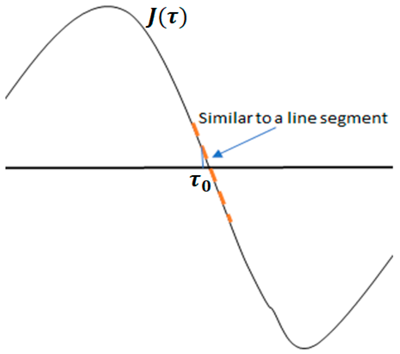
Section 2.1 introduces the general bias and variance analysis framework for zero-point estimators, derived mean value theorem, or Taylor expansion.

-

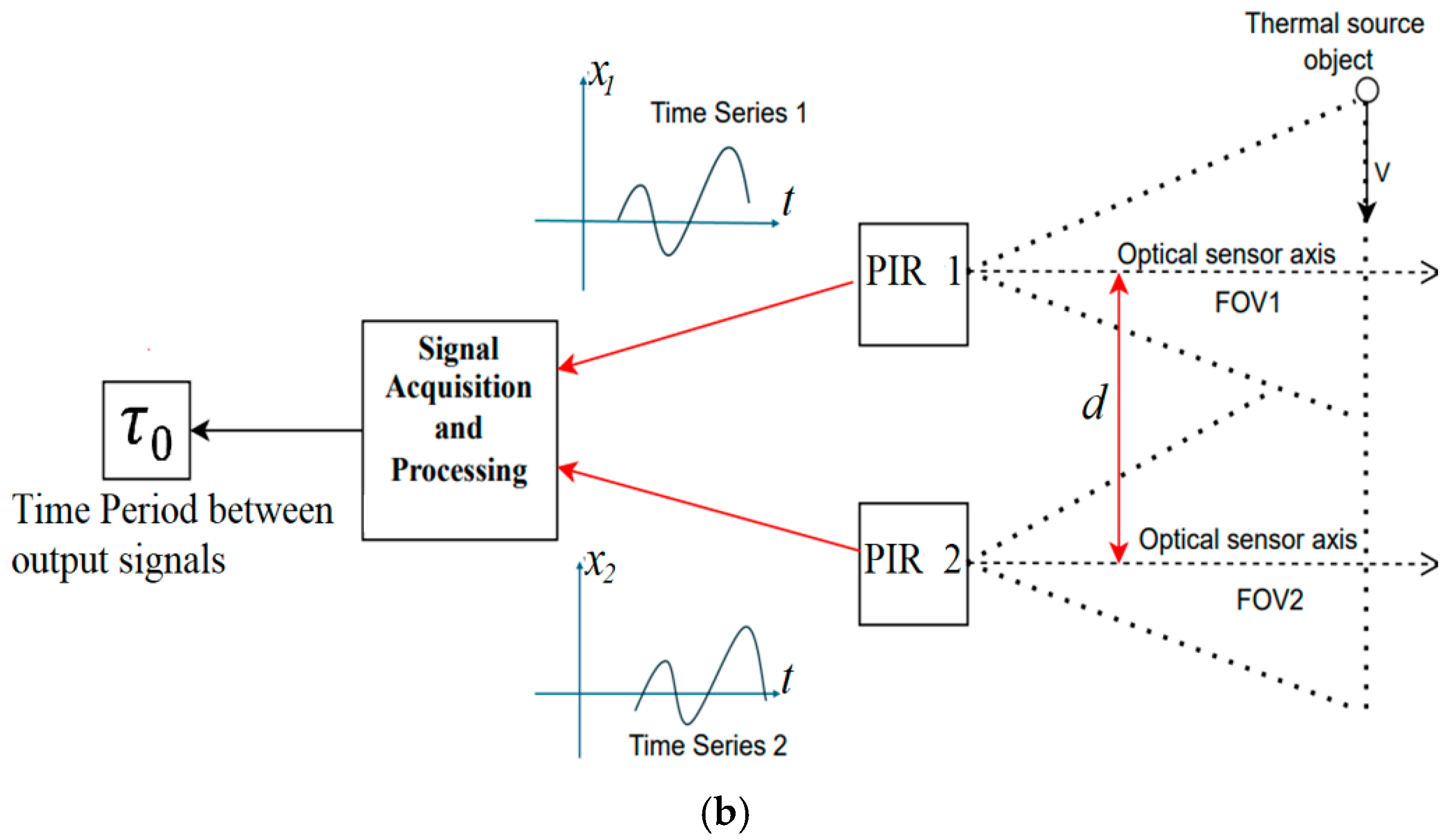
Section 2.2 describes the signal modeling of PIR sensors in the context of vehicle speed measurement, highlighting waveform characteristics and inter-sensor mismatches.

-

Section 2.3 and Section 2.4 apply the general framework to two specific correlation-based estimators—conventional cross-correlation function (CCF) and Hilbert-enhanced CCF (CCFHT)—to derive analytical expressions for their expected bias and variance under various conditions.

2.1. Analytical Framework for Bias and Variance Analysis of Estimators

In order to evaluate the estimation biases and uncertainties using traditional cross-correlation function and CCF combined with Hilbert transform, we employ the zero-point estimation analysis. Let $J\left(\tau \right)$ be the objective function and we have to find the zero point ${\tau }_0$ such that $J\left({\tau }_0\right)=0$, in the scene that the measured $J\left(\tau \right)$ might contain some noise. Suppose its estimated value is $\widehat{{\tau }_0}$, using the mean value theorem, or similarly the Taylor expansion [26]:

$$0=J(\widehat{{\tau }_0} )=J\left({\tau }_0\right)+(\widehat{{\tau }_0}-{\tau }_0 ) J^{\prime } \left({\tau }_{\xi }\right)$$

(1)

for some ${\tau }_{\xi }$ lying between ${\tau }_0$ and $\widehat{{\tau }_0}$. Thus:

$$\begin{gathered} (\widehat{{\tau }_0}-{\tau }_0 ) J^{\prime } \left({\tau }_{\xi }\right)=J(\widehat{{\tau }_0} ) \\ \mathrm{and} {\left(\widehat{{\tau }_0}-{\tau }_0\right)}^2\times J^{\prime } {\left({\tau }_{\xi }\right)}^2=J{\left({\tau }_0\right)}^2 \end{gathered}$$

(2)

In many practical cases, the objective function $J\left(\tau \right)$ is usually smooth around the point ${\tau }_0$ (Figure 1), so that $J^{\prime }\left(\tau \right)\approx J^{\prime }\left({\tau }_0\right)$, and accordingly, $\mathbb{E}\left[J^{\prime }\right(\tau \left)\right]\approx \mathbb{E}\left[J^{\prime }\right({\tau }_0\left)\right]$ for $\tau$ close to ${\tau }_0$. Here, denote $\mathbb{E}\left[x\right]$ to be the expected value of a random variable x. Thus:

$$\begin{gathered} -\mathbb{E}\left[J\left({\tau }_0\right)\right]=\mathbb{E}\left[\left(\widehat{{\tau }_0}-{\tau }_0\right)J^{\prime }\left({\tau }_{\xi }\right)\right] \approx \mathbb{E}\left[\left(\widehat{{\tau }_0}-{\tau }_0\right)\right]·\mathbb{E}\left[J^{\prime }\left({\tau }_0\right)\right] \\ \mathrm{and} \mathbb{E}\left[J{\left({\tau }_0 \right)}^2\right]=\mathbb{E}[{\left(\widehat{{\tau }_0}-{\tau }_0\right)}^2·J^{\prime }{\left({\tau }_{\xi }\right)}^2]\approx \mathbb{E}\left[{\left(\widehat{{\tau }_0}-{\tau }_0\right)}^2\right]·\mathbb{E}{\left[J^{\prime }\left({\tau }_0\right)\right]}^2 \end{gathered}$$

(3)

Consequently, the definition of bias and variance of the zero-point estimation are defined as:

$$bias \left(\widehat{{\tau }_0}\right)=\mathbb{E}\left[\right(\widehat{{\tau }_0}-{\tau }_0\left)\right]\approx -{\displaystyle \frac{\mathbb{E}\left[J\left({\tau }_0\right)\right]}{\mathbb{E}\left[J^{\prime }\left({\tau }_0\right)\right]}}$$

(4)

$$var \left(\widehat{{\tau }_0}\right)=\mathbb{E}\left[{\left(\widehat{{\tau }_0}-{\tau }_0\right)}^2\right]\approx {\displaystyle \frac{\mathbb{E}\left[J{\left({\tau }_0\right)}^2\right]}{\mathbb{E}{\left[J^{\prime }\left({\tau }_0\right)\right]}^2}}$$

(5)

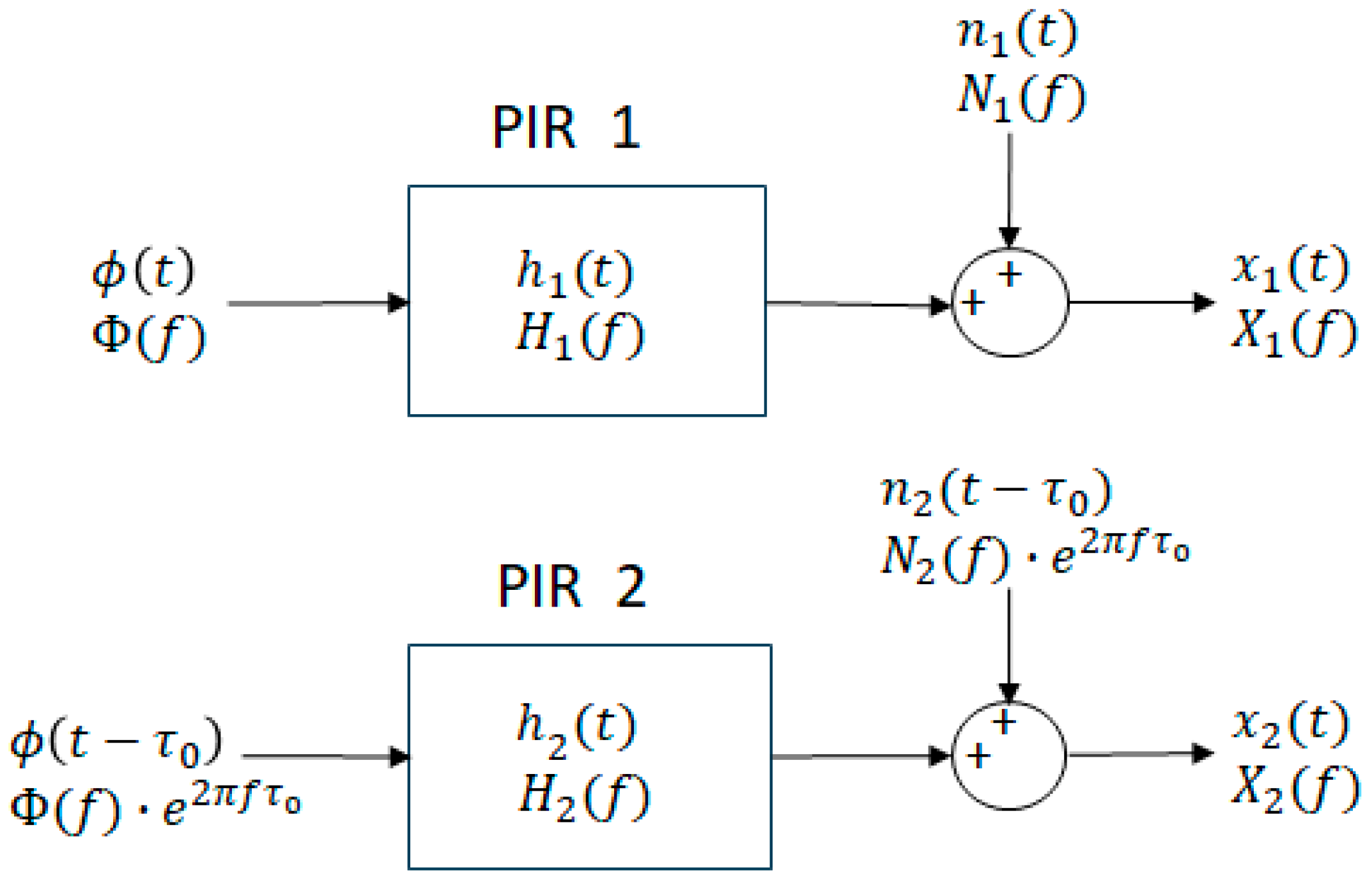
2.2. PIR Signal Modeling for Time Period Estimation

To apply the above framework to vehicle speed estimation using PIR sensors, we model the signal behavior of the sensors as a vehicle passes through their fields of view. In this study, a vehicle speed measurement is designed using two pyroelectric infrared (PIR) sensor modules placed in a known geometric configuration (Figure 2a). The system is designed to minimize centering errors by ensuring the parallel alignment between the optical axes of the sensor modules and maintaining an accurate distance d between the FOV center axes of the sensors [27,28]. As a vehicle moves past these sensors, it causes changes in the sensors’ output signals, which are then analyzed to estimate time delay between the two signals and consequently to determine the speed of the moving vehicle (Figure 2b).

The fundamental principle behind this system is that the time period between the sensor outputs can be used to compute speed using the equation:

$$v=d/{\tau }_0$$

(6)

where ${\tau }_0$ is the time period between their output signals.

To analyze the performance of different TPE methods, we first define the mathematical representation of the signals. The two output signals of the PIR sensors over a monitoring window [0, T] can be modeled as $x_1\left(t\right)$ and $x_2\left(t\right)$ for 0 ≤ t ≤ T, where $x_2\left(t\right)$ is essentially a time-shifted version of $x_1\left(t\right)$: $x_2\left(t\right) ~ x_1(t-{\tau }_0)$.

Table 1. Time and frequency domain notations of quantities related to PIR sensor signals.

Quantity	Notation in Time Domain	Notation in Frequency Domain
Difference between infrared fluxes from the interested object incoming on 2 elements of PIR sensor	$\varphi \left(t\right)$	$\mathsf{\Phi }\left(f\right)$
Impulse response of PIR 1	$h_1\left(t\right)$	$H_1\left(f\right)$
Impulse response of PIR 2	$h_2 \left(t\right)$	$H_2\left(f\right)$
Output signal of PIR 1	$x_1\left(t\right)$	$X_1\left(f\right)$
Output signal of PIR 2	$x_2\left(t\right)$	$X_2\left(f\right)$
Noise signal at PIR 1	$n_1\left(t\right)$	$N_1\left(f\right)$
Noise signal at PIR 2	$n_2\left(t\right)$	$N_2\left(f\right)$

presents notations of several quantities related to PIR sensor signals that are used in this analysis.

In PIR sensor-based speed measurement, the differential infrared flux detected by the two sensing elements of each PIR sensor is denoted as a function over time $\varphi \left(t\right)$ [29,30]. This flux variation is caused by the movement of a heat emitting object (vehicle) across the sensor’s FOV. If we define the differential flux from the object for the first sensor as $\varphi \left(t\right)$, the second sensor $\varphi (t-{\tau }_0)$. As a moving heat source (e.g., a vehicle) passes through the sensor’s field of view (FOV), the incident infrared radiation varies over time, producing a structured alternating signal due to the differential sensing mechanism. Given that vehicles typically follow a consistent motion trajectory within the monitored region, the resulting $\varphi \left(t\right)$ can be approximated as a sinusoidal signal within the observation window. This sinusoidal assumption is justified by the periodic nature of the sensor’s response to smoothly moving sources and enables a more tractable mathematical representation for time period estimation. Treating $\varphi \left(t\right)$ as a sinusoid simplifies its frequency domain analysis, allows the use of Fourier-based techniques, and enhances computational efficiency in estimating time period via cross-correlation methods.

$$\begin{gathered} \varphi \left(t\right)={\varphi }_0·\sin \left(2\pi f_{0}t\right) \\ \Phi \left(f\right)={\displaystyle \frac{{\varphi }_0}{2j}}\delta \left(f-f_0\right)-{\displaystyle \frac{{\varphi }_0}{2j}}\delta \left(f+f_0\right) \end{gathered}$$

(7)

Each PIR sensor operates as a linear system with a transfer function $H_i\left(s\right)$ and impulse response $h_i\left(t\right) (i=1, 2)$ (Figure 3). Consequently, output signals of the PIR sensors can be established in such a way that:

$$\begin{gathered} x_1\left(t\right)=h_1\left(t\right)⨂\varphi \left(t\right)+n_1\left(t\right) \\ {x}_2\left(t\right)=h_2\left(t\right)⨂\varphi (t-{\tau }_0)+n_2(t-{\tau }_0) \end{gathered}$$

(8)

Using the Laplace transform, the system equations in the frequency domain can be written as:

$$\begin{array}{l}{X}_1\left(f\right)=H_1\left(f\right)·\Phi \left(f\right)+N_1\left(f\right)\\ X_2\left(f\right)=\left(H_2\left(f\right)·\Phi \left(f\right)+N_2\left(f\right)\right)e^{j2\pi f{\tau }_0}\end{array}$$

(9)

For practical PIR sensor systems, the transfer function is often modeled as a second-order system [30,31]:

$$H_i\left(s\right)={\displaystyle \frac{A_{i}s}{\left(1+{\tau }_{th.i}s\right)\left(1+{\tau }_{e.i}s\right)}} for i=\mathrm{1,2}$$

(10)

where parameters ${\tau }_{th.i},{\tau }_{e.i}$ are thermal time constant and electric time constant and $A_i$ is the gain faction of each sensor i (i = 1, 2).

Noise in PIR sensors primarily arises from thermal fluctuations in the sensing elements, electronic noise in the amplification and filtering stages, environmental interferences from ambient temperature variations, etc. [6]. Assuming the noise signals $n_{1 }\left(t\right),{ n}_2 \left(t\right)$ are white Gaussian noises within the working specific bandwidth [−B, B] of the sensors, they satisfy the following Equations (11)–(15), according to references [14,32,33].

1. Zero-mean:

$$\mathbb{E}\left[n_1\left(t\right)\right]=\mathbb{E}\left[n_2\left(t\right)\right]=0; \mathbb{E}\left[N_1\left(f\right)\right]=\mathbb{E}\left[N_2\left(f\right)\right]=0$$

(11)

2. Independence:

$$\mathbb{E}\left[N_1\left(f_1\right)N_2\left(f_2\right)\right]=0$$

(12)

3. Variance:

$$var\left(n_1\left(t\right)\right)=\mathbb{E}\left[n_1{\left(t\right)}^2\right]={\sigma }_{n1}^2; var\left(n_2\left(t\right)\right)=\mathbb{E}\left[n_2{\left(t\right)}^2\right]={\sigma }_{n2}^2$$

(13)

4. Power Spectral Densities:

$$S_{n1}\left(f\right)={\sigma }_{n1}^2; S_{n2}\left(f\right)={\sigma }_{n2}^2$$

(14)

5. Correlated for identical frequencies:

$$\begin{gathered} \mathbb{E}\left[Re\left\{N_1\left(f_1\right)N_1\left(f_2\right)\right\}\right]=\mathbb{E}\left[Im\left\{N_1\left(f_1\right)N_1\left(f_2\right)\right\}\right]={\displaystyle \frac{{\sigma }_{n1}^2.T}{2}}·\left(\delta \left(f_1-f_2\right)+\delta \left(f_1+f_2\right)\right) \\ \mathbb{E}\left[Re\left\{N_2\left(f_2\right)N_2\left(f_2\right)\right\}\right]=\mathbb{E}\left[Im\left\{N_2\left(f_1\right)N_2\left(f_2\right)\right\}\right]={\displaystyle \frac{{\sigma }_{n2}^2.T}{2}}·\left(\delta \left(f_1-f_2\right)+\delta \left(f_1+f_2\right)\right) \end{gathered}$$

(15)

where $\delta$ is the notation of the Dirac delta function.

These assumptions facilitate the derivation of analytical expressions for bias and variance in TPE. Further in this paper, it is the attempt to explore the effect of divergence between two responding systems of the PIR sensor modules on the biases and uncertainties of the estimations.

2.3. Bias and Variance Analysis with Conventional Cross-Correlation for TPE

Similarly, in many works, the very conventional approach to time period or time delay estimation between sensors’ output signals is using the crosscorrelation function which is defined as:

$$R_{x_1{x}_2}\left(\tau \right)={\int }_0^T{x}_1\left(\alpha \right)x_2\left(\tau -\alpha \right)d\alpha ; for-T\le \tau \le T$$

(16)

Thus, the time period is essentially estimated as:

$${\tau }_0=\arg \underset{-T\le \tau \le T}{\max }{R}_{x_1{x}_2}\left(\tau \right)$$

(17)

Let $y_1\left(t\right)=x_1\left(t\right);\mathrm{ }{y}_2\left(t\right)=x_2(-t)$, thus:

$$y_2\left(t\right)=h_2\left(-t\right)⨂\varphi (-t-{\tau }_0)+n_2\left(-t-{\tau }_0\right)$$

(18)

and in the frequency domain:

$$Y_2\left(f\right)=\left(H_2\left(-f\right)·\mathsf{\Phi }\left(-f\right)+N_2\left(-f\right)\right)e^{j2\pi f{\tau }_0}=\left(H_2^{\ast }\left(f\right){\mathsf{\Phi }}^{\ast }\left(f\right)+N_2^{\ast }\left(f\right)\right)$$

(19)

where $C^{\ast }$ is the denotation of the conjugated complex number of a complex number C.

The cross-correlation function between the two signals $x_1\left(t\right),{ x}_2\left(t\right)$ is then rewritten as:

$$R_{x_1{x}_2}\left(\tau \right)={\int }_0^T{x}_1\left(\alpha \right)x_2\left(\alpha +\tau \right)d\alpha ={\int }_0^T{x}_1\left(\alpha \right)y_2\left(-\tau -\alpha \right)d\alpha =L(-\tau )$$

(20)

$$\mathrm{w}\mathrm{h}\mathrm{e}\mathrm{r}\mathrm{e}: L\left(\tau \right)={\int }_0^T{x}_1\left(\alpha \right)y_2\left(\tau -\alpha \right)d\alpha$$

(21)

Equation (22) drives the Fourier transform of the function $L\left(\tau \right)$, which is defined as:

$$\begin{gathered} X_1\left(f\right)Y_2\left(f\right)=\left(H_1\left(f\right)\mathsf{\Phi }\left(f\right)+N_1\left(f\right)\right)·\left(H_2^{\ast }{\mathsf{\Phi }}^{\ast }\left(f\right)+N_2^{\ast }\left(f\right)\right)e^{j2\pi f{\tau }_0} \\ =\left(D_1\left(f\right)+N_1\left(f\right)\right)\left(D_2^{\ast }\left(f\right)+N_2^{\ast }\left(f\right)\right)·e^{j2\pi f{\tau }_0} \end{gathered}$$

(22)

Here, we denote the deterministic part of the output signal of each sensor in the frequency domain as:

$$\begin{gathered} D_1\left(f\right)=H_1\left(f\right)\mathsf{\Phi }\left(f\right);D_2\left(f\right)=H_2\left(f\right)\mathsf{\Phi }\left(f\right) \\ \mathrm{and:} M\left(f\right)=\left(D_1\left(f\right)+N_1\left(f\right)\right)\left(D_2^{\ast }\left(f\right)+N_2^{\ast }\left(f\right)\right) \end{gathered}$$

(23)

Therefore, $L\left(\tau \right)$ is the inverse Fourier transform of the function $M\left(f\right)·e^{j2\pi f{\tau }_0}$:

$$L\left(\tau \right)={\int }_0^T{x}_1\left(\alpha \right)y_2\left(\tau -\alpha \right)d\alpha ={\int }_{-B}^{B}M\left(f\right)·e^{j2\pi f\left(\tau +{\tau }_0\right)}df$$

(24)

Due to Equation (17), the following estimate is considered:

$$\widehat{{\tau }_0}= \arg \max \left(L\left(-\tau \right)\right) \mathrm{o}\mathrm{r} \widehat{{\tau }_0}=\arg \left({\displaystyle \frac{d}{d\tau }}L\left(-\tau \right)=0\right)$$

(25)

Thus, the objective function is defined as $J_{CCF}\left(\tau \right)={\displaystyle \frac{d}{d\tau }}L(-\tau )$. Now, we proceed with some calculations to apply the analysis mentioned in Section 2.1 for bias and variance estimation.

$$J_{CCF}\left(\tau \right)=-j2\pi {\int }_{-B}^{B}f.M\left(f\right).e^{j2\pi f\left({\tau }_0-\tau \right)}df$$

(26)

$$J_{CCF}\left({\tau }_0\right)=-j2\pi {\int }_{-B}^{B}f.M\left(f\right)df$$

(27)

$$\mathbb{E}\left[J_{CCF}\left({\tau }_0\right)\right]=-j2\pi {\int }_{-B}^{B}f.\mathbb{E}\left[M\left(f\right)\right]df$$

(28)

$$J_{CCF}{\left({\tau }_0\right)}^2=-4{\pi }^2{\int }_{-B}^B{\int }_{-B}^B{f}_1{f}_2.M\left(f_1\right)M\left(f_2\right)d{f}_{1}d{f}_2$$

(29)

$$\mathbb{E}\left[J_{CCF}{\left({\tau }_0\right)}^2\right]=-4{\pi }^2 {\int }_{-B}^B{\int }_{-B}^B{f}_1{f}_2\mathbb{E}\left[M\left(f_1\right)M\left(f_2\right)\right] d{f}_{1}d{f}_2$$

(30)

$$J_{CCF}^{\prime }\left(\tau \right)={\displaystyle \frac{d}{d\tau }}{J}_{CCF}\left(\tau \right)=-4{\pi }^2{\int }_{-B}^B{f}^2.M\left(f\right)e^{j2\pi f\left({\tau }_0-\tau \right)}df$$

(31)

$$J_{CCF}^{\prime }\left({\tau }_0\right)=-4{\pi }^2{\int }_{-B}^B{f}^2.M\left(f\right)df$$

(32)

$$\mathbb{E}\left[J_{CCF}^{\prime }\left({\tau }_0\right)\right]=-4{\pi }^2{\int }_{-B}^B{f}^2.\mathbb{E}\left[J_{CCF}^{\prime }\left({\tau }_0\right)\right]df$$

(33)

Now, we use Equations (11)–(15) to explore the recent formulas, with the notation that $D_1\left(f\right), D_2\left(f\right)$ is zero for any $f\ne \pm f_0$. To perform this, the term $\Delta f$—the frequency resolution—is introduced to manage the effect of the Dirac delta function $\delta$ in an integral. The Dirac delta function is a mathematical idealization that assigns all energy at a single frequency, making direct integration problematic. To resolve this, $\Delta f$ serves as a small frequency resolution element, ensuring the integral remains finite and meaningful in numerical and practical applications. It ensures that computations remain stable and consistent with real-world signal analysis, where measurements always occur over discrete frequency bins [25,26]:

$$\mathbb{E}\left[J_{CCF}\left({\tau }_0\right)\right]=\pi f_0\times \mathrm{I}\mathrm{m} \left\{D_1\left(f_0\right)D_2^{\ast }\left(f_0\right)\right\}.\Delta f$$

(34)

$$\mathbb{E}\left[J_{CCF}^{\prime }\left({\tau }_0\right)\right]=-2{\pi }^2{f}_0^2\times \mathrm{R}\mathrm{e} \left\{D_1\left(f_0\right)D_2^{\ast }\left(f_0\right)\right\}.\Delta f$$

(35)

$$\mathbb{E}{\left[J_{CCF}^{\prime }\left({\tau }_0\right)\right]}^2=4{\pi }^4{\sigma }_{N_1}^2{\sigma }_{N_2}^2.{\displaystyle \frac{f_0^4}{{\Delta }^{2}f}}.SN{R}_1.SN{R}_2.{{\cos }^2\mathsf{\Theta }}_0$$

(36)

$$\begin{array}{l}\mathbb{E}\left[J_{CCF}{\left({\tau }_0\right)}^2\right]=8{\pi }^2{f}_0^2\times I{m}^2\left\{D_1\left(f_0\right)D_2^{\ast }\left(f_0\right)\right\}.{\Delta }^{2}f\\ \hspace{1em}\hspace{1em}\hspace{1em}\hspace{1em}\hspace{1em}\hspace{1em}\hspace{1em}+8{\pi }^2{f}_0^2\left({\left|D_1\left(f_0\right)\right|}^2\left({\displaystyle \frac{{\sigma }_{N2}^2}{2B}}T\right)+{\left|D_2\left(f_0\right)\right|}^2\left({\displaystyle \frac{{\sigma }_{N1}^2}{2B}}T\right)\right).{\Delta }^{2}f\\ \hspace{1em}\hspace{1em}\hspace{1em}\hspace{1em}\hspace{1em}\hspace{1em}\hspace{1em}+{\displaystyle \frac{8B^3{\pi }^2}{3}}\left({\displaystyle \frac{{\sigma }_{N1}^2}{2B}}T\right)\left({\displaystyle \frac{{\sigma }_{N2}^2}{2B}}T\right)\Delta f\end{array}$$

(37)

$$\begin{array}{l}\mathbb{E}\left[J_{CCF}{\left({\tau }_0\right)}^2\right]=8{\pi }^2{\sigma }_{N1}^2{\sigma }_{N2}^2\\ \hspace{1em}\hspace{1em}\hspace{1em}\hspace{1em}\hspace{1em}\hspace{1em}\hspace{1em}\times \{{\displaystyle \frac{f_0^2}{{\Delta }^{2}f}}\times SN{R}_1.SN{R}_2.\cos {\mathsf{\Theta }}_0+{\displaystyle \frac{f_0^2}{2B/T}}\times \left(SN{R}_1+SN{R}_2\right)\\ \hspace{1em}\hspace{1em}\hspace{1em}\hspace{1em}\hspace{1em}\hspace{1em}\hspace{1em}+{\displaystyle \frac{B.\Delta f}{{12\left(1/T\right)}^2}}\}\end{array}$$

(38)

The previous formulas also present ${\mathsf{\Theta }}_0$ as the argument of the complex number $D_1\left(f_0\right)D_2^{\ast } \left(f_0\right)$ and also of $H_1\left(f_0\right)H_2^{\ast } \left(f_0\right)$; and the signal-to-noise ratios, which present the ratio between the power spectral of the deterministic part over noise:

$$\begin{gathered} SN{R}_1={\displaystyle \frac{{\int }_{-B}^B{\left|D_1\left(f\right)\right|}^{2}df}{{\int }_{-B}^B{\left|N_1\left(f\right)\right|}^{2}df}}={\displaystyle \frac{{\left|D_1\left(f_0\right)\right|}^2.{\Delta }^{2}f}{{\sigma }_{n_1}^2}}; \\ SN{R}_2={\displaystyle \frac{{\int }_{-B}^B{\left|D_2\left(f\right)\right|}^{2}df}{{\int }_{-B}^B{\left|N_2\left(f\right)\right|}^{2}df}}={\displaystyle \frac{{\left|D_2\left(f_0\right)\right|}^2.{\Delta }^{2}f}{{\sigma }_{n_2}^2}} \end{gathered}$$

(39)

Therefore, by applying Formulas (4) and (5), the bias and variance of the estimation are derived as:

$$bias {\left(\widehat{{\tau }_0}\right)}_{CCF}=-{\displaystyle \frac{\mathbb{E}\left[J_{CCF}\left({\tau }_0\right)\right]}{\mathbb{E}\left[J_{CCF}^{\prime }\left({\tau }_0\right)\right]}}=-{\displaystyle \frac{1}{2\pi f_0}}\times {\displaystyle \frac{\mathrm{I}\mathrm{m} \left\{D_1\left(f_0\right)D_2^{\ast }\left(f\right)\right\}}{\mathrm{R}\mathrm{e} \left\{D_1\left(f_0\right)D_2^{\ast }\left(f_0\right)\right\}}}=-{\displaystyle \frac{\tan {\mathsf{\Theta }}_0}{2\pi f_0}}$$

(40)

$$\begin{array}{l}var {\left(\widehat{{\tau }_0}\right)}_{CCF}={\displaystyle \frac{\mathbb{E}\left[J_{CCF}{\left({\tau }_0\right)}^2\right]}{E{\left[J_{CCF}^{\prime }\left({\tau }_0\right)\right]}^2}}=\\ \hspace{1em}\hspace{1em}\hspace{1em}\hspace{1em}\hspace{1em}\hspace{1em}\hspace{1em}={\displaystyle \frac{2}{{\pi }^2{f}_0^2}}\\ \hspace{1em}\hspace{1em}\hspace{1em}\hspace{1em}\hspace{1em}\hspace{1em}\hspace{1em}\times \{{\tan }^2{\mathsf{\Theta }}_0+{\displaystyle \frac{1}{N_d.{\cos }^2{\mathsf{\Theta }}_0}}\left({\displaystyle \frac{1}{SN{R}_1}}+{\displaystyle \frac{1}{SN{R}_2}}\right)\\ \hspace{1em}\hspace{1em}\hspace{1em}\hspace{1em}\hspace{1em}\hspace{1em}\hspace{1em}+{\displaystyle \frac{B^2}{N_d.6f_0^2}}\times {\displaystyle \frac{1}{SN{R}_1.SN{R}_2.\cos {\mathsf{\Theta }}_0}}\}\end{array}$$

(41)

where the number $N_d={\displaystyle \frac{2B}{\Delta f}}$ defines the number of discrete frequency bins $N_d$ used in spectral analysis. This formulation arises from the necessity to sample the continuous frequency spectrum at discrete intervals, ensuring that all relevant signal components within the bandwidth are accounted for in the Fourier-based time period estimation. A finer frequency resolution ($\Delta f$) increases $N_d$, leading to improved accuracy in spectral estimation but also higher computational complexity. Conversely, a larger $\Delta f$ reduces $N_d$, potentially impacting estimation precision. The choice of Δf thus balances the trade-off between resolution and efficiency, ensuring that the cross-correlation-based TPE method effectively captures the required spectral information while maintaining computational feasibility [23,34].

It is not difficult to see that, in ideal conditions, time constants of $H_1\left(s\right),{ H}_2\left(s\right)$ coincide in such condition that ${\tau }_{1.th}={\tau }_{2.th},{\tau }_{1.e}={\tau }_{2.e}$; $\arg \left(H_1\left(f\right)\right)=\arg \left(H_2\left(f\right)\right)$; then, ${\Theta }_0=\arg \left(D_1\left(f_0\right)D_2^{\mathrm{*}}\left(f_0\right)\right)=\mathrm{a}\mathrm{r}\mathrm{g}\left(H_1\left(f_0\right)H_2^{\mathrm{*}}\left(f_0\right)\right)=0$. In this case, the estimation has no bias: $bias\left(\widehat{{\tau }_0}\right)=0$, and also:

$$var {\left(\widehat{{\tau }_0}\right)}_{CCF}={\displaystyle \frac{2}{{\left(\pi f_0\right)}^2}}\times \left\{{\displaystyle \frac{1}{N_d}}\times \left({\displaystyle \frac{1}{SN{R}_1}}+{\displaystyle \frac{1}{SN{R}_2}}\right)+{\displaystyle \frac{B^2}{6.N_d.f_0^2}}\times {\displaystyle \frac{1}{SN{R}_1.SN{R}_2}}\right\}$$

(42)

In general cases, with the presence of ${\mathsf{\Theta }}_0$, supposing $SN{R}_1$ and $SN{R}_2$ are significant, we may simplify:

$$var {\left(\widehat{{\tau }_0}\right)}_{CCF}={\displaystyle \frac{2}{{\left(\pi f_0\right)}^2}}\times \left\{{\tan }^2{\mathsf{\Theta }}_0+{\displaystyle \frac{1}{N_d.\cos {\mathsf{\Theta }}_0}}\left({\displaystyle \frac{1}{SN{R}_1}}+{\displaystyle \frac{1}{SN{R}_2}}\right)\right\}$$

(43)

Equation (43) implies that, due to the differences between time constants from two transfer functions of two sensor modules, the bias of the estimator occurs, and the variance of the estimator also increases.

2.4. Bias and Variance Analysis with Cross-Correlation Function Combined with Hilbert Transform for TPE

Another approach that has been used in this study is applying Hilbert transform [17,23] to one of the output signals, specifically the second one:

$$x_{2 }^{\sim }\left(t\right)={\int }_0^T{\displaystyle \frac{x_2\left(\alpha \right) }{t-\alpha }}d\alpha$$

(44)

The correlation function for signals $x_1\left(t\right), x_{2 }^{\sim }\left(t\right)$, which is also the specific target function, is now constructed as:

$$J_{CCFHT}\left(\tau \right)=R_{x_1{x}_2}^{\sim }\left(\tau \right)={\int }_0^T{x}_1\left(\alpha \right)x_2^{\sim }\left(\tau -\alpha \right)d\alpha ; \forall -T\le \tau \le T$$

(45)

Unlike the CCF method, using the CCFHT method, the time period is estimated as the zero point of the new correlation function:

$${\tau }_0=\arg \left(R_{x_1{x}_2}^{\sim }\left(\tau \right)=0\right)$$

(46)

The Fourier transform of the objective function is defined as [17]:

$$\begin{gathered} -j.sign \left(f\right).X_1\left(f\right)Y_2\left(f\right)=-j. sign \left(f\right).\left(D_1\left(f\right)+N_1\left(f\right)\right)\left(D_2^{\ast }\left(f\right)+N_2^{\ast }\left(f\right)\right)· \\ {e}^{j2\pi f{\tau }_0}=-j.sign \left(f\right)M\left(f\right) \end{gathered}$$

(47)

Then, the following equations can be proceeded:

$$\begin{gathered} J_{CCFHT}\left(\tau \right)={\int }_{-B}^B-j.sign \left(f\right)M\left(f\right)e^{j2\pi f\left({\tau }_0-\tau \right)}df \\ {J}_{CCFHT}\left({\tau }_0\right)={\int }_{-B}^B-j.sign \left(f\right)M\left(f\right)df \\ \mathbb{E}\left[J_{CCFHT}\left({\tau }_0\right)\right]=2.Im\left\{D_1\left(f_0\right)D_2^{\ast }\left(f_0\right)\right\}.\Delta f \end{gathered}$$

(48)

$$J_{CCFHT}^{\prime }\left(\tau \right)={\displaystyle \frac{d}{d\tau }}{J}_{CCFHT}\left(\tau \right)=2\pi {\int }_{-B}^{B}f.sign\left(f\right)M\left(f\right)e^{j2\pi f\left({\tau }_0-\tau \right)}df$$

(49)

$$J_{CCFHT}^{\prime }\left(\tau \right)=2\pi {\int }_{-B}^{B}f.sign\left(f\right)\mathbb{E}\left[M\left(f\right)\right]df$$

(50)

$$\begin{gathered} \mathbb{E}\left[J_{CCFHT}^{\prime }\left({\tau }_0\right)\right]=4\pi f_{0}Re\left\{D_1\left(f_0\right)D_2^{\ast }\left(f_0\right)\right\}.\Delta f \\ \begin{array}{l}\mathbb{E}{\left[J_{CCFHT}^{\prime }\left({\tau }_0\right)\right]}^2=16{\pi }^2{f}_0^2.R{e}^2\left\{D_1\left(f_0\right)D_2^{\ast }\left(f_0\right)\right\}.{\Delta }^{2}f\\ \hspace{1em}\hspace{1em}\hspace{1em}\hspace{1em}\hspace{1em}\hspace{1em}\hspace{1em}=16{\pi }^2{f}_0^2.{\sigma }_{N1}^2{\sigma }_{N2}^2.{\displaystyle \frac{1}{{\Delta }^{2}f}}\times SN{R}_1.SN{R}_2{\cos }^2{\mathsf{\Theta }}_0\end{array} \end{gathered}$$

(51)

$$\begin{array}{l}\mathbb{E}\left[J_{CCFHT}{\left({\tau }_0\right)}^2\right]=2{\sigma }_{N1}^2.{\sigma }_{N2}^2.\{{\displaystyle \frac{{\mathrm{S}\mathrm{N}\mathrm{R}}_1.SN{R}_2}{{\Delta }^{2}f}}.{\sin }^2{\mathsf{\Theta }}_0+{\displaystyle \frac{T}{2B}}·\left({\mathrm{S}\mathrm{N}\mathrm{R}}_1+{\mathrm{S}\mathrm{N}\mathrm{R}}_2\right)\\ \hspace{1em}\hspace{1em}\hspace{1em}\hspace{1em}\hspace{1em}\hspace{1em}\hspace{1em}+{\displaystyle \frac{T^2.\Delta f}{4B}}\}\end{array}$$

(52)

The bias and variance of the estimation using the CCFHT method are defined:

$$bias{\left(\widehat{{\tau }_0}\right)}_{CCFHT}=-{\displaystyle \frac{\mathbb{E}\left[J_{CCFHT}\left({\tau }_0\right)\right]}{\mathbb{E}\left[J_{CCFHT}^{\prime }\left({\tau }_0\right)\right]}}=-{\displaystyle \frac{1}{2\pi f_0}}.\tan {\mathsf{\Theta }}_0$$

(53)

$$bias{\left(\widehat{{\tau }_0}\right)}_{CCFHT}=-{\displaystyle \frac{\mathbb{E}\left[J_{CCFHT}\left({\tau }_0\right)\right]}{\mathbb{E}\left[J_{CCFHT}^{\prime }\left({\tau }_0\right)\right]}}=-{\displaystyle \frac{1}{2\pi f_0}}.\tan {\mathsf{\Theta }}_0$$

(54)

Again, in the case of the time constants of $H_1\left(s\right)$ and $H_2\left(s\right)$ coinciding, it appears:

$$\begin{array}{l}bias{\left(\widehat{{\tau }_0}\right)}_{CCFHT}=0\\ var{\left(\widehat{{\tau }_0}\right)}_{CCFHT}=\frac{1}{8{\pi }^2{f}_0^2}\left\{\frac{1}{B.SN{R}_1}+\frac{1}{B.SN{R}_2}+\frac{1}{B.SN{R}_1.SN{R}_2}\right\}\end{array}$$

(55)

In general cases, supposing $SN{R}_1, SN{R}_2$ are significant, we have:

$$var{\left(\widehat{{\tau }_0}\right)}_{CCFHT}\approx {\displaystyle \frac{1}{8{\left(\pi f_0\right)}^2}}\left\{{\tan }^2{\mathsf{\Theta }}_0 +{\displaystyle \frac{1}{N_d.{\cos }^2{\mathsf{\Theta }}_0 }}\left({\displaystyle \frac{1}{SN{R}_1}}+{\displaystyle \frac{1}{SN{R}_2}}\right)\right\}$$

(56)

3. Numerical Results and Experimental Validation

To validate the analytical framework and compare the performance of the two correlation-based estimators, this section presents numerical results alongside field experiments. The outcomes provide practical insight into how real-world uncertainties affect time period estimation for speed measurement in PIR-based systems.

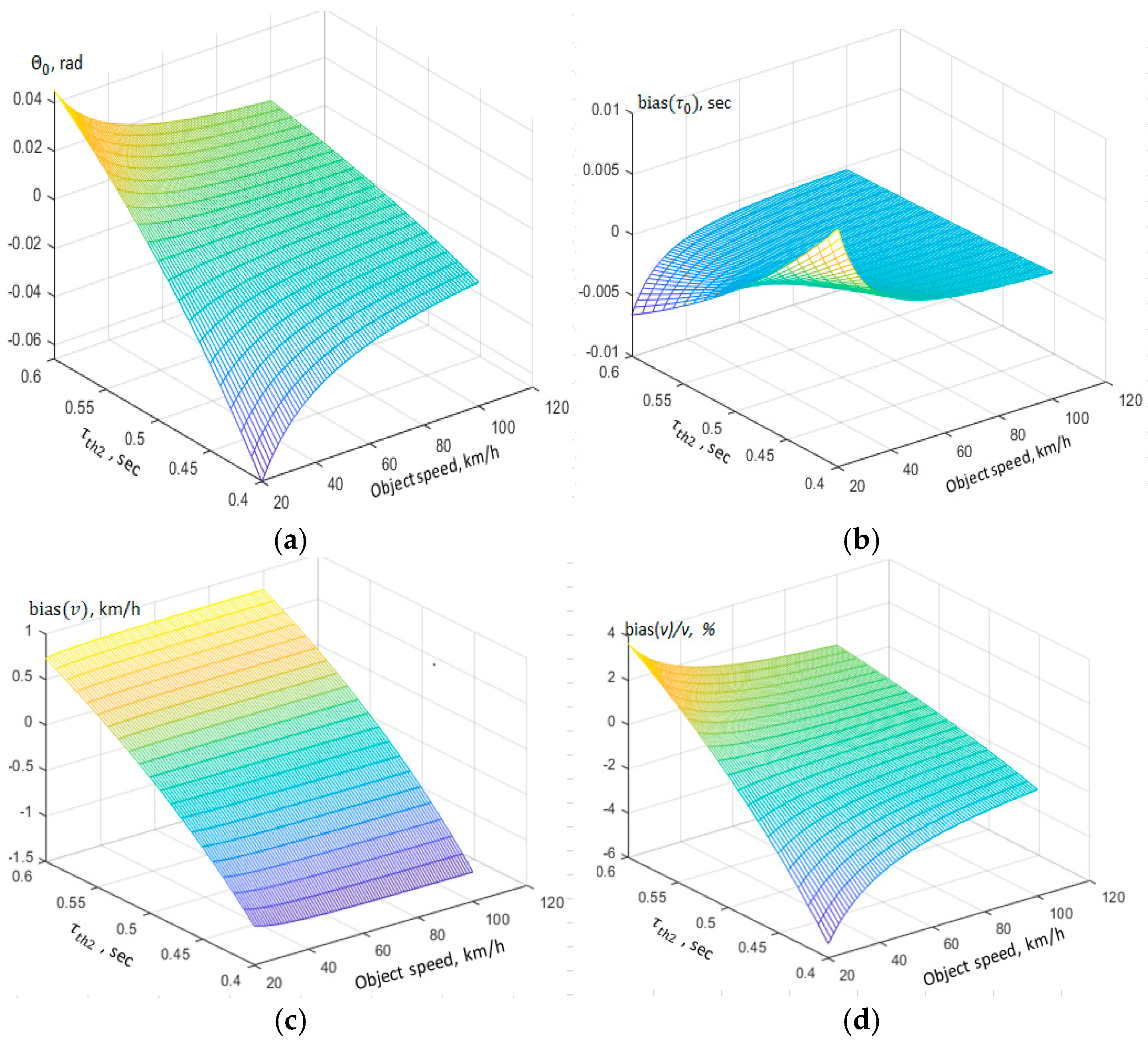
3.1. Numerical Results

This section presents numerical results for time period estimation (TPE) in vehicle speed measurement using pyroelectric infrared (PIR) sensors. This study evaluates two methods: cross-correlation function (CCF) and cross-correlation function with Hilbert transform (CCFHT). The focus is on how sensor response mismatch, noise levels, and signal bandwidth affect the estimation accuracy. The parameters used in this work are presented in

Table 2. Key parameters and their values for simulation.

Quantity, [Unit]	Value
$\mathrm{Focal} \mathrm{length} \mathrm{of} \mathrm{both} \mathrm{sensors} F_1=F_2$, [mm]	50.9
Sensing element width w, [mm]	3
Distance between two sensors’ axes d, [m]	1
Distance to object’s (vehicle’s) movement D, [m]	10
Length of the object L, [m]	4.5
$\mathrm{Electrical} \mathrm{time} \mathrm{constant} {\tau }_{e1 }$(first sensor), [s]	0.08
$\mathrm{Thermal} \mathrm{time} \mathrm{constant} {\tau }_{th1}$(first sensor), [s]	0.5
$\mathrm{Electrical} \mathrm{time} \mathrm{constant} {\tau }_{e2 }$(second sensor), [s]	0.08
$\mathrm{Thermal} \mathrm{time} \mathrm{constant} {\tau }_{th2 }$(second sensor), [s]	0.4 ÷ 0.6
Number of discrete frequency bins Nd	1024
Noise bandwidth B, [Hz]	10 ÷ 100
Signal-to-noise ratios SNR1 = SNR2	10

.

It should be noticed that, if the object is moving with the speed v at the distance D from the sensors, then the duration of the signal caused by the moving object to the sensor and the signal frequency are defined as:

$$T_0={\displaystyle \frac{D\ast \left(\frac{w}{F}\right)+L}{v}}$$

(57)

$$f_0={\displaystyle \frac{1}{T_0}}={\displaystyle \frac{v}{D\ast \left(\frac{w}{F}\right)+L}}$$

(58)

On the other hand, once the bias and the variance of time period estimation are found, from (1), the bias and uncertainty of speed measurement due to the bias and variance of the TPE are also defined:

$$bias \left(v\right)=-{\displaystyle \frac{v^2}{d}}·bias\left({\tau }_0\right)$$

(59)

$$u\left(v\right)={\displaystyle \frac{v^2}{d}}·u\left({\tau }_0\right)={\displaystyle \frac{v^2}{d}}·\sqrt{var\left({\tau }_0\right)}$$

(60)

The numerical results are in the following figures. Figure 4, Figure 5 and Figure 6, which illustrate the effects of thermal time constant mismatch and object speed on TDE performance. Particularly, Figure 4 presents the influence of thermal time constant mismatch on the bias and variance of time period estimation. When the second sensor has a longer or shorter response time compared with the first, asymmetric signal shapes are produced, leading to a phase shift between the signals. Figure 5 shows that, while both methods are influenced, CCFHT maintains more stable variance across varying levels of sensor mismatch. In addition, Figure 6 also presents the impact of bandwidth B on TDE variance and speed measurement uncertainty using CCF.

3.2. Experimental Validation

To validate the numerical results, a practical experiment was conducted using real traffic vehicles under field conditions. The measurement system employed two PIR sensor modules arranged in a linear configuration with a fixed spacing of 1 m, as shown in Figure 2a. The sensors were mounted at a height of approximately 1.5 m above ground level and aligned horizontally along the direction of vehicle movement (Figure 2b). The distance from the measurement system to the vehicle movement line varied from 5 to 15 m. The axes of the sensors were adjusted to maintain their parallelism, as shown in our previous works [27,28].

The analog output of each PIR sensor was digitized using a data acquisition module based on a microcontroller STM32L476RG [35] and sampled at 1024 Hz. A high-speed camera (200 fps) was simultaneously used as a reference measurement system, enabling the extraction of ground truth vehicle speeds by tracking vehicle position across successive video frames.

A total of about 100 random vehicles, including cars and motorcycles, with different traveling speeds ranging from 20 to 100 km/h, were recorded. The time period between the sampled output signals of the two PIR sensors was extracted using both the conventional cross-correlation function (CCF) and the Hilbert transform-enhanced cross-correlation function (CCFHT). The estimated vehicle speeds were then calculated using the known distance between the sensors’ axes and compared against the camera-based reference.

The experimental results, shown in Figure 7, indicate that both methods provide reasonable estimates of vehicle speed with absolute estimation errors under 5 km/h over the speed range of 20 to 100 km/h; particularly, that the deviation between the estimated vehicle speed and the reference speed remains within 5% across the specific speed range when using the conventional cross-correlation method (CCF), and within 3.5% when using the Hilbert transform-enhanced cross-correlation method (CCFHT).

4. Discussion

4.1. Effect of Sensor Mismatch on Bias and Variance of Time Period Estimation

One of the primary factors affecting time period estimation (TPE) accuracy is the mismatch in the sensor characteristics, particularly differences in thermal and electrical time constants between the two PIR sensors. This mismatch introduces a phase shift ${\Theta }_0$ between the sensor responses, leading to systematic errors in the TPE.

From Figure 4a, it is observed that the phase mismatch ${\Theta }_0$ increases as the thermal time constant ${\tau }_{th2}$ derives from ${\tau }_{th1}$. This leads to an increasing bias in TDE, as shown in Figure 4b, confirming that larger sensor response mismatches lead to greater bias in the estimated time period.

Equations (40) and (53) infer that bias decreases at higher signal frequencies, meaning that, at higher vehicle speeds, the impact of sensor mismatch on bias is reduced. This trend is supported by Figure 4c, where speed estimation bias decreases as vehicle speed increases, further confirming the inverse relationship between bias and signal frequency.

Variance analysis reveals key differences between CCF and CCFT in handling sensor mismatches. In addition, from Figure 5, it is observed that CCF variance increases rapidly with sensor mismatch, making it highly unstable, while CCFHT variance remains relative lower, confirming its robustness against sensor mismatches.

4.2. Impact of Bandwidth and Noise on Estimation Variance

The presence of noise in PIR sensor signals significantly affects TDE variance, making it an essential factor in performance evaluation. Mathematically, the variance behaviors using the two methods are given in Equations (38) and (51). These results confirm that CCF variance increases with B, whereas CCFHT remains stable across different bandwidth conditions. The numerical results also indicated that CCF-based TDE is highly sensitive to noise bandwidth. Specifically, as bandwidth increases, the variance in CCF-based time period estimation also increases significantly (Figure 6). This occurs because CCF variance scales directly with the noise bandwidth, making it unreliable for wideband signals.

This trend is evident in Figure 6, where it is seen that CCF variance increases dramatically at higher bandwidths. Meanwhile, CCFHT variance remains stable, confirming its ability to suppress noise-related uncertainty.

4.3. Implications for Practical Deployment

The findings of this study carry several implications for the practical deployment of TPE systems using low-cost PIR sensors. CCFHT demonstrates superior robustness to both sensor mismatch and environmental noise, making it a more viable option for real-world implementations where hardware constraints and variability are common. The mathematical framework developed in this study enables the quantitative prediction of estimation performance under different conditions. This allows system designers to assess expected error margins and choose parameters accordingly.

Despite the simplicity and low cost of the PIR-based system, the analytical and experimental results indicate that accurate speed estimation is achievable within typical traffic speed ranges (20–100 km/h), with mean estimation errors below 3.5% when using CCFHT.

While this paper focuses on two correlation-based techniques, it is important to note that other TPE methods have been proposed in the literature. For instance, generalized cross-correlation (GCC) [13] incorporates frequency domain weighting to improve delay detection in multipath or noisy environments, while wavelet-based approaches [22,36] leverage time–frequency analysis to handle non-stationary signals. Though potentially more accurate, these methods often demand greater computational resources, making them less suitable for embedded or low-power platforms such as those built around PIR sensors.

Future work may consider integrating lightweight machine learning models [37] to further improve performance, or multi-sensor fusion with complementary sensors (e.g., accelerometers, ultrasonic, or light sensors) to increase robustness under complex traffic and environmental conditions.

5. Conclusions

This study evaluated time period estimation (TDE) methods using pyroelectric infrared (PIR) sensors to determine vehicle speed in intelligent transportation systems (ITSs) based on a mathematical framework. The analysis focused on two correlation-based techniques: the conventional cross-correlation function (CCF) and an enhanced version using the Hilbert transform (CCFHT). A unified analytical framework was developed to derive bias and variance expressions for both methods under practical conditions involving sensor mismatch and noise. Numerical simulations demonstrated that, although both estimators yielded unbiased results in ideal conditions, sensor mismatch and bandwidth limitations significantly affected the performance of CCF. In contrast, CCFHT maintained a lower estimation variance across varying mismatch levels and noise bandwidths, confirming its robustness and stability. Experimental results further validated the findings, showing that CCFHT consistently achieved speed estimation errors below 3.5% in real-world vehicle traffic scenarios, compared with 5% for CCF. These results highlight the potential of low-cost PIR sensors, combined with carefully selected signal processing techniques such as CCFHT, for reliable and energy-efficient vehicle speed monitoring in intelligent transportation systems (ITSs). Moreover, integrating other types of sensors and applying more advanced signal processing algorithms are essential to further improve the system’s performance, representing a critical development trend for ITSs.

References

1. Papageorgiou, M.; Diakaki, C.; Dinopoulou, V.; Kotsialos, A.; Wang, Y. Review of road traffic control strategies. Proc. IEEE 2003, 91, 2043–2067. [Google Scholar] [CrossRef]
2. Zhang, C.; Shen, S.; Huang, H.; Wang, L. Estimation of the Vehicle Speed Using Cross-Correlation Algorithms and MEMS Wireless Sensors. Sensors 2021, 21, 1721. [Google Scholar] [CrossRef] [PubMed]
3. Duda, K.; Marszalek, Z. Vehicle speed determination with inductive-loop technology and fast and accurate fractional time delay estimation by DFT. Metrol. Meas. Syst. 2024, 31, 781–796. [Google Scholar] [CrossRef]
4. Kaskonas, P.; Meskuotiene, A. Vehicle Speed Meters Validation and Verification System. Elektron. Elektrotech. 2012, 3, 95–98. [Google Scholar] [CrossRef]
5. O’Dwyer, A. Time Delay Estimation in Signal Processing Applications: An Overview. In Proceedings of IT&T Conference; Waterford Institute of Technology: Waterford, Ireland, 2002. [Google Scholar]
6. Hing, C.S. Time Delay Estimation: Applications and Algorithms. 2015. Available online: https://sigport.org/sites/default/files/Time_Delay_Estimation.pdf (accessed on 25 April 2025).
7. Luz, E.Y.; Mimbela, A. Summary of Vehicle Detection and Surveillance Technologies Used in Intelligent Transportation Systems; Technical Report; The Vehicle Detector Clearinghouse, Southwest Technology Development Institute (SWTDI) at New Mexico State University: Las Cruces, NM, USA, 2007. [Google Scholar]
8. Arora, A.; Dutta, P.; Bapat, S.; Kulathumani, V.; Zhang, H.; Naik, V.; Mittal, V.; Cao, H.; Demirbas, M.; Gouda, M.; et al. A line in the sand: A wireless sensor network for target detection, classification, and tracking. Comput. Networks 2004, 46, 605–634. [Google Scholar] [CrossRef]
9. Garcia, F.; Cerri, P.; Broggi, A.; Armingol, J.M.; de la Escalera, A. Vehicle detection based on laser radar. In Computer Aided Systems Theory—EUROCAST 2009; Springer: Berlin/Heidelberg, Germany, 2009; pp. 391–397. [Google Scholar]
10. Michalopoulos, P.G. Vehicle detection video through image processing: The Autoscope system. IEEE Trans. Veh. Technol. 1991, 40, 21–29. [Google Scholar] [CrossRef]
11. Tarik, M.H.; Ahsen, M.B.; Tarek, N.S.; Samir, A.A. Infrared Pyroelectric Sensor for Detection of Vehicular Traffic Using Digital Signal Processing Techniques. IEEE Trans. Veh. Technol. 1995, 44, 683–689. [Google Scholar]
12. Odat, E.; Shamma, J.S.; Claudel, C. Vehicle Classification and Speed Estimation Using Combined Passive Infrared/Ultrasonic Sensors. IEEE Trans. Intel. Transp. Syst. 2018, 19, 1593–1606. [Google Scholar] [CrossRef]
13. Knapp, C.; Carter, G. The generalized correlation method for estimation of time delay. IEEE Trans. Acoust. Speech Signal Process. 1976, 24, 320–327. [Google Scholar] [CrossRef]
14. Carter, G.C. Coherence and time delay estimation. Proc. IEEE 1987, 75, 236–255. [Google Scholar] [CrossRef]
15. Brandstein, M.; Ward, D. Microphone Arrays: Signal Processing Techniques and Applications; Springer: Berlin/Heidelberg, Germany, 2001. [Google Scholar]
16. Blok, E. Classification and evaluation of discrete subsample time delay estimation algorithms. In Proceedings of the 14th International Conference on Microwaves, Radar and Wireless Communications MIKON-2002, Gdansk, Poland, 20–22 May 2002. [Google Scholar]
17. Bendat, J.S.; Piersol, A.G. Random Data—Analysis and Measurement Procedures, 4th ed.; Wiley: New York, NY, USA, 2010. [Google Scholar]
18. Costa-Júnior, J.F.; Cortela, G.A.; Maggi, L.E.; Rocha, T.F.; Pereira, W.C.; Costa-Felix, R.P.; Alvarenga, A.V. Measuring uncertainty of ultrasonic longitudinal phase velocity estimation using different time-delay estimation methods based on cross-correlation: Computational simulation and experiments. Measurement 2018, 122, 45–56. [Google Scholar] [CrossRef]
19. Lampropoulos, G.; Chan, Y. Time delay estimation with nonstationary signals. In Proceedings of the ICASSP ’86. IEEE International Conference on Acoustics, Speech, and Signal Processing, Tokyo, Japan, 7–11 April 1986. [Google Scholar]
20. Pang, Z.; Wang, G.; Wang, B.; Wang, L. Comparison between Time Shifting Deviation and Cross-correlation Methods. J. Light. Technol. 2022, 40, 3003–3009. [Google Scholar] [CrossRef]
21. Tamim, S.M.; Ghani, F. Hilbert transform of FFT pruned cross correlation function for optimization in time delay estimation. In Proceedings of the IEEE 9th Malaysia International Conference on Communications (MICC), Kuala Lumpur, Malaysia, 15–17 December 2009. [Google Scholar]
22. Osman, A.B.; Ovinis, M.; Hashim, F.M.; Mohammed, K.; Osei, H. Time Delay Estimation Using Continuous Wavelet Transform Coefficients. Adv. Sci. Lett. 2017, 23, 1299–1303. [Google Scholar] [CrossRef]
23. Hanus, R. Time delay estimation of random signals using cross-correlation with Hilbert Transform. Measurement 2019, 146, 792–799. [Google Scholar] [CrossRef]
24. Donovan, B.; Li, Y.; Stern, R.; Jiang, J.; Claudel, C.; Work, D. Vehicle detection and speed estimation with PIR sensors. In Proceedings of the 14th International Conference on Information Processing in Sensor Networks, Seattle, WT, USA, 13–16 April 2015; pp. 370–371. [Google Scholar]
25. Van Quang, V.; Thang, V.T. A novel system for measuring vehicle speed via analog signals of pyroelectric infrared sensors. Int. J. Mod. Phys. B 2021, 35, 2140028. [Google Scholar] [CrossRef]
26. So, H.C.; Chan, Y.T.; Ho, K.C.; Chen, Y. Simple Formulas for Bias and Mean Square Error Computation. IEEE Signal Process. Mag. 2013, 30, 162–165. [Google Scholar] [CrossRef]
27. Thang, V.T.; Van Quang, V.; Bui, N.T. A Setup for Measuring the Centering Error of a Dual-Element Pyroelectric Infrared Sensor Module. Sensors 2021, 21, 6684. [Google Scholar] [CrossRef]
28. Van Quang, V.; Thang, V.T. Measurement uncertainty analysis of centering error of pyroelectric infrared sensor module. Infrared Phys. Technol. 2024, 137, 105124. [Google Scholar] [CrossRef]
29. Yun, J.; Song, M.-H. Detecting Direction of Movement Using Pyroelectric Infrared Sensors. IEEE Sens. J. 2014, 14, 1482–1489. [Google Scholar] [CrossRef]
30. Bodhibrata, M.; Seshan, S.; Subrat, K. Modeling the Analog Response of Passive Infrared Sensor. Sensors Sens. Actuators A Phys. 2018, 279, 65–74. [Google Scholar]
31. Whatmore, R.W. Pyroelectric Devices and Materials. Rep. Prog. Phys. 1999, 49, 1335. [Google Scholar] [CrossRef]
32. Pillai, S. Unnikrishna. In Probability, Random Variables, and Stochastic Processes; McGraw-Hill: New York, NY, USA, 2002. [Google Scholar]
33. Kay Steven, M. Fundamentals of Statistical Signal Processing: Estimation Theory; Prentice-Hall, Inc.: Hoboken, NJ, USA, 1993. [Google Scholar]
34. Faerman, V.; Avramchuk, V.; Voevodin, K.; Sidorov, I.; Kostyuchenko, E. Study of Generalized Phase Spectrum Time Delay Estimation Method for Source Positioning in Small Room Acoustic Environment. Sensors 2022, 22, 965. [Google Scholar] [CrossRef] [PubMed]
35. Datasheet of Microcontrollers STM32L476xx. STMicroelectronics. Available online: https://www.st.com/resource/en/datasheet/stm32l476je.pdf (accessed on 25 April 2025).
36. Sharkova, S.B.; Faerman, V.A. Wavelet transform-based cross-correlation in the time-delay estimation applications. J. Phys. Conf. Ser. 2021, 2142. [Google Scholar] [CrossRef]
37. Shaltaf, S. Neural-Network-Based Time-Delay Estimation. EURASIP J. Adv. Signal Process. 2004, 3, 378–385. [Google Scholar] [CrossRef]
Figure 1. Graphical illustration of a practical objective function.
Applsci 15 06255 g001
Figure 2. Views of the speed measurement systems using two PIR sensors (a); and illustration of its working principle (b).
Applsci 15 06255 g002aApplsci 15 06255 g002b
Figure 3. PIR sensors perform as linear systems.
Applsci 15 06255 g003
Figure 4. Impact of various time constant ( τ t h 2 ) and object speed on: (a) argument Θ 0 ; (b) time period estimation bias; (c) speed measurement bias; (d) relative speed measurement bias.
Applsci 15 06255 g004
Figure 5. Impact of various time constant ( τ t h 2 ) and object speed on estimation variances, in case B = 100 Hz: (a) variance of time period estimation using CCF; (b) variance of time period estimation using CCFHT; (c) uncertainty of speed measurement using CCF; (d) uncertainty of speed measurement using CCFHT; (e) relative difference between uncertainty of speed measurement using CCF and CCFHT.
Applsci 15 06255 g005
Figure 6. Impact of bandwidth on TDE (a) variance and speed measurement (b) uncertainty using CCF.
Applsci 15 06255 g006
Figure 7. Comparison between reference vehicle speeds (obtained from video) and estimated speeds using the CCF and CCFHT methods (a); and estimation errors of vehicle speeds using the CCF and CCFHT methods under real conditions (b).
Applsci 15 06255 g007