Time Series Anomaly Detection Using Signal Processing and Deep Learning

Abstract

In this paper, we propose a two-step approach for time series anomaly detection that combines signal processing techniques with deep learning methods. In the first step, we apply a bandpass filter to the time series data to reduce noise and highlight relevant frequency components, which enhances the signals in them. In the second step, we utilize a Functional Neural Network Autoencoder for anomaly detection, leveraging its ability to capture non-linear temporal relationships in the data. By learning a compact latent representation and remapping the filtered time series, the Autoencoder effectively identifies deviations from normal patterns, allowing us to detect anomalies. Our experiments on several benchmark datasets demonstrate that bandpass filtering consistently improves the performance of deep learning methods, including the Functional Neural Network Autoencoder, by refining the input data. Our proposed approach achieves superior performance of up to 20% in detecting anomalies, particularly in a time series with intricate structures, highlighting its potential for practical applications in multiple domains.

1. Introduction

Anomaly detection in time series data is a critical task in numerous real-world applications, ranging from Industrial Monitoring and Predictive Maintenance to Fraud Detection and Healthcare Analytics [1,2]. Anomalies often signify critical events that differ greatly from expected behavior, such as equipment failures, fraudulent activities, or unusual patient conditions, and therefore require immediate attention [3,4]. However, detecting such anomalies in time series data remains a challenging task due to the presence of noise, seasonality, and non-stationary characteristics inherent in real-world signals recorded over time.

Effective anomaly detection methods for time series data require training machine learning models that can capture the temporal dynamics as well as the contextual patterns of normal behavior using either supervised or unsupervised learning approaches. Supervised methods [5,6] rely on labeled datasets that distinguish normal from anomalous data; however, labeled anomalies are not common, especially for rare events, limiting the applicability of such methods. On the other hand, unsupervised learning focuses on training models solely on normal data, which allows it to detect anomalies as deviations from learned patterns. This makes unsupervised methods particularly valuable for anomaly detection, where labeled anomalies are either rare or expensive to obtain while normal data are readily available.

Traditional time series processing methods, such as statistical models like the ARIMA (Auto-Regressive Integrated Moving Average) [7] or signal processing techniques [8], have shown success in specific settings but often fail to adapt to complex, high-dimensional time series data. With the rise of deep learning, more sophisticated models have been developed that can automatically learn patterns in time series data without the need for extensive feature engineering. Models like Autoencoders, which is an unsupervised approach, with layers of traditional neural networks, Recurrent Neural Networks (RNNs), Transformers, and Convolutional Neural Networks (CNNs) are commonly used for time series anomaly detection [9,10,11]. Autoencoders have shown they can learn compact representations of normal time series data, from which they are able to remap back to the original time series and flag deviations from these learned patterns. Long Short-Term Memory (LSTM) networks, a type of RNN, are frequently used for time series analysis due to their ability to capture long-term temporal dependencies, making them particularly effective for detecting anomalies in such kind of data [12].

Recent research in deep learning has highlighted the effectiveness of more advanced architectures such as Transformers [13] and Graph Neural Networks (GNNs) [14] for time series anomaly detection. Transformers, with their self-attention mechanisms, are particularly capable of capturing global dependencies in long sequences, making them suitable for multivariate time series anomaly detection where time series feature relationships are critical. Graph Neural Networks explicitly model the relational structure between different time series features, enabling a better understanding of spatial and temporal dependencies in complex systems. As mentioned in [15,16,17], these deep learning approaches represent a significant leap forward in the ability to detect anomalies in real-world time series data.

Another promising deep learning approach for time series analysis is the Functional Neural Network (FNN), designed to handle time series data by treating them as continuous functions rather than discrete data points [18]. This allows FNNs to capture both local and global temporal patterns, making them well suited for dealing with intricate, high-dimensional time series data. By learning non-linear relationships while preserving the temporal structure, FNNs offer a robust method for analyzing time series data. Building on this, Bi-Functional Autoencoders (BFAEs) [19] extend the FNN framework to enable dimensionality reduction using an Autoencoder architecture. The BFAE learns a compact representation of the time series, achieving efficient data compression. However, the BFAE has not been tested for anomaly detection tasks. In this paper, we explore its potential for anomaly detection, as its ability to compress and reconstruct functional data makes it a promising approach for identifying anomalous patterns in a time series.

Despite their success, machine learning and deep learning models are often sensitive to noise and irrelevant patterns present in time series data, which can lead to reduced accuracy in detecting anomalies. To address this, preprocessing techniques, such as filtering, have been introduced to clean the data before applying models [20,21] for time series tasks. Bandpass, bilateral, and other filtering approaches have shown promise in isolating specific frequency ranges that contain the most relevant information while removing noise, improving the performance of downstream anomaly detection [8].

In this paper, we propose a novel two-step approach that combines bandpass filtering with deep learning-based Autoencoders for anomaly detection in time series data. The data processing step uses a bandpass filter to help remove noise and irrelevant frequency components, allowing the deep learning models to focus on capturing the essential dynamics of the time series. We leverage the Functional Neural Network Autoencoder, which is particularly adept at handling complex temporal patterns, to detect anomalies. We perform extensive experiments on various benchmark datasets to demonstrate the effectiveness of our method in improving the accuracy of anomaly detection compared to other approaches.

This paper is structured as follows: Section 2 provides a comprehensive review of the literature relevant to time series anomaly detection. Section 3 shares the proposed methodology and key concepts used in this work. Section 4 dives into the results across different datasets along with discussing key observations. Finally, Section 5 offers conclusions and suggests avenues for future research.

2. Literature Review

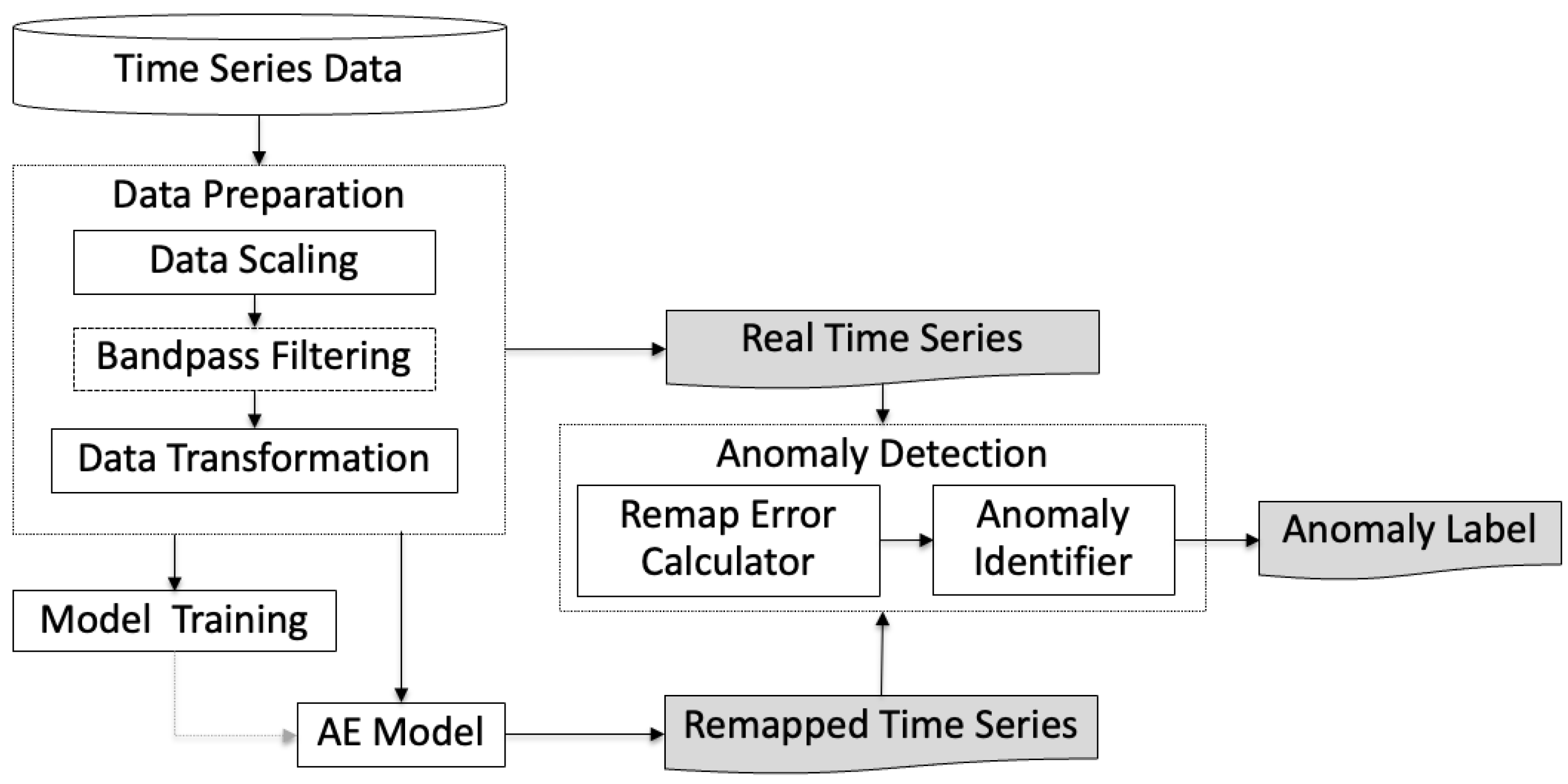
Time series anomaly detection has been an area of interest recently due to its importance in various applications. Traditional approaches, such as statistical methods, rely on building models that assume particular properties of the time series data. For example, the ARIMA and its variants are commonly used for anomaly detection by modeling the temporal behavior of the data and identifying deviations from predicted trends [22,23]. However, these methods are limited in handling complex and non-stationary time series data.

More recently, machine learning approaches have gained prominence for anomaly detection in time series. Unsupervised methods, in particular, reconstruction-based approaches, where Autoencoder models are widely used to learn compressed representations of the input data from which the original data are remapped. Autoencoders [24] consist of an encoder, which maps the input data into a lower-dimensional latent space, and a decoder, which reconstructs the input from the latent representation. In the context of time series anomaly detection, Autoencoders are trained on normal data to learn the regular patterns of the time series. During inference, data points that result in high reconstruction errors are detected as anomalies. The performance of Autoencoders is highly dependent on the quality of the training data, and they might not learn meaningful latent presentations if the data have a lot of noise or is sparse. Variants of Autoencoders, such as Denoising Autoencoders and Variational Autoencoders (VAEs), have been introduced to improve robustness and generalization. VAEs [25] are explicitly trained to model a probabilistic distribution of the input data, but it is challenging to appropriately learn the underlying data distribution or long-term dependencies in time series data without further prior knowledge incorporation [26]. Denoising Autoencoders [27] learn robust latent representations by reconstructing the original input data from a noisy version of the input. Here, prior assumptions about the level and type of noise are necessary to ensure modeling success. Different deep learning network architecture variants, such as temporal convolutional Autoencoders [28] and LSTM-based Autoencoders [29,30] have been explored to better capture the temporal dependencies in time series data during reconstruction. These models either assume a particular structure in the time series data or have restricting network flexibility that limits the performance.

Other traditional approaches for time series analysis leverage signal processing techniques to decompose time series signals into time and frequency components. Fourier Transform (FFT) and Short-Time Fourier Transform (STFT) enable frequency-domain analysis [31] to identify anomalies through irregularities in the spectral domain. Wavelet Transform (WT) [32] extends this by providing a multi-scale time–frequency representation to allow the localized detection of anomalies across different resolutions. Hybrid machine learning approaches can tackle both time and frequency features to address complex patterns in time series data and increase model performance. For example, time–frequency information derived from Wavelets can be combined with Convolutional Neural Networks (CNNs) to detect irregularities in the data [33,34]. Similarly, the network architectures of the LSTM and Squeeze and Excitation Network (SENet) were combined with an FFT-constructed frequency matrix to improve time series anomaly detection in [35]. Traditional Autoencoders may inadvertently reconstruct anomalies due to their ability to capture complex features in latent spaces. Dr. Yao et al. [36] proposed a novel approach to mitigate this by integrating Wavelet Transform into the Autoencoder architecture as a regularization mechanism.

Another way to look at time series data is through Functional Data Analysis (FDA) [37]. It provides powerful tools for time series anomaly detection by treating time series data as functions rather than discrete observations. Using basis expansion techniques, such as Fourier, Wavelet, or B-spline bases, FDA transforms a time series into a smooth, continuous representation. This enables the robust modeling of temporal information, reducing noise and highlighting deviations from normal behavior. Functional models have received a lot of success in different time series tasks [38,39]. Anomaly detection can be performed by fitting a functional model to a collection of a normal time series and measuring how new observations deviate from the expected functions. Recent approaches leverage functional Autoencoders [19,40], which combine FDA with deep learning. In these methods, time series data are encoded into a lower-dimensional latent space using functional transformations and are then reconstructed. Functional Autoencoders excel at capturing complex, non-linear dependencies in a time series and enable two-way dimensionality reduction in the feature as well as time domain. This dual nature allows efficient representation learning and remapping. Although functional Autoencoders have not yet been applied explicitly for anomaly detection, their ability to capture intricate patterns and temporal relations make them a promising and logical next step for advancing anomaly detection techniques.

Despite their success, Autoencoder models can be sensitive to noise and irrelevant features in the input time series, which can deteriorate their anomaly detection performance. On the other hand, signal processing cannot learn complex relations. This motivates the need to merge these two ideas. Preprocessing techniques, such as filtering, can improve the quality of the input data and increase modeling success. Different applications of time series filters can be found in the literature: smoothing (e.g., moving averages and the Gaussian filter), Wavelet Transform [30], Non-Linear Filtering [41], Bayesian [42], Fourier Transform (e.g., FFT), Kernel methods [43,44], Savitzky–Golay filter [45], or Decompositions (e.g., STL [46,47]). Bandpass filtering [31] is a signal processing technique that allows the retaining of frequency components within a specified range while removing those outside the range such as removing low-frequency trends or high-frequency noise. Bandpass filters are widely used in applications such as communication systems, biomedical signal processing, and vibration analysis to remove noise and isolate relevant frequency components to enhance signal quality [48,49].

While bandpass filtering has been used extensively in signal processing, its integration with machine learning models for time series anomaly detection has not been widely explored. Combining bandpass filtering with Autoencoder-based models provides an opportunity to leverage the strengths of both approaches: the noise reduction capabilities of filtering and the representation learning from Autoencoders.

3. Methodology

Figure 1 shows the overall workflow of our proposed method. First, the time series data are preprocessed with data scaling, bandpass filtering, and data transformation based on the neural network architecture of choice (data preparation step). Secondly, an Autoencoder model is trained using normal (non-anomalous) time series data (model training step), which can finally be leveraged to obtain remapped time series predictions to compute the remapping error. If the remapping error is larger than a threshold, an anomaly is detected.

3.1. Data Preparation

Data preparation is crucial for adjusting the time series data to make them digestible by the model. The first step involves applying data scaling, such as standardization, to ensure that the data have a mean of zero and a variance of one, which helps improve model performance and convergence. Additionally, data transformation is performed so that the data dimensions align with the chosen neural network architecture. Time series data are then segmented using non-overlapping sliding windows to obtain a set of time series samples [50]. The sliding window size needs to be chosen carefully, depending on the specific problem and the temporal resolution required for analysis.

The next key step is bandpass filtering. It is a signal processing technique that allows only a specific range of frequencies within a signal to pass through while removing components outside this range. As an additional preprocessing step in time series data analysis, it is particularly useful for improving signal quality by removing undesired noise or trends that may mask meaningful patterns. A bandpass filter is defined by two cutoff frequencies:

• Low cutoff frequency—removes components with frequencies below it (e.g., trends or baseline drift).
• High cutoff frequency—removes components with frequencies above it (e.g., random noise).

The signal components that fall within these two frequencies are preserved, allowing for the extraction of dominant periodicities or oscillations in the specified range. In practice, digital bandpass filters, such as Butterworth, Chebyshev, Elliptic, or finite impulse response (FIR) filters [51], are commonly employed to achieve smooth filtering with minimal distortion.

In the bandpass filtering step of our data preparation process, we use a Butterworth filter [44]. Generally, prior spectral analysis (e.g., using Fourier Transform or Power Spectral Density) helps determine the dominant frequency components to preserve. However, in the scope of this paper, we decide the low and high cutoff frequencies based on the overall length of the signal (i.e., the sliding window length) to focus on the intermediate frequency band where the core signal resides. Given that the sliding window size is chosen appropriately according to the problem at hand, we can use proportional lower and higher cutoff frequencies, e.g., cutting 10% on each side of the frequency spectrum. Since bandpass filtering emphasizes repeating patterns in the data, it can help the Autoencoder models to concentrate on learning important patterns from the data and therefore improve the accuracy and reliability of downstream analyses, such as feature extraction, anomaly detection, or predictive modeling.

3.2. Model Training

We train Autoencoder models with different neural network architectures to learn the normal state of the observed time series data. Autoencoder models are a type of artificial neural network architecture designed to learn an efficiently compressed representation (encoding) of input data by training them to reconstruct the input as closely as possible at the output layer after compression (decoding). Autoencoders consist of two primary components as seen in Figure 2:

• Encoder: Compresses the R dimensional input time series data $X\left(s\right)\in {\mathbb{R}}^R$, where $s\in S\subseteq \mathbf{R}$ and $S$ is a compact time interval, into a latent, lower-dimensional representation $Z\left(s^{\prime }\right)$ in the subsequent layers, where $Z\left(s^{\prime }\right)\in {\mathbb{R}}^{R^{\prime }}$, where $R^{\prime }<R$, and where $s^{\prime }\in S^{\prime }\subseteq \mathbf{S}$. This process aims to retain the most relevant features of the data.
• Decoder: Reconstructs the original input as $\widehat{X\left(s\right)}\in {\mathbb{R}}^R$ from the latent representation $Z\left(s^{\prime }\right)$.

This bottleneck architecture forces the network to learn a compressed yet informative representation of the input time series, making Autoencoders valuable for dimensionality reduction, anomaly detection, and feature learning.

We explore three different Autoencoder architectures by replacing the red neurons in Figure 2 with traditional fully connected neurons, LSTM cells, or functional neurons, as described below.

3.2.1. MLP

The Multi-Layer Perceptron (MLP) Autoencoder [24] is a specific architecture of Autoencoders that utilizes fully connected (dense) network layers in both the encoder and decoder networks. The architecture can be described as follows:

• Encoder: Input data x, where x is a vector stitched together over the time points and features, pass through multiple fully connected layers with traditional neurons. The output of the latent representation z is given as follows:

  $$z=\sigma (b+W{h}_{z-1}),$$

  where b and W are the bias and weight parameters, $h_{z-1}$ is the output of the previous layer, and $\sigma (·)$ is the activation function.
• Decoder: The decoder mirrors the encoder with fully connected layers, reconstructing the input from z:

  $$\widehat{x}=\sigma (b+W{h}_{l-1}),$$

  where $h_{l-1}$ is the output of the previous layer before the output and l denotes the total number of layers in the network.

In an MLP architecture, data flow through the dense layers without loops or recurrences. The encoder and decoder are normally constructed symmetrical.

3.2.2. LSTM

Long Short-Term Memory is a type of RNN, specifically designed to capture long-term dependencies in sequential data, making them ideal for catching normal patterns in time series data. Other traditional RNNs often struggle with learning patterns that are separated by many time steps, but LSTMs address this issue by incorporating memory cells and sophisticated gating mechanisms. LSTM units [52] are composed of hidden states at the current and previous time step (short-term memory), cell states at the current and previous time step (long-term memory), and the input vector at the current time step. They use a forget gate, an input gate, and an output gate to control what information is processed and saved in the short-term and long-term memory.

The LSTM Autoencoder [53] extends the Autoencoder framework to handle sequential data by incorporating LSTM units for both the encoder and decoder. The architecture can be described as follows:

• Encoder: Input data $x=\{x_1,x_2,\dots ,x_S\}$, where S is the sequence length and $x_t\in {\mathbb{R}}^R$ (t = 1, 2, …, S), are passed through the LSTM layers. The LSTM processes the sequence step by step, updating its hidden states $h_t$ and cell states $c_t$:

  $$o_t,(h_t,c_t)=\mathrm{LSTM}(x_t,h_{t-1},c_{t-1}).$$
  The final hidden and cell states $(h_S,c_S)$ serve as the latent representation Z that summarizes the entire multivariate input sequence into two compact representations with dimensions (num_layers, hidden_size).
• Decoder: The hidden and cell states of the latent representation Z are used to initialize the decoder LSTM layers with $h_0^{\prime }=h_S$ and $c_0^{\prime }=c_S$ together with a zero input tensor ${\widehat{x}}_0$. The decoder then generates a reconstructed sequence of hidden states $\widehat{o}=\{{\widehat{o}}_1,{\widehat{o}}_2,\dots ,{\widehat{o}}_S\}$ using

  $${\widehat{o}}_t,h_t^{\prime },c_t^{\prime }=\mathrm{LSTM}({\widehat{x}}_0,h_{t-1}^{\prime },c_{t-1}^{\prime }).$$

Finally, a fully connected layer is used to reconstruct $\widehat{o}$ back to the multivariate time series input $\widehat{x}$:

$$\widehat{x}=\sigma (b+W{\widehat{o}}_t).$$

LSTM Autoencoders efficiently capture temporal information in the data and the obtained latent representation captures patterns across the entire sequence in compressed form.

3.2.3. FNN

A Functional Neural Network [18,54] is composed of a series of interconnected functional (continuous) neurons that are designed to process functional (time series) data. The input layer of the network takes in functional data, and each continuous neuron in the continuous hidden layer performs a non-linear transformation on the input data or values coming in from the previous layer. The output layer of the network produces a functional output that can be used for prediction, forecasting, or classification.

Due to the success of the FNN and Bi-Functional Autoencoder (BFAE) [19] in time series data, we extend its application to anomaly detection. Here, the FNN Autoencoder is the BFAE, where the network architecture is similar to that of the traditional Autoencoder but each component is a function rather than a scaler value. This is possible because of functional neurons which are given as follows:

$$H_{\left(l\right)}^{\left(r\right)}\left(s\right)=\sigma \left(b_{\left(l\right)}^{\left(r\right)}\left(s\right)+\sum _{j=1}^J\int w_{\left(l\right)}^{(r,j)}(s,t)H_{(l-1)}^{(r,j)}\left(t\right)dt\right)$$

where l indicates the layer and $r,j$ are the neurons, $l=1,2,3,\dots ,L$, $\sigma (·)$ is a non-linear activation function, $b_{\left(l\right)}^{\left(r\right)}$ is the intercept function, and $w_{\left(l\right)}^{(r,j)}$ is the bi-variate parameter function for the rth continuous neuron in the lth hidden layer coming from the jth continuous neuron of the $(l-1)$th hidden layer.

Now, let us see how this network functions using the continuous neurons defined above:

• Encoder: The input layer that consists of time series data is transformed into a latent representation at an intermediate continuous hidden layer, denoted as the $l^{\prime }\mathrm{th}$ layer. This constitutes the encoder part of the FNN Autoencoder architecture, referred to by the functional encoder. The reduced-dimensional representation of the input in the $l^{\prime }\mathrm{th}$ continuous hidden layer is given as follows:

  $${\mathbf{Z}}^{\left(r^{\prime }\right)}\left(s\right)=H_{\left(l^{\prime }\right)}^{\left(r^{\prime }\right)}\left(s^{\prime }\right),$$

  where $r^{\prime }=1,2,\dots ,R^{\prime }$ and $R^{\prime }<R$. Here, the function ${\mathbf{Z}}^{\left(r^{\prime }\right)}$ is observed at $S^{\prime }\le S$ time points.
• Decoder: From this latent representation, the network works toward getting to the output layer, reconstructing the functional input values through continuous neurons in subsequent hidden layers. This constitutes the decoder part of the network, referred to as the functional decoder. The reconstructed values of the input in the output layer are given as follows:

  $$\widehat{X^{\left(r\right)}\left(s\right)}=H_{\left(L\right)}^{\left(r\right)}\left(s\right).$$

In summary, the functional encoder maps the input from an R-dimensional functional space to an $R^{\prime }$-dimensional functional space, and the functional decoder reconstructs the input by mapping back from the $R^{\prime }$-dimensional functional space to the original R-dimensional functional space. The latent representation ${\mathbf{Z}}^{\left(r^{\prime }\right)}\left(s^{\prime }\right)$ offers considerable flexibility, allowing the number of functional features $R^{\prime }$ and the number of observed time points $S^{\prime }$ to be adjusted according to the specific task requirements.

Among these models, MLP is the least computationally expensive due to its simple feedforward structure. LSTMs are more resource intensive, as they maintain hidden states across time steps, increasing training time. FNNs incur the highest computational cost due to their functional representation, but their expressiveness often allows for better performance even with shallower networks.

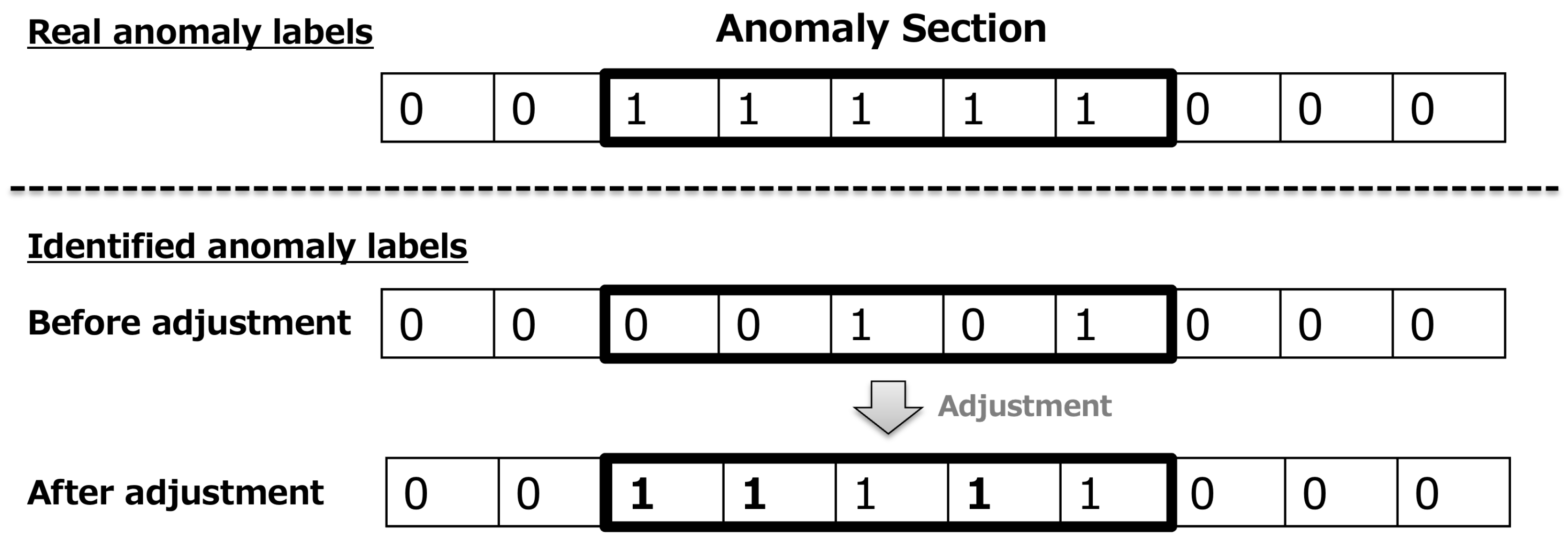
3.3. Anomaly Detection

We can leverage the trained Autoencoder models to compress newly observed time series data (encoding) and remap them into their original state (decoding). The remapped data can then be compared to the original input to calculate the difference as a remapping error. Here, we use the Mean Absolute Error (MAE) to calculate the remapping error for each sample. The MAE is given by Equation (1) for R multivariate time series features:

$$\mathrm{MAE}={\displaystyle \frac{1}{R}}\sum _{i=1}^R\int \left|\left(X_r\left(s\right)-\widehat{X_r\left(s\right)}\right)\right|dt.$$

(1)

In the second step, we want to identify each time step of the evaluation data as normal or an anomaly based on the remap error and a threshold. We hold out part of the model training data to validate the remap error range under a normal data setting and establish an anomaly threshold used in testing. In the proposed approach, the anomaly threshold is calculated based on the kth percentile of the error range. In our experiment, the 99th percentile is set as the cutoff, and the top 1% of the validation errors is set as the anomaly threshold. Using this threshold, we can identify the anomalies at each time step t.

Recently, it has become more common to use an adjustment strategy for partially detected anomaly sequences, as mentioned in [50,55,56]. The adjustment strategy works as a post-processing step that considers all time points in a certain successive abnormal segment as defects if the anomaly detection method successfully detects at least one time point of this segment. This strategy is based on the observation that an abnormal time point will cause an alert, which then draws attention to the whole segment. Therefore, in real-world applications, all anomalies in this abnormal segment would be correctly detected. An example of label adjustment is shown in Figure 3. Of the 10 observed time steps in this example, 5 consecutive time steps are anomalies. Initially, only two anomalous time steps are detected, but with the adjustment strategy, all five anomalous time steps are considered to be correctly identified.

4. Experiment and Results

In this paper, we experiment by adding a bandpass filtering step during the data preparation stage and then use Autoencoders with three neural network architectures (MLP, LSTM, and FNN) to see how the additional bandpass filtering step affects the performance for anomaly detection.

4.1. Real-World Datasets

We explore several real-world datasets as shown in

Table 1. Benchmark dataset information.

Dataset	# of Training Data	# of Test Data	Dimensions	Anomaly %
MSL [57]	58,317	73,729	55	10.5
SMAP [57]	135,183	427,617	25	12.8
SMD [56]	58,317	73,729	38	10.72
PSM [58]	132,481	87,841	25	27.8
SWAN [59]	60,000	60,000	38	32.6
SWAT [60]	99,000	89,984	26	12.2
WADI [61]	1,048,571	172,801	123	5.99

that have been used previously for time series anomaly detection tasks in the literature.

MSL and SMAP: Both MSL (Mars Science Laboratory rover) and SMAP (Soil Moisture Active Passive satellite) are public datasets from [57] with 55 and 25 dimensions, respectively, which contain the telemetry anomaly data derived from the Incident Surprise Anomaly (ISA) reports of spacecraft monitoring systems. In these multivariate datasets, most features only have binary values.

SMD: The Server Machine Dataset [56] was collected from a large Internet company with 38 dimensions (5 weeks of data total). We used 37 columns, eliminating 1 column without any value change.

PSM: The Pooled Server Metrics [58] dataset was collected internally from multiple application server nodes at eBay, and the dataset has 26 dimensions. SWAN: SWAN is a multivariate time series dataset with 38 features, and it contains solar photospheric vector magnetograms in the Spaceweather HMI Active Region Patch (SHARP) series [59,62].

SWaT: The Secure Water Treatment [60] is time series data from a modern industrial control system for security research and training that have 51 sensors under continuous operations. The data were collected over 11 days, and during the last 4 days, 36 attacks were launched with different intents and durations. After data cleaning, we used 41 columns, removing columns without value change and columns that have been recommended to be removed in [3].

WADI: The 14-day-long time series data from a water distribution system is presented in [61]. This testbed was used to analyze the security of water distribution networks and the effects of potential cyber and physical attacks. The dataset originally had 130 columns, but for our experiments, we reduced the dataset to 52 columns after eliminating highly correlated columns and columns without value changes.

Each benchmark dataset was pre-split into training and test data, where the training data were assumed to only have normal samples while the test data contained a mix of normal and abnormal samples. In our experimental setup, 20% of the training data were set aside for validation and a window size of 100 was used for all datasets, as recommended in [9]. We used a bandpass filter cutoff frequency of 5–45 Hz (based on the Nyquist frequency). The model’s hyperparameters were tuned using the validation data, which were also utilized to determine the anomaly detection threshold. This approach ensured that the model was optimized and calibrated before being evaluated on the test data. The experiments were performed on an 8-core M2 CPU, where the hyperparameter search for the number of layers (3, 5, 7), neurons (5, 10, 25, 50), activation functions (ReLU, Tanh, Linear), and others were kept in a similar range in the bottleneck network across the architectures (MLP, LSTM, and FNN) to ensure a fair comparison. We focused on matching the total number of trainable parameters so that each model had a similar capacity.

We evaluate our proposed anomaly detection approach (FNN) on seven real-world datasets, comparing it with two other neural network types (MLP and LSTM) and assessing the performance under both bandpass (BP) and No-bandpass (No BP) filtering settings.

Table 2. F1 score results comparing different methods.

Dataset	MLP (No BP)	MLP (BP)	LSTM (No BP)	LSTM (BP)	FNN (No BP)	FNN (BP)
MSL	0.871	0.863	0.886	0.863	0.849	0.846
SMAP	0.700	0.706	0.699	0.706	0.698	0.706
SMD	0.709	0.758	0.765	0.789	0.792	0.816
PSM	0.936	0.977	0.962	0.980	0.945	0.987
SWAN	0.791	0.795	0.789	0.793	0.801	0.819
SWAT	0.755	0.901	0.821	0.910	0.878	0.927
WADI	0.797	0.799	0.826	0.875	0.838	0.893

and

Table 3. AUC results comparing different methods.

Dataset	MLP (No BP)	MLP (BP)	LSTM (No BP)	LSTM (BP)	FNN (No BP)	FNN (BP)
MSL	0.930	0.928	0.940	0.934	0.925	0.922
SMAP	0.850	0.855	0.852	0.857	0.848	0.849
SMD	0.840	0.852	0.875	0.875	0.893	0.904
PSM	0.956	0.977	0.978	0.987	0.981	0.995
SWAN	0.861	0.865	0.860	0.865	0.870	0.881
SWAT	0.837	0.949	0.892	0.958	0.931	0.962
WADI	0.890	0.895	0.915	0.944	0.925	0.958

show the F1 score and AUC score results for all methods over the seven datasets, respectively. The F1 score is a useful metric for classification tasks because it balances two critical performance metrics: precision and recall, which are often at odds due to imbalanced classes (normal and anomaly) in anomaly detection tasks. On the other hand, AUC measures the model’s ability to rank positive instances higher than negative ones across all possible thresholds. This reflects the overall discrimination capability of the model. Both scores are key performance metrics. We can see from the tables that, for the MSL and SMAP datasets, the FNN with bandpass filtering does not perform well. This is because both the FNN and BP assume that the time series is derived from a continuous function, which is not valid for these datasets, where binary features are the majority. In contrast, for the other datasets (SMD, PSM, SWAN, SWAT, and WADI), where the time series are scalar functions, bandpass filtering significantly improves the results for each method, increasing the F1 scores by 0.25–20% and the AUC scores by 1–15%. Among these five datasets, the FNN Autoencoder models consistently outperform the alternatives, demonstrating their robustness in handling a scalar time series with bandpass filtering.

We performed a Monte Carlo simulation to estimate the variability in the F1 and AUC scores for each dataset using the FNN (BP) model. This involved repeatedly resampling the test data and computing the metrics to assess their variance. The maximum observed standard deviation for the F1 score was approximately 0.018, while for the AUC, it was around 0.010. Using these values, we constructed 95% confidence intervals for the performance comparison. Our analysis shows that for the SMD, PSM, SWAT, and WADI datasets, the FNN (BP) model not only outperforms the alternatives but does so with statistical significance. In contrast, for the SWAN dataset, while FNN (BP) performs well, the improvements are not statistically significant. For the MSL and SMAP datasets, the results indicate no strong performance advantage across the different models since the differences fall within the confidence interval.

4.2. Discussion

The experimental results highlight that the FNN is particularly well suited for time series data that possess underlying signal structures. This strength is further enhanced through the use of bandpass filtering, which refines the input to focus on relevant frequency components, reducing noise. FNNs are designed to capture complex temporal relationships while preserving the continuous nature of time series data throughout the network, unlike traditional architectures that may ignore time or treat time steps independently. As demonstrated in the prior literature, this inherent ability to model time series data enables FNNs to consistently achieve superior performance across a variety of time series tasks. Moreover, the FNN Autoencoder not only learns a compact feature representation but also maintains the temporal continuity of the data in the latent space, leading to more effective anomaly detection. Given these properties, FNN Autoencoders exhibit strong results in detecting anomalies, particularly in datasets where the time series behavior is structured and continuous.

However, as with many deep learning methods, FNNs require a sufficient amount of data to train effectively and are computationally intensive compared to simpler models. This introduces a trade-off between model performance and resource requirements. Several steps can be taken to mitigate these limitations, such as employing dimensionality reduction techniques, more efficient network architectures, or transfer learning approaches where feasible.

5. Conclusions

We introduced a novel two-step approach for time series anomaly detection, combining bandpass filtering with deep learning methods, specifically Functional Neural Network-based Autoencoders. The application of a bandpass filter in the preprocessing stage was shown to significantly increase the performance of the deep learning models by isolating relevant frequency components and removing noise. Our proposed method consistently outperformed traditional approaches across several benchmark datasets, demonstrating its efficacy in detecting anomalies in complex time series data.

The integration of the bandpass filter with the FNN offers a robust framework for handling a diverse and complex time series, providing a practical solution for anomaly detection in real-world applications. Our findings suggest that the preprocessing step of bandpass filtering generally boosts the performance, making it a versatile enhancement technique for time series analysis.

We plan to extend this approach to handle more challenging types of time series data, such as an intermittent time series using smoothing, spatiotemporal data, where standard anomaly detection methods often struggle, along with exploring other preprocessing methods (different signal processing approaches, functional principal components, and basis expansion), and incorporate some explainable AI techniques. Another direction would be to reduce the model complexity and computation using classical approaches or basis expansion in FNNs. Additionally, exploring more recent methods like Transformers, CNNs, and in particular, Variational Autoencoders (VAE), as a replacement for the standard Autoencoder is a promising direction. A VAE would allow us to model the distribution of a normal time series more effectively, providing a probabilistic framework for anomaly detection. This would enhance the robustness of the detection process, especially in environments with high uncertainty or varying patterns. Furthermore, probabilistic models can help refine anomaly scores and reduce false positives, thus improving the overall reliability of the system.

References

1. Darban, Z.Z.; Webb, G.I.; Pan, S.; Aggarwal, C.C.; Salehi, M. Deep Learning for Time Series Anomaly Detection: A Survey. arXiv 2022, arXiv:2211.05244. [Google Scholar]
2. Kim, S.M.; Kim, Y.S. Enhancing Sound-Based Anomaly Detection Using Deep Denoising Autoencoder. IEEE Access 2024, 12, 84323–84332. [Google Scholar] [CrossRef]
3. Wang, C.; Wang, B.; Liu, H.; Qu, H. Anomaly Detection for Industrial Control System Based on Autoencoder Neural Network. Wirel. Commun. Mob. Comput. 2020, 2020, 8897926:1–8897926:10. [Google Scholar] [CrossRef]
4. Lee, X.Y.; Kumar, A.; Vidyaratne, L.; Rao, A.R.; Farahat, A.; Gupta, C. An ensemble of convolution-based methods for fault detection using vibration signals. In Proceedings of the 2023 IEEE International Conference on Prognostics and Health Management (ICPHM), Montreal, QC, Canada, 5–7 June 2023; pp. 172–179. [Google Scholar] [CrossRef]
5. Roy, S.S.; Chatterjee, S.; Roy, S.; Bamane, P.; Paramane, A.; Rao, U.M.; Nazir, M.T. Accurate Detection of Bearing Faults Using Difference Visibility Graph and Bi-Directional Long Short-Term Memory Network Classifier. IEEE Trans. Ind. Appl. 2022, 58, 4542–4551. [Google Scholar] [CrossRef]
6. Abdallah, M.; Joung, B.G.; Lee, W.J.; Mousoulis, C.; Sutherland, J.W.; Bagchi, S. Anomaly Detection and Inter-Sensor Transfer Learning on Smart Manufacturing Datasets. Sensors 2022, 23, 486. [Google Scholar] [CrossRef]
7. Kozitsin, V.O.; Katser, I.D.; Lakontsev, D. Online Forecasting and Anomaly Detection Based on the ARIMA Model. Appl. Sci. 2021, 11, 3194. [Google Scholar] [CrossRef]
8. Yang, Y.; Zhang, C.; Zhou, T.; Wen, Q.; Sun, L. DCdetector: Dual Attention Contrastive Representation Learning for Time Series Anomaly Detection. In Proceedings of the 29th ACM SIGKDD Conference on Knowledge Discovery and Data Mining, Long Beach, CA, USA, 6–10 August 2023. [Google Scholar]
9. Xu, J.; Wu, H.; Wang, J.; Long, M. Anomaly Transformer: Time Series Anomaly Detection with Association Discrepancy. arXiv 2021, arXiv:2110.02642. [Google Scholar]
10. Wagner, D.; Michels, T.; Schulz, F.C.F.; Nair, A.; Rudolph, M.R.; Kloft, M. TimeSeAD: Benchmarking Deep Multivariate Time-Series Anomaly Detection. Trans. Mach. Learn. Res. 2023, 2023. [Google Scholar]
11. Yin, C.; Zhang, S.; Wang, J.; Xiong, N.N. Anomaly Detection Based on Convolutional Recurrent Autoencoder for IoT Time Series. IEEE Trans. Syst. Man Cybern. Syst. 2022, 52, 112–122. [Google Scholar] [CrossRef]
12. Wei, Y.; Jang-Jaccard, J.; Xu, W.; Sabrina, F.; Çamtepe, S.A.; Boulic, M. LSTM-Autoencoder-Based Anomaly Detection for Indoor Air Quality Time-Series Data. IEEE Sens. J. 2022, 23, 3787–3800. [Google Scholar] [CrossRef]
13. Tuli, S.; Casale, G.; Jennings, N.R. TranAD: Deep Transformer Networks for Anomaly Detection in Multivariate Time Series Data. Proc. VLDB Endow. 2022, 15, 1201–1214. [Google Scholar] [CrossRef]
14. Jin, M.; Koh, H.Y.; Wen, Q.; Zambon, D.; Alippi, C.; Webb, G.I.; King, I.; Pan, S. A Survey on Graph Neural Networks for Time Series: Forecasting, Classification, Imputation, and Anomaly Detection. IEEE Trans. Pattern Anal. Mach. Intell. 2023, 46, 10466–10485. [Google Scholar] [CrossRef]
15. Yan, P.; Abdulkadir, A.; Luley, P.P.; Rosenthal, M.; Schatte, G.A.; Grewe, B.F.; Stadelmann, T. A Comprehensive Survey of Deep Transfer Learning for Anomaly Detection in Industrial Time Series: Methods, Applications, and Directions. IEEE Access 2023, 12, 3768–3789. [Google Scholar] [CrossRef]
16. Schmidl, S.; Wenig, P.; Papenbrock, T. Anomaly Detection in Time Series: A Comprehensive Evaluation. Proc. VLDB Endow. 2022, 15, 1779–1797. [Google Scholar] [CrossRef]
17. Kim, B.; Alawami, M.A.; Kim, E.; Oh, S.; Park, J.H.; Kim, H. A Comparative Study of Time Series Anomaly Detection Models for Industrial Control Systems. Sensors 2023, 23, 1310. [Google Scholar] [CrossRef]
18. Rao, A.R.; Reimherr, M.L. Nonlinear Functional Modeling Using Neural Networks. J. Comput. Graph. Stat. 2021, 32, 1248–1257. [Google Scholar] [CrossRef]
19. Rao, A.R.; Wang, H.; Gupta, C. Functional approach for Two Way Dimension Reduction in Time Series. In Proceedings of the 2022 IEEE International Conference on Big Data (Big Data), Osaka, Japan, 17–20 December 2022; pp. 1099–1106. [Google Scholar]
20. Zhang, C.; Zhou, T.; Wen, Q.; Sun, L. TFAD: A Decomposition Time Series Anomaly Detection Architecture with Time-Frequency Analysis. In Proceedings of the 31st ACM International Conference on Information & Knowledge Management, Atlanta, GA, USA, 17–21 October 2022. [Google Scholar]
21. Giovannelli, A.; Lippi, M.; Proietti, T. Band-Pass Filtering with High-Dimensional Time Series. SSRN Electron. J. 2023. [Google Scholar] [CrossRef]
22. Yaacob, A.H.; Tan, I.K.; Chien, S.F.; Tan, H.K. ARIMA Based Network Anomaly Detection. In Proceedings of the 2010 Second International Conference on Communication Software and Networks, Singapore, 26–28 February 2010; pp. 205–209. [Google Scholar] [CrossRef]
23. Pena, E.H.M.; de Assis, M.V.O.; Proença, M.L. Anomaly Detection Using Forecasting Methods ARIMA and HWDS. In Proceedings of the 2013 32nd International Conference of the Chilean Computer Science Society (SCCC), Temuco, Chile, 11–15 November 2013; pp. 63–66. [Google Scholar] [CrossRef]
24. Hinton, G.E.; Salakhutdinov, R.R. Reducing the dimensionality of data with neural networks. Science 2006, 313, 504–507. [Google Scholar] [CrossRef]
25. Kingma, D.P. Auto-encoding variational bayes. arXiv 2013, arXiv:1312.6114. [Google Scholar]
26. He, S.; Du, M.; Jiang, X.; Zhang, W.; Wang, C. VAEAT: Variational AutoeEncoder with adversarial training for multivariate time series anomaly detection. Inf. Sci. 2024, 676, 120852. [Google Scholar] [CrossRef]
27. Vincent, P.; Larochelle, H.; Bengio, Y.; Manzagol, P.A. Extracting and composing robust features with denoising autoencoders. In Proceedings of the 25th International Conference on Machine Learning (ICML ’08), Helsinki, Finland, 5–9 July 2008; pp. 1096–1103. [Google Scholar] [CrossRef]
28. Thill, M.; Konen, W.; Wang, H.; Bäck, T. Temporal convolutional autoencoder for unsupervised anomaly detection in time series. Appl. Soft Comput. 2021, 112, 107751. [Google Scholar] [CrossRef]
29. Malhotra, P.; Ramakrishnan, A.; Anand, G.; Vig, L.; Agarwal, P.; Shroff, G. LSTM-based encoder-decoder for multi-sensor anomaly detection. arXiv 2016, arXiv:1607.00148. [Google Scholar]
30. Kanarachos, S.; Christopoulos, S.R.G.; Chroneos, A.; Fitzpatrick, M.E. Detecting anomalies in time series data via a deep learning algorithm combining wavelets, neural networks and Hilbert transform. Expert Syst. Appl. 2017, 85, 292–304. [Google Scholar] [CrossRef]
31. Oppenheim, A.V.; Schafer, R.W. Discrete-Time Signal Processing, 3rd ed.; Pearson: London, UK, 2009. [Google Scholar]
32. Meyer, Y. Wavelets: Algorithms and Applications; SIAM: Philadelphia, PA, USA, 1993. [Google Scholar]
33. Golgowski, M.; Osowski, S. Anomaly detection in ECG using wavelet transformation. In Proceedings of the 2020 IEEE 21st International Conference on Computational Problems of Electrical Engineering (CPEE), Online Conference, Poland, 16–19 September 2020; pp. 1–4. [Google Scholar] [CrossRef]
34. Shang, L.; Zhang, Z.; Tang, F.; Cao, Q.; Pan, H.; Lin, Z. CNN-LSTM Hybrid Model to Promote Signal Processing of Ultrasonic Guided Lamb Waves for Damage Detection in Metallic Pipelines. Sensors 2023, 23, 7059. [Google Scholar] [CrossRef]
35. Lu, Y.X.; Jin, X.B.; Chen, J.; Liu, D.J.; Geng, G.G. F-SE-LSTM: A Time Series Anomaly Detection Method with Frequency Domain Information. arXiv 2024, arXiv:2412.02474. [Google Scholar]
36. Yao, Y.; Ma, J.; Ye, Y. Regularizing autoencoders with wavelet transform for sequence anomaly detection. Pattern Recognit. 2023, 134, 109084. [Google Scholar] [CrossRef]
37. Kokoszka, P.; Reimherr, M.L. Introduction to Functional Data Analysis; Chapman and Hall/CRC: New York, NY, USA, 2017. [Google Scholar]
38. Shi, L.; Cao, L.; Chen, Z.; Chen, B.; Zhao, Y. Nonlinear subspace clustering by functional link neural networks. Appl. Soft Comput. 2024, 167, 112303. [Google Scholar] [CrossRef]
39. Wang, Q.; Zheng, S.; Farahat, A.K.; Serita, S.; Gupta, C. Remaining Useful Life Estimation Using Functional Data Analysis. In Proceedings of the 2019 IEEE International Conference on Prognostics and Health Management (ICPHM), San Francisco, CA, USA, 17–20 June 2019; pp. 1–8. [Google Scholar]
40. Hsieh, T.Y.; Sun, Y.; Wang, S.; Honavar, V.G. Functional Autoencoders for Functional Data Representation Learning. In Proceedings of the SDM, Virtual Event, 29 April–1 May 2021. [Google Scholar]
41. Shi, L.; Shen, L.; Zakharov, Y.V.; de Lamare, R.C. Widely Linear Complex-Valued Spline-Based Algorithm for Nonlinear Filtering. In Proceedings of the 2023 31st European Signal Processing Conference (EUSIPCO), Helsinki, Finland, 4–8 September 2023; pp. 1908–1912. [Google Scholar]
42. Feng, C.; Tian, P. Time Series Anomaly Detection for Cyber-physical Systems via Neural System Identification and Bayesian Filtering. In Proceedings of the 27th ACM SIGKDD Conference on Knowledge Discovery & Data Mining, Virtual Event, Singapore, 14–18 August 2021. [Google Scholar]
43. Shi, L.; Lu, R.; Liu, Z.; Yin, J.; Chen, Y.; Wang, J.; Lu, L. An Improved Robust Kernel Adaptive Filtering Method for Time-Series Prediction. IEEE Sens. J. 2023, 23, 21463–21473. [Google Scholar] [CrossRef]
44. Shi, L.; Tan, J.; Wang, J.; Li, Q.; Lu, L.; Chen, B. Robust kernel adaptive filtering for nonlinear time series prediction. Signal Process. 2023, 210, 109090. [Google Scholar] [CrossRef]
45. Singh, R.K.; Sinha, V.S.P.; Joshi, P.K.; Kumar, M. Use of Savitzky-Golay Filters to Minimize Multi-temporal Data Anomaly in Land use Land cover mapping. Indian J. For. 2019, 42, 362–368. [Google Scholar]
46. Cleveland, R.B.; Cleveland, W.S.; McRae, J.E.; Terpenning, I. STL: A seasonal-trend decomposition. J. Off. Stat 1990, 6, 3–73. [Google Scholar]
47. Tan, J.; Li, Z.; Zhang, C.; Shi, L.; Jiang, Y. A multiscale time-series decomposition learning for crude oil price forecasting. Energy Econ. 2024, 136, 107733. [Google Scholar] [CrossRef]
48. Hou, S.; Liang, M.; Zhang, Y.; Li, C. Vibration signal demodulation and bearing fault detection: A clustering-based segmentation method. Proc. Inst. Mech. Eng. Part C J. Mech. Eng. Sci. 2014, 228, 1888–1899. [Google Scholar] [CrossRef]
49. Selamat, N.A.; Ali, S.H.M. A Novel Approach of Chewing Detection based on Temporalis Muscle Movement using Proximity Sensor for Diet Monitoring. In Proceedings of the 2020 IEEE-EMBS Conference on Biomedical Engineering and Sciences (IECBES), Langkawi Island, Malaysia, 1–3 March 2021; pp. 12–17. [Google Scholar]
50. Shen, L.; Li, Z.; Kwok, J. Timeseries anomaly detection using temporal hierarchical one-class network. Adv. Neural Inf. Process. Syst. 2020, 33, 13016–13026. [Google Scholar]
51. Podder, P.; Hasan, M.M.; Islam, M.R.; Sayeed, M. Design and Implementation of Butterworth, Chebyshev-I and Elliptic Filter for Speech Signal Analysis. arXiv 2020, arXiv:2002.03130. [Google Scholar] [CrossRef]
52. Hochreiter, S. Long Short-term Memory. In Neural Computation; MIT-Press: Cambridge, MA, USA, 1997. [Google Scholar]
53. Malhotra, P.; Vig, L.; Shroff, G.M.; Agarwal, P. Long Short Term Memory Networks for Anomaly Detection in Time Series. In Proceedings of the European Symposium on Artificial Neural Networks, Bruges, Belgium, 22–24 April 2015. [Google Scholar]
54. Rao, A.R.; Reimherr, M.L. Modern non-linear function-on-function regression. Stat. Comput. 2023, 33, 130. [Google Scholar] [CrossRef]
55. Xu, H.; Feng, Y.; Chen, J.; Wang, Z.; Qiao, H.; Chen, W.; Zhao, N.; Li, Z.; Bu, J.; Li, Z.; et al. Unsupervised Anomaly Detection via Variational Auto-Encoder for Seasonal KPIs in Web Applications. In Proceedings of the 2018 World Wide Web Conference on World Wide Web—WWW ’18, Lyon, France, 23–27 April 2018; ACM Press: New York, NY, USA, 2018; pp. 187–196. [Google Scholar] [CrossRef]
56. Su, Y.; Zhao, Y.; Niu, C.; Liu, R.; Sun, W.; Pei, D. Robust Anomaly Detection for Multivariate Time Series through Stochastic Recurrent Neural Network. In Proceedings of the 25th ACM SIGKDD International Conference on Knowledge Discovery & Data Mining, KDD ’19, Anchorage, AK, USA, 4–8 August 2019; pp. 2828–2837. [Google Scholar] [CrossRef]
57. Hundman, K.; Constantinou, V.; Laporte, C.; Colwell, I.; Söderström, T. Detecting Spacecraft Anomalies Using LSTMs and Nonparametric Dynamic Thresholding. In Proceedings of the 24th ACM SIGKDD International Conference on Knowledge Discovery & Data Mining, London, UK, 19–23 August 2018. [Google Scholar]
58. Abdulaal, A.; Liu, Z.; Lancewicki, T. Practical Approach to Asynchronous Multivariate Time Series Anomaly Detection and Localization. In Proceedings of the 27th ACM SIGKDD Conference on Knowledge Discovery & Data Mining, KDD ’21, Virtual Event, Singapore, 14–18 August 2021; pp. 2485–2494. [Google Scholar] [CrossRef]
59. Angryk, R.A.; Martens, P.C.; Aydin, B.; Kempton, D.J.; Mahajan, S.S.; Basodi, S.; Ahmadzadeh, A.; Cai, X.; Boubrahimi, S.F.; Hamdi, S.M.; et al. Multivariate time series dataset for space weather data analytics. Sci. Data 2020, 7, 227. [Google Scholar] [CrossRef]
60. Mathur, A.P.; Tippenhauer, N.O. SWaT: A water treatment testbed for research and training on ICS security. In Proceedings of the 2016 International Workshop on Cyber-physical Systems for Smart Water Networks (CySWater), Vienna, Austria, 11 April 2016; pp. 31–36. [Google Scholar] [CrossRef]
61. Ahmed, C.; Palleti, V.; Mathur, A. WADI: A water distribution testbed for research in the design of secure cyber physical systems. In Proceedings of the 3rd International Workshop on Cyber-Physical Systems for Smart Water Networks, Pittsburgh, PA, USA, 21 April 2017; pp. 25–28. [Google Scholar] [CrossRef]
62. Lai, K.H.; Zha, D.; Xu, J.; Zhao, Y.; Wang, G.; Hu, X. Revisiting Time Series Outlier Detection: Definitions and Benchmarks. In Proceedings of the Thirty-Fifth Conference on Neural Information Processing Systems Datasets and Benchmarks Track (Round 1), Virtual, 6–14 December 2021. [Google Scholar]
Figure 1. Overview of the proposed methodology.
Applsci 15 06254 g001
Figure 2. General Autoencoder architecture.
Applsci 15 06254 g002
Figure 3. Anomaly label adjustment strategy for time series data.
Applsci 15 06254 g003