
An Underwater Acoustic Communication Signal Modulation-Style Recognition Algorithm Based on Dual-Feature Fusion and ResNet–Transformer Dual-Model Fusion


Abstract
1. Introduction
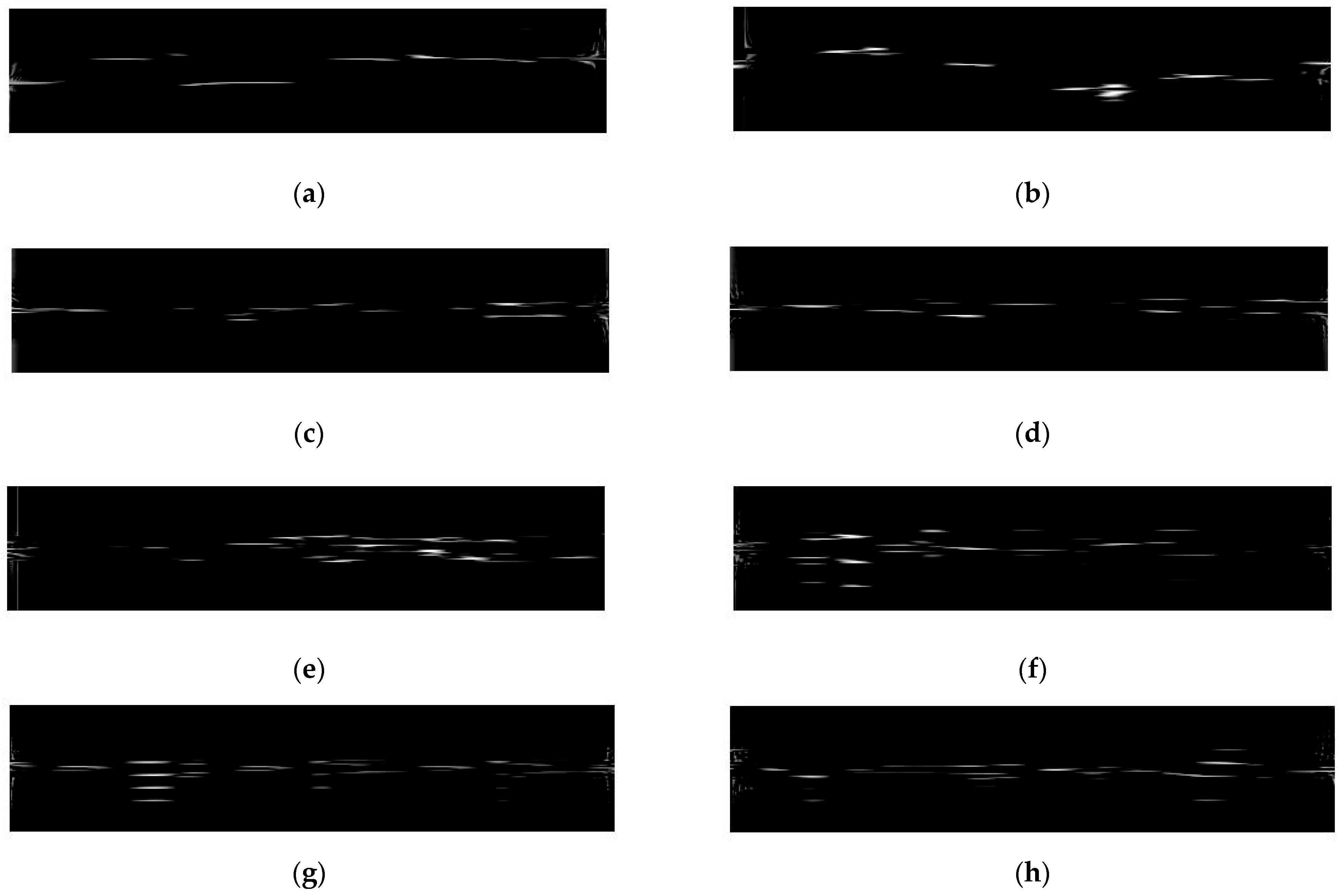
2. UWA Signal Preprocessing
3. Network Model Design
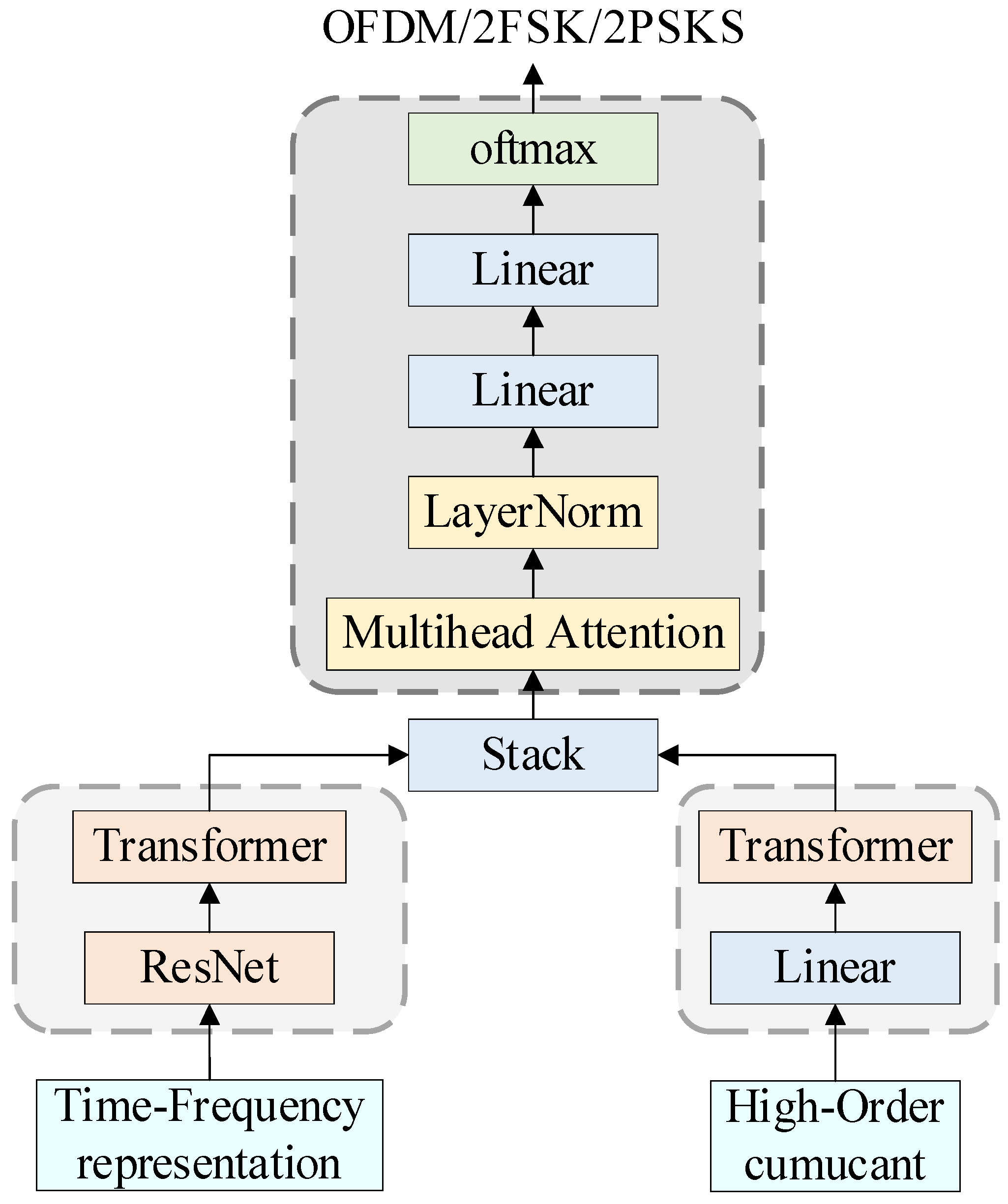
3.1. Methodology
- (1)
- Feature Type Discrepancy: Time–frequency maps are 2D images containing both local structures (e.g., frequency-hopping patterns and energy distributions) and global trends (e.g., periodicity of modulation modes). HOS are low-dimensional vector features derived from signal statistics (e.g., real/imaginary parts of second/fourth-order statistics), reflecting non-Gaussianity and phase information as global statistical properties without local spatial structures.
- (2)
- Network Adaptability: Statistical features, being mathematically transformed statistics without inherent spatial dependencies, are ill-suited for convolutional operations. Thus, ResNet is ineffective for their extraction.
- (3)
- Computational Efficiency: The time–frequency branch employs a dual-network architecture to enhance multi-scale feature extraction, prioritizing expressive power. The statistics branch leverages Transformer’s global modeling capability to efficiently capture statistical correlations, avoiding overfitting from excessive layers.
- (1)
- Effective Feature Fusion:
- (2)
- Nonlinear Expressiveness:
- (3)
- Model Generalization:
3.2. Feature Extraction Layer
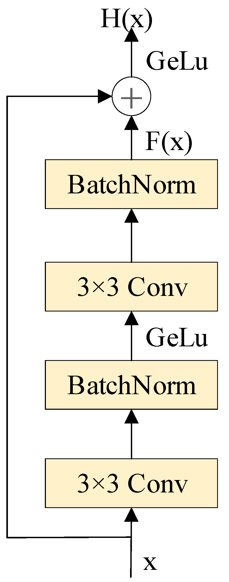
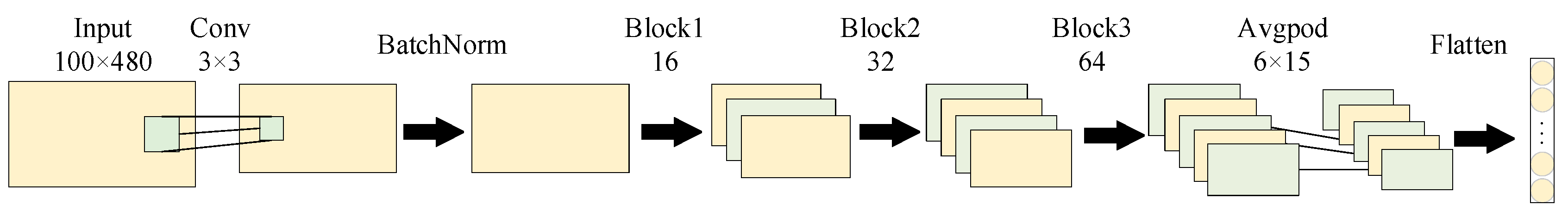
3.2.1. ResNet Model Structure
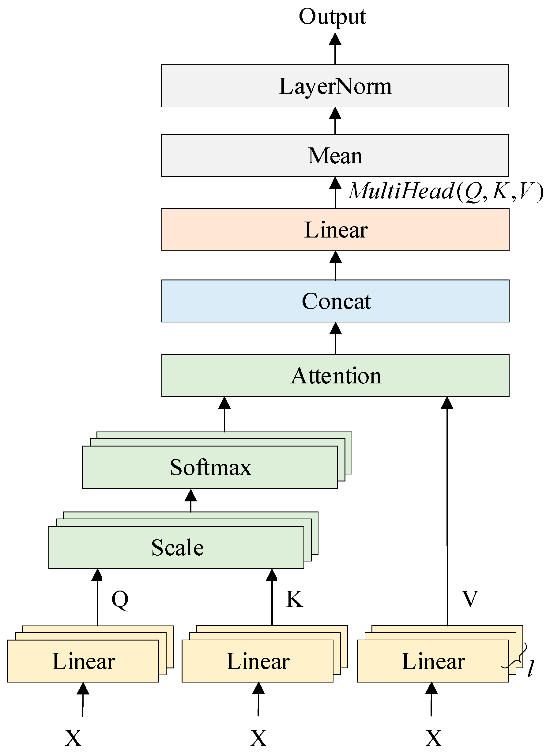
3.2.2. Transformer Model Structure
3.3. Classification Layer
- (1)
- Fusing dual features: Multi-head attention is adopted to fuse time–frequency features and HOS features, resulting in a fused feature dimension of 256.
- (2)
- Linear transformation: Linear transformation is achieved through matrix multiplication and addition operations, mapping the 256-dimensional input features to 128 dimensions.
- (3)
- Nonlinear activation: The GELU activation function is applied to perform the nonlinear transformation on the output of the linear transformation, introducing nonlinearity to enable the model to learn more complex features.
- (4)
- Dropout regularization: During training, a dropout layer is introduced to randomly set a portion of input units to zero, preventing the model from overfitting.
- (5)
- Final classification: Linear transformation is implemented through matrix multiplication and addition operations, mapping the 128-dimensional input features to 8 dimensions to obtain the final classification results.
4. Results
4.1. Datasets
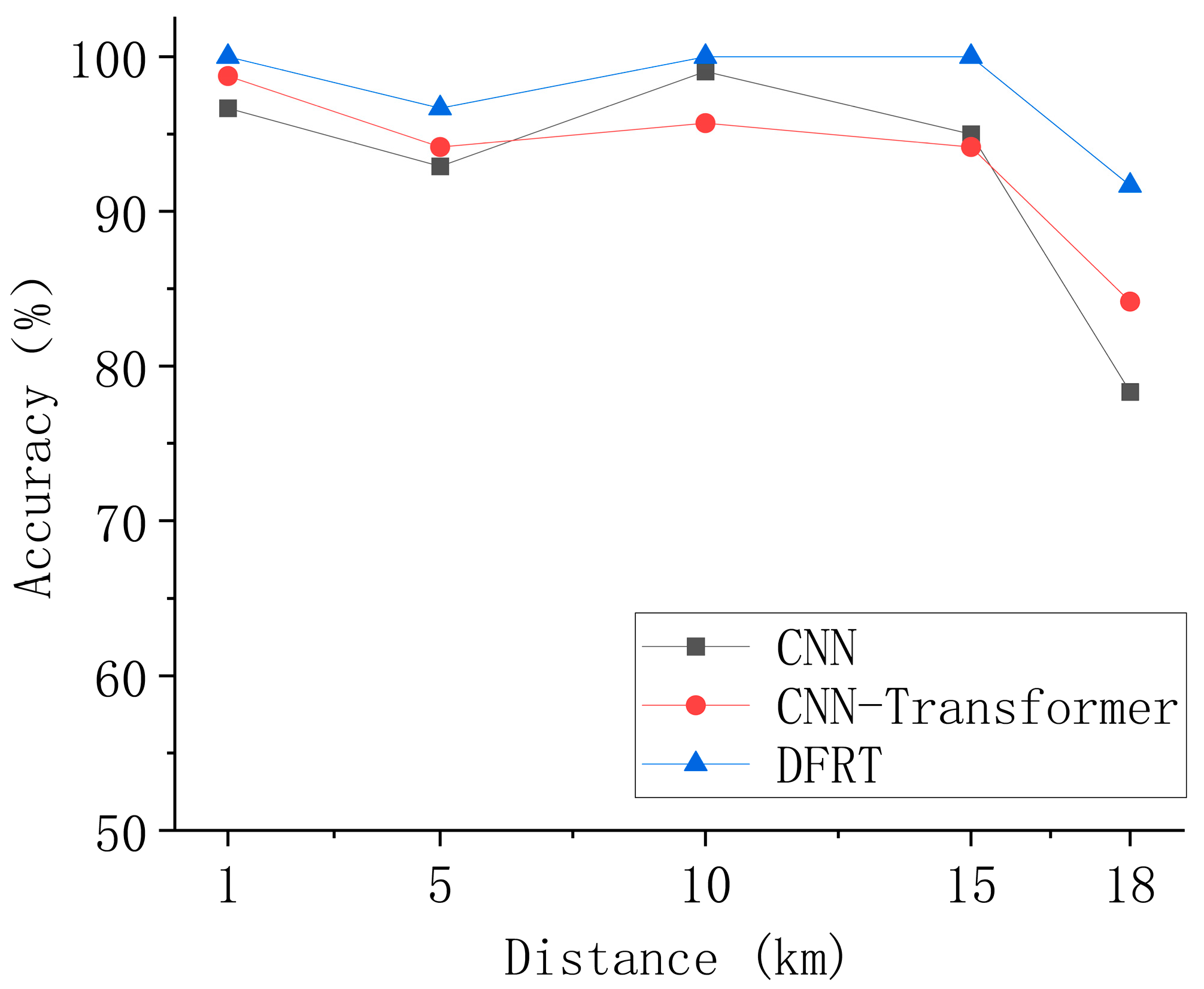
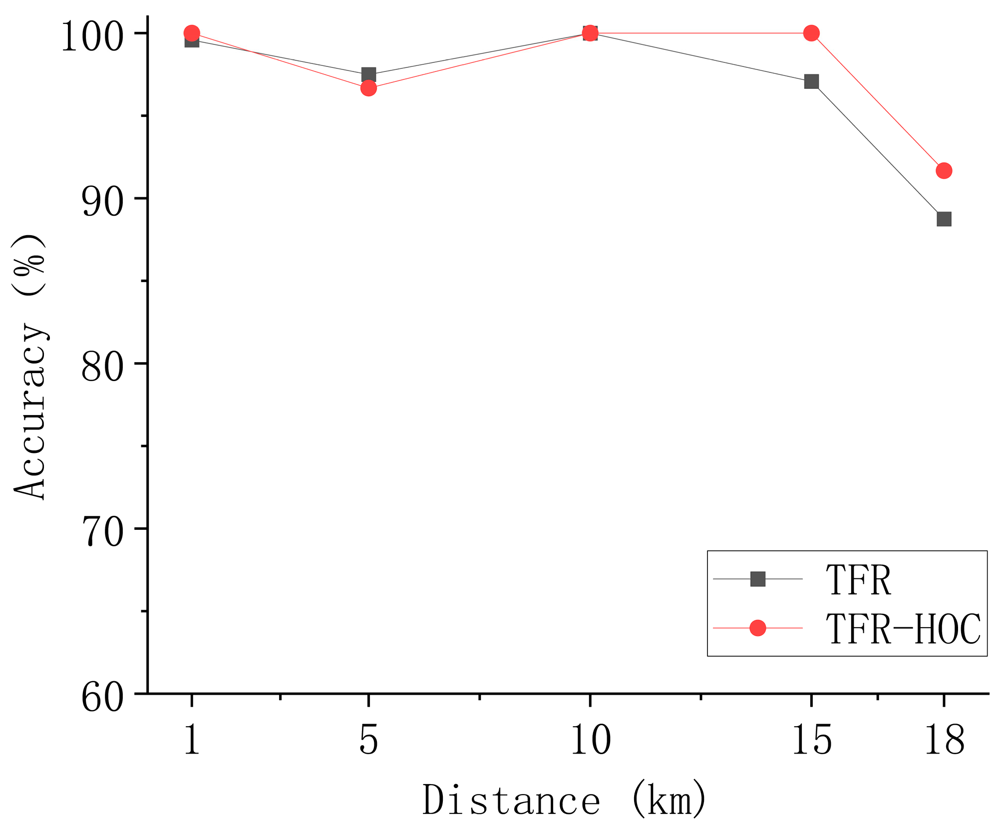
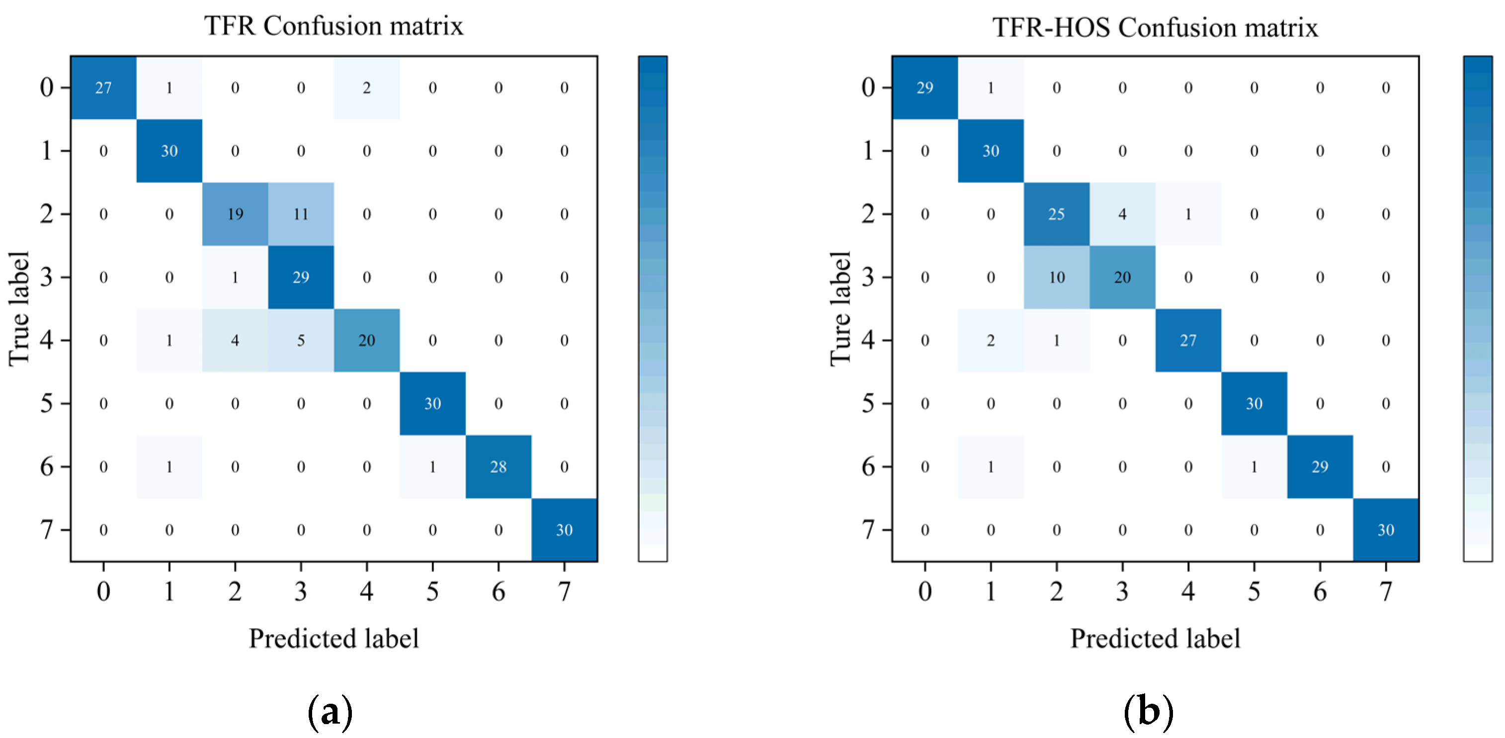
4.2. Analysis
5. Conclusions and Future Work
5.1. Conclusions
5.2. Future Work
- (1)
- Further enhance the model’s robustness in extremely long-distance and dynamic time-varying channels, and improve the extraction of weak phase features by incorporating semi-supervised learning techniques. This will address the challenges of low SNR and phase ambiguity in complex underwater environments.
- (2)
- Expand the coverage of modulation types and develop a multi-task learning framework to achieve joint optimization of modulation recognition and channel estimation. This integrated approach will enhance the model’s versatility across diverse communication protocols.
Author Contributions
Funding
Institutional Review Board Statement
Informed Consent Statement
Data Availability Statement
Conflicts of Interest
Abbreviations
| AMR | Automatic Modulation Recognition |
| CLDNN | Convolutional Long Short-Term Deep Neural Network |
| CNN | Convolutional Neural Network |
| DFRT | Dual Feature ResNet–Transformer |
| DSSS | Direct Sequence Spread Spectrum |
| HOS | Higher-Order Statistics |
| LSTM | Long Short-Term Memory |
| MFSK | Multiple Frequency Shift Keying |
| MPSK | Multiple Phase Shift Keying |
| OFDM | Orthogonal Frequency Division Multiplexing |
| RNN | Recurrent Neural Network |
| SNR | Signal-to-Noise Ratio |
| SPWVD | Smooth Pseudo-Wigner–Ville Distribution |
| STFT | Short-Time Fourier Transform |
| TFR | Time–Frequency Representation |
| TSTR | Two-Stream Transformer |
| UWA | Underwater Acoustic |
| WT | Wavelet Transform |
Notation List
| Mechanism in neural networks that computes a weighted sum of input vectors based on their relevance to a query, enhancing the model’s ability to focus on important features. | |
| Abbreviation for cumulative operations, which compute running totals or products over a sequence. | |
| Mathematical expectation operator, denoting the average value of a random variable over its probability distribution. | |
| Refers to multi-head attention, a technique that splits the input into multiple subspaces and applies parallel attention mechanisms to capture diverse patterns. | |
| Normalization function that converts a vector of raw scores into a probability distribution over multiple class. | |
| Smoothed Pseudo Wigner–Ville Distribution, a time–frequency analysis method that combines the Wigner–Ville distribution with kernel smoothing to reduce cross-terms. | |
| Hyperbolic tangent function, a sigmoidal activation function that maps inputs to the range (−1, 1), often used in recurrent neural networks. | |
| Variance operator, measuring the spread of a random variable’s distribution around its expected value. |
References
- James, P. Acoustic propagation considerations for underwater acoustic communications network development. ACM SIGMOBILE Mob. Comput. Commun. Rev. 2007, 11, 2–10. [Google Scholar]
- Rizwan, K.M.; Das, B.; Pati, B.B. Channel estimation strategies for underwater acoustic (UWA) communication: An overview. J. Frankl. Inst. 2020, 357, 7229–7265. [Google Scholar]
- Nvzhi, T.; Zeng, Q.; Zeng, Q.; Xu, Q. Research on development and application of underwater acoustic communication system. J. Phys. Conf. Ser. 2020, 1617, 012036. [Google Scholar]
- Fang, S. Principles and Techniques of Underwater Acoustic Reconnaissance; Science Press: Beijing, China, 2023; pp. 151–178. [Google Scholar]
- Yao, X.; Yang, H.; Sheng, M. Automatic modulation classification for underwater acoustic communication signals based on deep complex networks. Entropy 2023, 25, 318. [Google Scholar] [CrossRef] [PubMed]
- Ananthram, S.; Sadler, B.M. Hierarchical digital modulation classification using cumulants. IEEE Trans. Commun. 2000, 48, 416–429. [Google Scholar]
- Nadya, H.K.; Mansour, A.; Nordholm, S. Classification of digital modulated signals based on time frequency representation. In Proceedings of the 2010 4th International Conference on Signal Processing and Communication Systems, Gold Coast, QLD, Australia, 13–15 December 2010. [Google Scholar]
- Xu, Z.; Wu, X.; Gao, D.; Su, W. Blind modulation recognition of UWA signals with semi-supervised learning. In Proceedings of the 2022 IEEE International Conference on Signal Processing, Communications and Computing (ICSPCC), Xi’an, China, 25–27 October 2022. [Google Scholar]
- Brahmjit, S.; Jindal, P.; Verma, P.; Sharma, V.; Prakash, C. Automatic Modulation Recognition Using Modified Convolutional Neural Network. In Proceedings of the 2025 3rd International Conference on Device Intelligence, Computing and Communication Technologies (DICCT), Dehradun, India, 21–22 March 2025. [Google Scholar]
- Yogesh, B.; Emilien, D.G.D. A Modified Convolutional Neural Network Model for Automatic Modulation Classification. In Proceedings of the 2025 Emerging Technologies for Intelligent Systems (ETIS), Dehradun, India, 21–22 March 2025. [Google Scholar]
- Ke, Z.; Vikalo, H. Real-time radio technology and modulation classification via an LSTM auto-encoder. IEEE Trans. Wirel. Commun. 2021, 21, 370–382. [Google Scholar] [CrossRef]
- Udaya, D.; Amarasooriya, R.; Samarasinghe, S.M.; Karunasingha, N.A. Combined Classifier-Demodulator Scheme Based on LSTM Architecture. Wirel. Commun. Mob. Comput. 2022, 2022, 5584481. [Google Scholar]
- Zhang, B.; Chen, G.; Jiang, C. Research on modulation recognition method in low SNR based on LSTM. J. Phys. Conf. Ser. 2022, 2189, 012003. [Google Scholar] [CrossRef]
- Zhang, W.; Yang, X.; Leng, C.; Wang, J.; Mao, S. Modulation recognition of underwater acoustic signals using deep hybrid neural networks. IEEE Trans. Wirel. Commun. 2022, 21, 5977–5988. [Google Scholar] [CrossRef]
- West Nathan, E.; O’shea, T. Deep architectures for modulation recognition. In Proceedings of the 2017 IEEE international symposium on dynamic spectrum access networks (DySPAN), Baltimore, MD, USA, 6–9 March 2017. [Google Scholar]
- Cai, J.; Gan, F.; Cao, X.; Liu, W. Signal modulation classification based on the transformer network. IEEE Trans. Cogn. Commun. Netw. 2022, 8, 1348–1357. [Google Scholar] [CrossRef]
- Zhang, W.; Xue, K.; Yao, A.; Sun, Y. CTRNet: An Automatic Modulation Recognition Based on Transformer-CNN Neural Network. Electronics 2024, 13, 3408. [Google Scholar] [CrossRef]
- Li, J.; Jia, Q.; Cui, X.; Gulliver, T.A.; Jiang, B.; Li, S.; Yang, J. Automatic modulation recognition of underwater acoustic signals using a two-stream transformer. IEEE Internet Things J. 2024, 11, 18839–18851. [Google Scholar] [CrossRef]
- Pang, C.; Wang, F.; Chen, M.; Liu, Y.; Dong, Y. Modulation Recognition of Underwater Acoustic Signals Using Dynamic Dilated Convolutional Neural Network and Transformer. In Proceedings of the 2024 IEEE International Conference on Signal, Information and Data Processing (ICSIDP), Zhuhai, China, 22–24 November 2024. [Google Scholar]
- Shin, D.-M.; Park, D.-H.; Kim, H.-N. Deep Learning-Based Modulation Recognition with Multi-Scale Temporal Feature Extraction. In Proceedings of the 2025 International Conference on Information Networking (ICOIN), Chiang Mai, Thailand, 15–17 January 2025. [Google Scholar]
- Dong, Y.; Zhai, R.; Wang, B.; Zhong, Y.; Rong, Z.; Wang, Y. A Novel Distributed Solution for Automatic Modulation Classification Based on Federated Learning and Modified LSTM. IEEE Trans. Veh. Technol. 2025, 1–13. [Google Scholar] [CrossRef]
- Leon, C. Time-Frequency Analysis: Theory and Applications; Pearson College Div: Toronto, ON, Canada, 1995. [Google Scholar]
- Xie, W.; Hu, S.; Yu, C.; Zhu, P.; Peng, X.; Ouyang, J. Deep learning in digital modulation recognition using high order cumulants. IEEE Access 2019, 7, 63760–63766. [Google Scholar] [CrossRef]
- He, K.; Zhang, X. Deep residual learning for image recognition. In Proceedings of the IEEE Conference on Computer Vision and Pattern Recognition, Las Vegas, NV, USA, 27–30 June 2016. [Google Scholar]
- Chen, J.; Zhao, R. Wireless Signal Recognition Based on ResNet-Transformer. In Proceedings of the 2023 11th International Conference on Intelligent Computing and Wireless Optical Communications (ICWOC), Chongqing, China, 16–18 June 2023. [Google Scholar]

| Layer (Type) | Input Shape | Output Shape | Param |
|---|---|---|---|
| Linear | [1, 256] | [1, 128] | 32,896 |
| Gelu | [1, 128] | [1, 128] | 0 |
| Dropout | [1, 128] | [1, 128] | 0 |
| Linear | [1, 128] | [1, 8] | 1032 |
| Modulations | 2FSK, 4FSK, 2PSK, 4PSK, OFDM, DSSS, 4DSSS, 9DSSS |
| Signal format | time domain signal |
| Signal dimension | 1 × 4800 |
| Distance (km) | 1; 5; 10; 15; 18 |
| Total number of samples | 4000 |
| training sets: test sets | 7:3 |
| Advantages | Disadvantages | |
|---|---|---|
| CNN | (1) Simple architecture: Characterized by a small parameter size and high computational efficiency, making it suitable for lightweight scenarios. (2) Local feature sensitivity: Capable of capturing local structures in TFR (e.g., frequency hopping patterns) with reasonable accuracy. | (1) Inadequate long-range dependency modeling: Fails to effectively capture global temporal or frequency domain correlations in signals (e.g., periodicity of modulation patterns). (2) Weak phase information extraction: Results in low classification accuracy for phase-modulated signals (e.g., 2PSK, 4PSK) due to the lack of nonlinear phase feature modeling capability. (3) Gradient degradation issue: Prone to gradient vanishing in deep networks, limiting the ability to learn complex features. |
| CNN–Transformer | (1) Enhanced global feature capture capability: Compared to single CNN, it can extract long-range dependencies through Transformer’s self-attention mechanism. (2) Attempt at multi-modal feature fusion: Integrates TFR with shallow statistical features to improve recognition accuracy for complex modulations. | (1) High design complexity: The hybrid architecture requires coordinating parameters between convolutional and Transformer modules, increasing training complexity and potentially necessitating larger datasets or more sophisticated parameter tuning strategies. (2) Unresolved gradient degradation: Training difficulties persist in deep networks due to the absence of residual connections. |
| DFTR | (1) Effective gradient degradation mitigation: The ResNet residual connections ensure training stability in deep networks. (2) Enhanced phase feature extraction: HOS directly captures signal non-Gaussianity and phase information, compensating for the insensitivity of TFR to phase. (3) Global–local feature collaboration: Transformer models long-range dependencies, while ResNet extracts local details, jointly enhancing robustness in complex scenarios. (4) Dynamic feature fusion: The multi-head attention mechanism automatically adjusts feature weights according to task requirements, avoiding the limitations of fixed fusion. | (1) Higher computational complexity: The dual-branch structure and multi-head attention mechanism result in a larger parameter size compared to single CNN or Transformer models. (2) Strong data dependency: HOS extraction is dependent on high-quality signal preprocessing, requiring more complex denoising processing under low-SNR conditions. |
Disclaimer/Publisher’s Note: The statements, opinions and data contained in all publications are solely those of the individual author(s) and contributor(s) and not of MDPI and/or the editor(s). MDPI and/or the editor(s) disclaim responsibility for any injury to people or property resulting from any ideas, methods, instructions or products referred to in the content. |
© 2025 by the authors. Licensee MDPI, Basel, Switzerland. This article is an open access article distributed under the terms and conditions of the Creative Commons Attribution (CC BY) license (https://creativecommons.org/licenses/by/4.0/).
Share and Cite
Zhou, F.; Wu, H.; Yue, Z.; Li, H. An Underwater Acoustic Communication Signal Modulation-Style Recognition Algorithm Based on Dual-Feature Fusion and ResNet–Transformer Dual-Model Fusion. Appl. Sci. 2025, 15, 6234. https://doi.org/10.3390/app15116234
Zhou F, Wu H, Yue Z, Li H. An Underwater Acoustic Communication Signal Modulation-Style Recognition Algorithm Based on Dual-Feature Fusion and ResNet–Transformer Dual-Model Fusion. Applied Sciences. 2025; 15(11):6234. https://doi.org/10.3390/app15116234
Chicago/Turabian StyleZhou, Fanyu, Haoran Wu, Zhibin Yue, and Han Li. 2025. "An Underwater Acoustic Communication Signal Modulation-Style Recognition Algorithm Based on Dual-Feature Fusion and ResNet–Transformer Dual-Model Fusion" Applied Sciences 15, no. 11: 6234. https://doi.org/10.3390/app15116234
APA StyleZhou, F., Wu, H., Yue, Z., & Li, H. (2025). An Underwater Acoustic Communication Signal Modulation-Style Recognition Algorithm Based on Dual-Feature Fusion and ResNet–Transformer Dual-Model Fusion. Applied Sciences, 15(11), 6234. https://doi.org/10.3390/app15116234