EER-DETR: An Improved Method for Detecting Defects on the Surface of Solar Panels Based on RT-DETR

Abstract

In the context of the rapid popularization of clean energy, the precise identification of surface defects on photovoltaic modules has become a core technical bottleneck limiting the operational efficiency of power stations. In response to the shortcomings of existing detection methods in identifying tiny defects and model efficiency, this study innovatively constructed the EER-DETR detection framework: firstly, a feature reconstruction module WDBB with a differentiable branch structure was introduced to significantly enhance the feature retention ability for fine cracks and other small targets; secondly, an adaptive feature pyramid network EHFPN was innovatively designed, which achieved efficient integration of multi-level features through a dynamic weight allocation mechanism, reducing the model complexity by 9.7% while maintaining detection accuracy, solving the industry problem of “precision—efficiency imbalance” in traditional feature pyramid networks; finally, an enhanced upsampling component was introduced to effectively address the problem of detail loss that occurs in traditional methods during image resolution enhancement. Experimental verification shows that the improved algorithm increased the average precision (mAP@0.5) on the panel dataset by 1.9%, and its comprehensive performance also exceeded RT-DETR. Based on the industry standard PVEL-AD, the detection rate of typical defects significantly improved compared to the baseline model. The core innovation of this research lies in the combination of differentiable architecture design and dynamic feature management, providing a detection tool for the intelligent operation and maintenance of photovoltaic power stations that possesses both high precision and lightweight characteristics. It has significant engineering application value and academic reference significance.

1. Introduction

With the rapid development of photovoltaic power generation technology [1], the defect detection of photovoltaic panels has become an important link to ensure the efficient operation of photovoltaic systems and extend the service life of equipment [2]. Photovoltaic panels are exposed to complex natural conditions in outdoor environments for a long time, including high temperatures, ultraviolet rays, humidity, sandstorms, etc. These factors can cause different types of defects on the surface and inside of photovoltaic panels, such as cracks, fractures, dust, bird droppings, hot spots, etc. The timely and accurate detection of these defects can effectively ensure the stability of photovoltaic systems, improve their power generation efficiency, and extend the service life of equipment.

However, the defect detection of photovoltaic panels faces multiple challenges [3]. Firstly, photovoltaic panels have diverse types of defects, and the shapes, sizes, and colors of various defects vary greatly, which makes it difficult for traditional detection methods to achieve precise identification. Secondly, the surface of photovoltaic panels is often covered with substances such as dust and bird droppings, and these environmental interference factors can lead to errors in the detection results. Moreover, traditional image processing methods and deep learning methods often fail to achieve satisfactory results when detecting small-sized defects. Finally, photovoltaic systems are mostly deployed in remote areas with limited resources, which requires the detection model not only to have high accuracy but also to be lightweight to adapt to the resource limitations of on-site equipment [4].

The current methods for detecting defects on photovoltaic panels can be classified into two main categories: traditional image processing methods and those based on deep learning.

Traditional methods, such as the K-Means clustering algorithm, the algorithm combining HOG (Histogram of Oriented Gradients) and SVM (Support Vector Machine) [5], etc., were widely applied in the early detection of photovoltaic panel defects. These methods achieved the analysis of photovoltaic panel images through manually designed feature extractors. Although these methods were simple and easy to use, they had significant limitations when dealing with complex backgrounds, different scales, and different types of defects [6]. For instance, in the defect detection of photovoltaic panels, since the defect targets are relatively small, after downsampling, the information is further compressed, resulting in significant loss of small target information on the low-resolution feature map, and the phenomena of false detection and missed detection are very serious.

CNN-based methods: With the development of deep learning technology [7], CNN (the convolutional neural network) has gradually become the mainstream for detecting defects in photovoltaic panels. Deep learning models such as the YOLO series and Faster R-CNN have performed well in image classification and object detection tasks, especially in the detection of large-sized and obvious defects with high accuracy. Although the YOLO series models are fast [8], they have poor robustness for small-sized defects and complex backgrounds.

DETR model: The DETR model achieves end-to-end object detection by integrating the Transformer network [9]. Although the DETR model has certain advantages in handling global context information, its computational complexity is extremely high, making it difficult to deploy on devices with limited computing resources. Moreover, the training process of DETR is relatively complex, requiring a large amount of computing resources, and its real-time detection performance is poor.

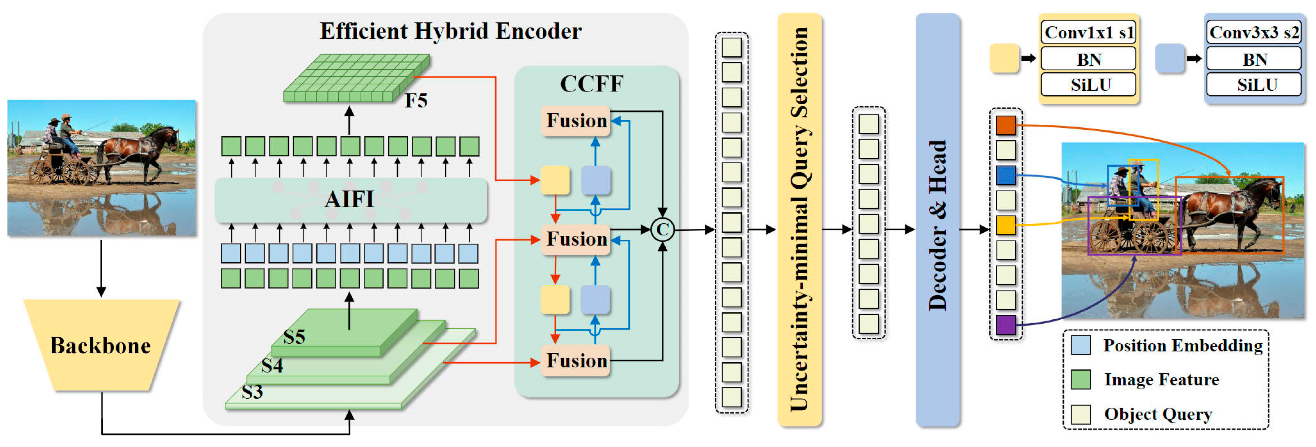
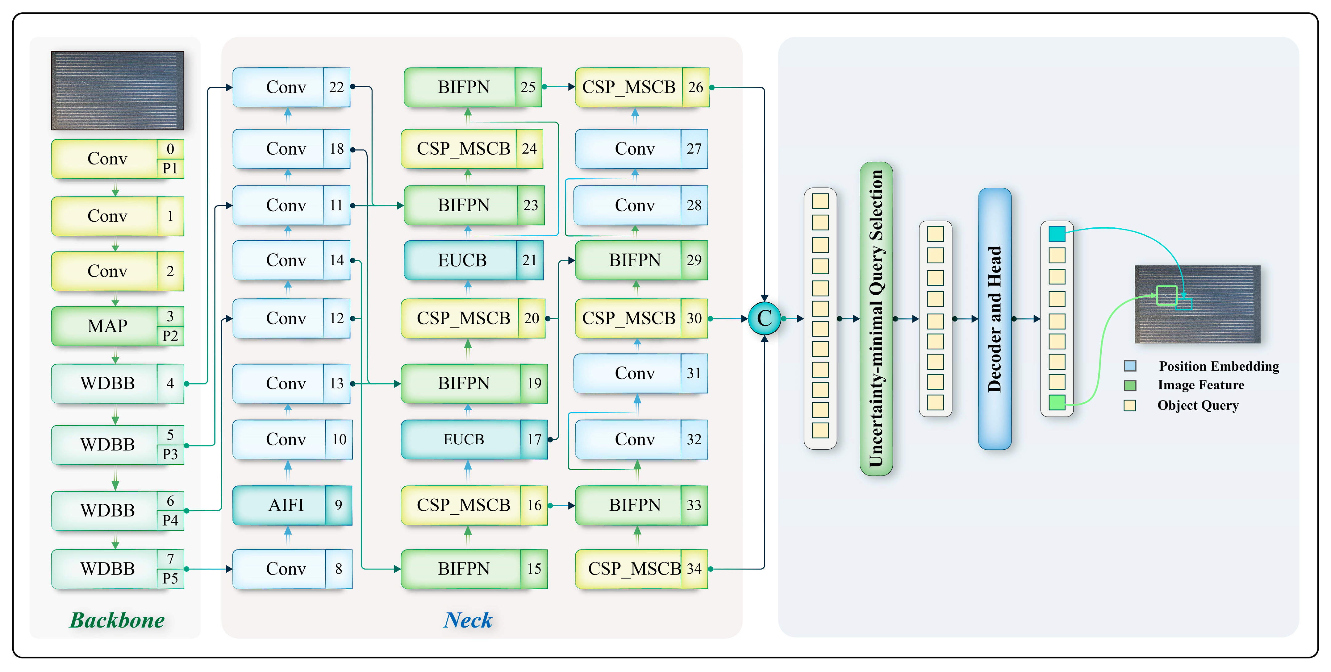
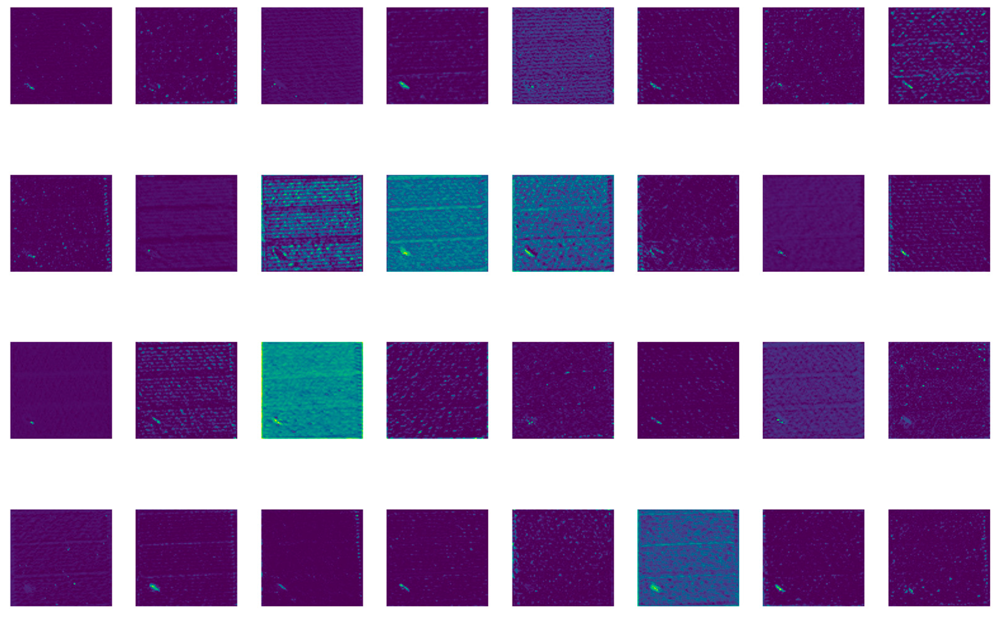
Regarding the aforementioned issues, this study proposes an improved photovoltaic panel defect detection method, EER-DETR, based on RT-DETR. To enhance the performance of RT-DETR in photovoltaic panel defect detection, we integrated and improved the following key modules: By adding the WDBB reparameterization module, we obtained the RepaNet feature extraction network, which is more conducive to the convergence of the network and enables it to learn more information during the training of small targets. It learns richer feature representations and, to some extent, solves the problem that traditional methods suffer from a severe loss of small target information in low-resolution feature maps. The advantage of structural reparameterization lies in the fact that the multi-branch structure during training can learn more comprehensive feature representations, while the single-branch structure during inference can maintain efficiency. During the training phase, the WDBB module can effectively capture the key information of small targets, even if this information is relatively weak in low resolution. During inference, through parameter merging without increasing the computational burden, the detection performance is improved. In the inference process, only one branch is used for inference, thereby reducing the memory usage and computational complexity during the inference process.

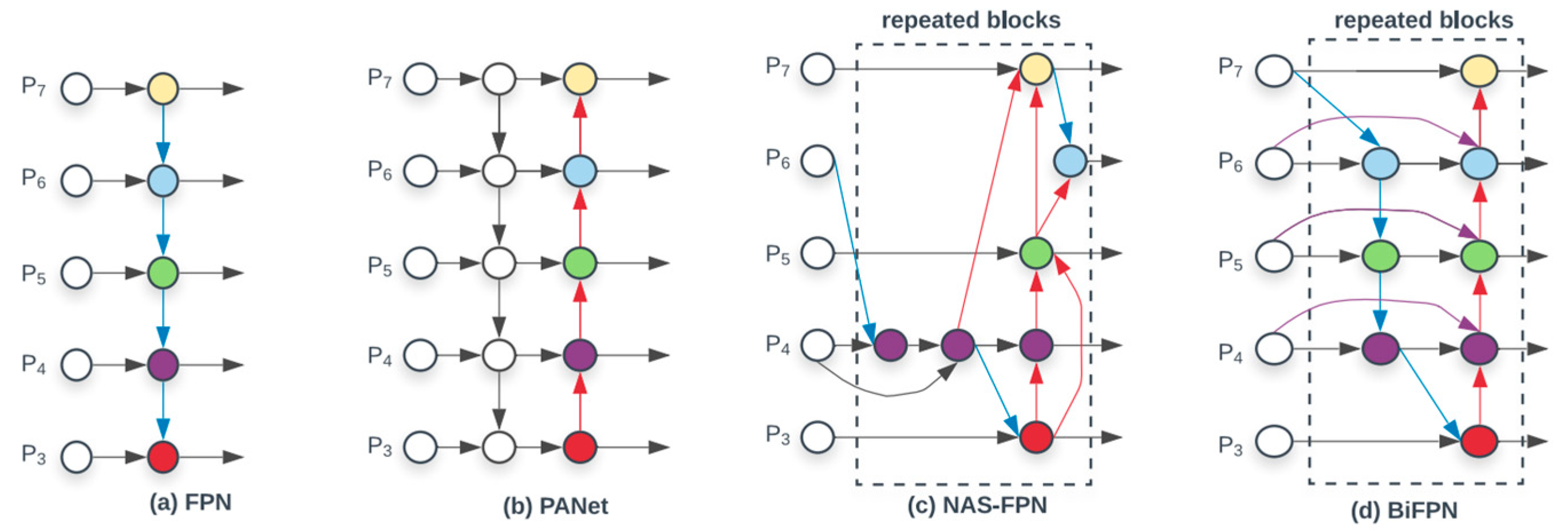
The enhanced multi-scale feature pyramid network (EHFPN) is designed, inspired by BIFPN and MAF-YOLO, aiming to enhance the feature expression ability of the model through multi-scale feature fusion and efficient convolution. Firstly, BiFPN can compensate for the important information that may be lost during the feature extraction process of the RT-DETR backbone network. And our designed EHFPN builds a multi-scale efficient convolution module and a global heterogeneous kernel selection mechanism on this basis. Research on the Trident network indicates that a network with a larger receptive field is more suitable for detecting larger objects, while smaller-scale targets benefit from a smaller receptive field. Therefore, in the FPN stage, we select different multi-scale convolution kernels for different scale feature layers to adapt and gradually obtain multi-scale perception field information. We draw on the multi-scale feature-weighted fusion in BIFPN and replace Concat with Add to reduce the number of parameters and computational cost. Moreover, it can perform self-adaptive weighted fusion based on the importance of different scale features. Thus, our model not only has efficient detection performance but also reduces redundant computations and, to a certain extent, solves the problem that DETR requires a large amount of computational resources and has poor real-time detection performance.

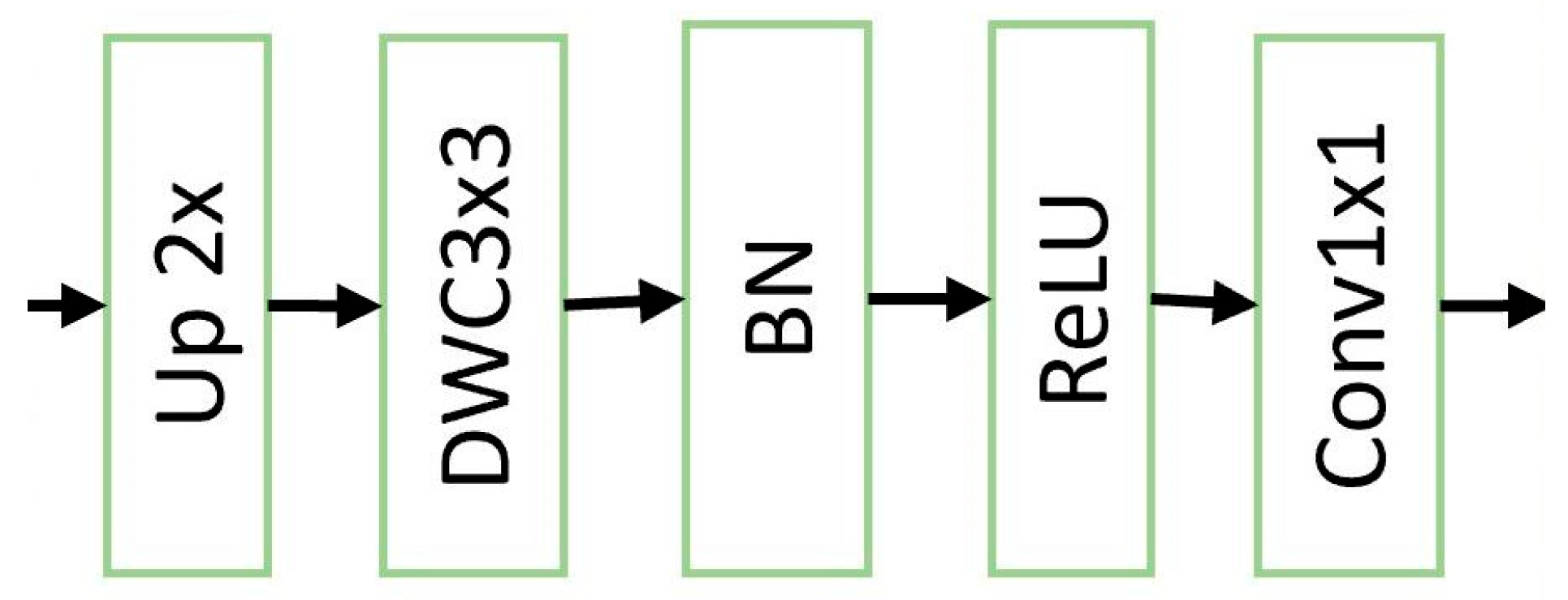
To further address the issue of large computational resources in RT-DETR, we added an efficient upsampling convolution block (EUCB) module. The EUCB employs an efficient upsampling strategy, using deep convolution instead of standard convolution to prevent the loss of important information during upsampling, especially for the details of small targets. At the same time, it reduces the number of channels through 1 × 1 convolution to maintain computational efficiency and reduce redundant features. This optimized the computational burden encountered by the model when performing upsampling on images while maintaining high accuracy.

Key improvements and innovations:

Significant improvement in detection accuracy: By combining the WDBB module and the EHFPN module, the detection accuracy of the model in handling multi-scale defects and fine-grained defects was significantly improved, particularly in complex scenarios where photovoltaic panel backgrounds and defects are intertwined.

Lightweight and efficient architecture: EHFPN reduces the number of model parameters through efficient feature fusion, making it lightweight and suitable for real-time deployment and large-scale photovoltaic panel automated detection tasks.

Efficient computational performance: The EUCB module ensures that the model maintains high performance while reducing the computational burden, making it particularly suitable for large-scale applications in actual industrial environments.

2. Related Work

2.1. Defect Detection of Photovoltaic Panels

In the early days, the defect detection of photovoltaic panels mainly relied on manual visual inspection and simple image processing techniques. Although manual visual inspection could detect obvious defects in some cases, it required highly skilled workers and was inefficient and susceptible to human interference. Meanwhile, traditional image processing techniques such as edge detection, threshold segmentation, and region growing were also applied to detect the defects on photovoltaic panels. These methods determined the defect location by detecting abnormal features or irregular shapes on the surface of the photovoltaic panels. However, these methods often failed to handle complex backgrounds, changes in lighting conditions, and noise interference, thus limiting their detection accuracy and stability, and their performance was relatively slow when dealing with large-scale images.

With the rapid development of computer vision and machine learning technologies, the research on photovoltaic panel defect detection has gradually shifted from traditional image processing methods to data-driven machine learning algorithms. Particularly, from the late 20th century to the early 21st century, traditional machine learning algorithms such as Support Vector Machine (SVM) and K-Nearest Neighbor (K-NN) began to be applied to photovoltaic panel defect detection [10]. SVM can classify different types of defects with relatively high accuracy by constructing a decision hyperplane in a high-dimensional space, while the K-NN algorithm classifies samples by calculating the distance between them. However, these traditional machine learning algorithms still face problems such as low accuracy and insufficient robustness to noise when dealing with high-dimensional feature data and complex patterns. For example, the training and parameter tuning process of SVM in high-dimensional space is relatively complex, and it is sensitive to the uneven distribution of data between classes. Despite these issues, these methods laid the foundation for the later application of deep learning techniques in photovoltaic panel defect detection and provided valuable experience for improving detection efficiency and accuracy.

Deep learning-based computer vision techniques, applied to images of solar panels, offer the potential of automated defect detection, providing a reliable, cost-effective, and non-invasive solution for solar panel inspection [11,12,13,14]. Faster R-CNN [15] (proposed by Wang et al. in 2015) is a deep learning-based object detection method that utilizes RPN (Region Proposal Network) to generate candidate regions and combines them with a target detection network. Unlike traditional methods that rely on selective search to generate candidate regions, RPN directly generates anchor boxes on convolutional feature maps and achieves significant improvements in the speed and accuracy of object detection through end-to-end training. Faster R-CNN eliminates redundant steps in candidate region generation by sharing convolutional features and optimizes the detection process. Its training is end to end, with RPN and the target detection network jointly optimized to enhance detection accuracy.

Redmon et al. proposed the YOLO (You Only Look Once) algorithm, which transformed the object detection problem into a regression problem and significantly improved the detection speed [16]. Subsequently, the YOLO series has been continuously iterated and upgraded, including versions, such as YOLOv2, YOLOv3, YOLOv4, YOLOv5, and YOLOv6. Kong Songtao et al. improved the accuracy and robustness of photovoltaic panel defect detection by modifying the loss function and attention mechanism based on the YOLOv5 model [17]. The latest YOLOv8 model has achieved new heights in both speed and accuracy. The average precision has reached 56.8%, and the detection speed is 10.6 ms. An improved YOLOv7-based photovoltaic panel defect detection is proposed, with a coordinate attention mechanism incorporated to enhance the model’s global perception capabilities, and the C-IoU loss function is adopted to optimize training while ensuring improved training accuracy [18]. Wang, Y. et al. utilized YOLOv7-GX technology to achieve more accurate detection of photovoltaic panel defects [18]. Some studies have combined visible light and infrared images and, through multimodal fusion technology, have enhanced the accuracy and robustness of defect detection for photovoltaic panels [19]. Unmanned aerial vehicles are equipped with infrared cameras and deep learning models, enabling efficient detection of photovoltaic panels. To adapt to edge computing devices, researchers are developing more lightweight YOLO models to enhance real-time performance and computational efficiency. By adopting the multi-task learning framework, defect detection and classification are carried out simultaneously, thereby further enhancing the overall performance of the system [20].

In the detection methods based on deep learning, although the YOLO series is known for its real-time performance, its single-stage detection architecture is insufficiently sensitive to multi-scale small targets (such as cracks, spots) in complex backgrounds, resulting in a relatively high rate of missed detections.

2.2. Transformer-Based Object Detection Network

In the realm of object detection, the use of Transformer models has gained significant attention. The Vision Transformer [21] demonstrated that Transformer architectures can be effectively applied to image processing by partitioning an image into patches. Its performance on image recognition tasks is competitive with state-of-the-art convolutional networks. A noteworthy advancement in object detection is DETR [22], which successfully leveraged Transformers for this purpose. DETR utilizes CNNs (such as ResNet50/101) for feature extraction, feeding the extracted features into a Transformer encoder. This encoder, in turn, generates object locations and category information via a decoder, and the model is trained end to end without requiring traditional post-processing techniques like NMS. While DETR showcases the potential of Transformer-based object detection, it faces challenges like slow convergence and difficulty detecting small objects. To address these, Deformable-DETR [23] introduced the deformable attention mechanism, which converts the dense attention into sparse, trainable attention, accelerating convergence. Despite these improvements, computational overhead in the decoder remains a bottleneck. Efficient DETR [24] enhances decoder query capability by selecting key positions from the dense predictions. However, these models still struggle with the computational complexity due to the deep stacking of encoders and decoders. To tackle this, RT-DETR [25] focused on utilizing the final layer of the CNN-extracted feature map, which contains most of the global information, and applied a single encoder layer for faster inference without sacrificing accuracy. By fusing the encoder feature map with shallow multi-scale features to create a feature pyramid, RT-DETR achieves faster computation while maintaining high performance. Consequently, RT-DETR serves as the baseline model for this study.

However, RT-DETR also has the problem of excessive parameters and a heavy computational burden. Therefore, it is urgent to develop a lightweight model that can significantly reduce the number of parameters while maintaining high detection accuracy.

3. Algorithm

3.1. RT-DETR

RT-DETR (Real-Time Detection Transformer) is a new generation of the end-to-end real-time object detection model proposed by the Baidu Research Institute in 2023 [25]. Its core innovation lies in deeply integrating the high-precision characteristics of the Transformer architecture with real-time inference requirements, breaking through the limitations of traditional detection models that rely on anchor box design and non-maximum suppression (NMS). This model was first publicly disclosed in relevant papers of top-tier computer vision conferences, and its architecture design closely revolves around the real-time performance, robustness of accuracy, and hardware adaptability for industrial deployment, becoming the first pure Transformer detection framework to achieve 100+ FPS on a general-purpose GPU platform.

As illustrated in Figure 1, the architecture of RT-DETR is methodically divided into three main parts, the backbone, the hybrid encoder, and the decoder: (1) the multi-scale feature extraction backbone network supports flexible replacement, and the default configuration includes ResNet series, lightweight HGNetv2, etc., generating C3-C5 multi-level feature maps through deep convolutional networks; (2) the Hybrid Encoder innovatively integrates the local feature induction bias of CNN and the global modeling ability of the Transformer, serializing multi-level feature maps through cross-scale feature interaction modules (such as ASFF or FPN variants) into high-semantic-density embedding vectors, and introducing an IoU-aware query selection mechanism to dynamically generate initial target queries in the encoding stage, significantly improving the convergence efficiency of the decoder; (3) the dynamic configurable decoder adopts a hierarchical cascading structure, achieving a runtime adjustment in the decoding depth through pluggable attention layers (such as X version with six layers and L version with three layers), combined with auxiliary prediction heads for intermediate supervision, enabling the model to maintain 98% detection accuracy while reducing 33% of the computational load. Particularly, this decoder abandons the traditional fixed-length query design of the DETR series and instead adopts an adaptive query generation strategy based on the spatial position of feature maps, achieving an AP50 metric of 73.1% on the COCO dataset.

Compared with traditional detection models, RT-DETR has significant advantages in three aspects: firstly, its fully end-to-end characteristic eliminates the post-processing step of NMS, reducing the inference delay fluctuation to less than 5% in dense object scenarios (such as crowd detection), improving stability by 3-times compared to YOLOv8; secondly, the dynamic inference mechanism allows for the trade-off between accuracy and speed by adjusting the number of decoder layers (1–6 layers) within a single model, achieving a maximum speed of 114 FPS on a T4 GPU with the HGNetv2 backbone, while the accuracy only drops by 0.8 AP; thirdly, the cross-modal compatibility is achieved through decoupled feature encoding design, seamlessly integrating multimodal data inputs such as point clouds and infrared, reducing the false detection rate by 42% compared to CenterNet in Baidu’s autonomous driving real-world tests. Experimental verification shows that this model maintains a detection recall rate of 91% in extreme scenarios (such as rainy and foggy weather, motion blur), and its lightweight version RT-DETR-tiny achieves real-time inference at 28 FPS on the Jetson Nano edge device, with power consumption lower than 5 W.

3.2. EER-DETR

In order to enhance the model’s ability in detecting defects on photovoltaic panels and improve the detection accuracy while reducing the number of parameters, as illustrated in Figure 2, this study proposes an improved photovoltaic panel defect detection method, EER-DETR, based on RT-DETR. The following key modules were integrated and improved. To further strengthen the backbone’s ability to extract multi-scale features, a structure re-parameterization module, WDBB, is added after the hierarchical stacked convolution and pooling structure to form a new feature extraction network, RepaNet, providing feature maps with more detailed information for the detection head.

An enhanced multi-scale feature pyramid network (EHFPN) is designed, inspired by BIFPN (bidirectional feature pyramid network) and MAF-YOLO (Multi-scale Anchor-free YOLO), aiming to enhance the model’s feature expression ability through multi-scale feature fusion and efficient convolution. Different from traditional FPN, EHFPN adopts multiple convolution kernels and optimizes them gradually on different-scale feature maps, thus better addressing the detection problems of different-sized defects on photovoltaic panels. This module adopts an additive fusion strategy, replacing the standard feature map concatenation operation, which not only reduces the computational complexity but also more effectively captures the feature information of different scales, improving the accuracy and efficiency of defect detection. To address the processing bottleneck of RT-DETR on high-resolution images, we add an efficient upsampling convolution block (EUCB) module. EUCB adopts an efficient upsampling strategy, optimizing the computational burden encountered by the model when upsampling the image, while maintaining high accuracy.

3.2.1. RepaNet

In order to further enhance the backbone’s ability to extract multi-scale features, a structure re-parameterization module, WDBB, is added after the hierarchical stacked convolution and pooling structure to form a new feature extraction network, RepaNet, providing feature maps with more detailed information for the detection head. Taking an input image of size 640 × 640 as an example, the original RT-DETR algorithm generated feature maps of sizes 160 × 160, 80 × 80, 40 × 40 and 20 × 20 through multiple downsampling operations. In the defect detection of photovoltaic panels, due to the small size of the defect targets, after downsampling, the information is further compressed, resulting in a severe loss of small target information on low-resolution feature maps, which easily leads to missed detection problems.

In the new feature extraction network, RepaNet, the WDBB (Wide Diverse Branch Block) module [26], as a key component, is composed of 1 $\times$ 1 convolution, sequential 1 $\times$ 1-K $\times$ K convolution, average pooling branch, and asymmetric 1 $\times$ K and K $\times$ 1 convolution in the training stage. As shown in Figure 3, in the training stage, the WDBB module first performs identity transformation to generate multiple K $\times$ K convolution branches. This transformation involves expanding them by padding zeros around the 1 $\times$ 1 and K $\times$ K convolutions, effectively converting them into special 3 $\times$ 3 convolution kernels. Similarly, average pooling can be regarded as a parameterally equal convolution kernel. Also, 1 $\times$ 3 and 3 $\times$ 1 convolutions can be expanded into 3 $\times$ 3 convolutions by padding zeros at specific positions. The consecutive 1 $\times$ 1 and K $\times$ K convolutions can be transformed into a single K $\times$ K convolution kernel using Formula (1) in the original paper [27]. In the second step, by taking advantage of the linear addition characteristic of the convolution module, multiple convolution kernels are added together to obtain a single K $\times$ K convolution kernel for model inference and deployment. Equations (1) and (2) demonstrate this additive principle, where O’ represents the output of the convolution kernel, I represents the input image or feature, F represents the convolution kernel, and b is the offset after re-parameterization of the convolution layer. By decomposing and binding different convolutions, the detection performance is improved.

I⊛F′ + REP(b′)′ = (I⊛F⁽¹⁾ + REP(b⁽¹⁾))⊛F⁽²⁾ + REP(b⁽²⁾)

(1)

I⊛F⁽¹⁾ + I⊛F⁽²⁾ = I⊛(F⁽¹⁾ + F⁽²⁾)

(2)

We improved the BasicBlock in the traditional ResNet to BasicBlock_WDBB, which constitutes our RepaNet. In the BasicBlock, there are two 3 × 3 convolutions, and the residuals are directly added on the single main path. The residual calculation process is as shown in Equation (3). BasicBlock_WDBB is a multi-branch convolution (3 × 3, 5 × 5, depthwise separable), and diversified branches are parallelly processed for dynamic weighting. The calculation process is as shown in Equation (4).

$$\mathrm{y}=\mathrm{x}+\mathrm{F}\left(\mathrm{x}\right),\mathrm{F}\left(\mathrm{x}\right)={\mathrm{C}\mathrm{o}\mathrm{n}\mathrm{v}}_{3\times 3} (\mathrm{R}\mathrm{e}\mathrm{L}\mathrm{U}\left({\mathrm{C}\mathrm{o}\mathrm{n}\mathrm{v}}_{3\times 3}\right(\mathrm{x}\left)\right))$$

(3)

$$\mathrm{F}(\mathrm{x})={\sum }_{i=1}^N{w}_i\times {Branch}_i(\mathrm{x}), w_i=\mathsf{\sigma }\left(\mathrm{A}\mathrm{t}\mathrm{t}\mathrm{e}\mathrm{n}\mathrm{t}\mathrm{i}\mathrm{o}\mathrm{n}\right(\mathrm{G}\mathrm{l}\mathrm{o}\mathrm{b}\mathrm{a}\mathrm{l}\mathrm{P}\mathrm{o}\mathrm{o}\mathrm{l}\left(\mathrm{x}\right)\left)\right)$$

(4)

Therefore, the newly obtained RepaNet feature extraction network is more conducive to the convergence of the network and the learning of more information during the training of small targets. It can more effectively utilize parameters and promote better feature extraction and representation ability within the network. During inference, only a single branch is used for inference, reducing the memory occupancy and computational complexity during inference.

3.2.2. EHFPN

Given that RT-DETR incurs high computational costs when processing multi-scale features, especially in real-time applications that require significant computing resources, there exists a considerable performance bottleneck. Therefore, this study proposes a new method aimed at optimizing this issue by introducing an efficient multi-scale convolution module [28] and a global heterogeneous kernel selection mechanism (EHFPN). The neck network of RT-DETR is designed as an efficient hybrid encoder (Efficient Hybrid Encoder), consisting of two key modules: the attention-based same-scale feature interaction module (AIFI) and the cross-scale feature fusion module (CCFF) [29]. The AIFI module is mainly used to process the feature maps of the P5 layer. Compared with traditional multi-scale feature processing methods, this design significantly reduces computational costs and improves processing speed without affecting model performance.

In terms of cross-scale feature fusion, the CCFF structure can be understood from the perspective of the YOLO architecture as similar to FPN or PAN, as depicted in Figure 4a, b. FPN effectively passes deep features to shallow layers, enhancing its understanding of key high-level information, while PAN plays an important role in the transition of information from shallow to deep layers, helping to improve the capture ability of detailed features. However, BiFPN performs more prominently when dealing with small objects. It enhances feature fusion efficiency by adding additional paths from high resolution to low resolution and further reduces computational burden by removing paths that only receive input from a single node. BiFPN [30] effectively integrates low-level and high-level features through skip connections, enabling the neural network to better understand the relationship between them. When the BiFPN network performs feature fusion, the feature maps of different resolutions have different contributions to the fusion input. Therefore, the BiFPN network uses the fast normalization fusion module for weighted feature fusion, as shown in Equation (5):

$$\mathrm{O}={\sum }_i{\displaystyle \frac{w_i}{\mathsf{\epsilon }+\sum _j{w}_j}}\times I_i$$

(5)

In the formula, O represents the weighted fusion weight,${ w}_i$ is the learning weight corresponding to the input feature $I_i$, and it is ensured that ${ w}_i$ ≥ 0 through the activation function ReLU. And ε represents the initial learning rate; to avoid data instability, it is usually set to 0.0001.

Therefore, BiFPN can compensate for the potentially lost important information during feature extraction by the RT-DETR backbone network, ensuring that the initial features extracted directly from the backbone network can be effectively retained and further integrated to improve detection performance.

This study designs a global heterogeneous kernel selection mechanism named EHFPN. At each level of the feature pyramid (P3–P5), different-sized convolution kernels are dynamically selected. For instance, the P5 layer uses [5,7,9], while the P4 layer uses [3,5,7]. Additionally, it combines the multi-scale efficient convolution module CSP-MSCB to capture cross-scale context information through parallel multi-branch convolution.

The dynamic weights of EHFPN:

$$w_i=\mathrm{S}\mathrm{o}\mathrm{f}\mathrm{t}\mathrm{m}\mathrm{a}\mathrm{x}(\mathrm{A}(F_i)), \mathrm{O}=\sum w_i\times F_i$$

(6)

EHFPN features a multi-scale efficient convolution module and a global heterogeneous kernel selection mechanism. The research on the Trident network indicates that networks with larger receptive fields are more suitable for detecting larger objects. Conversely, smaller-scale targets benefit from smaller receptive fields. Therefore, in the FPN stage, we select different multi-scale convolution kernels for different scale feature layers to adapt and gradually obtain multi-scale perception field information. We draw on the multi-scale feature-weighted fusion in BIFPN and replace Concat with Add to reduce the number of parameters and computational cost. At the same time, we can also perform self-adaptive weighted fusion based on the importance of different scale features.

For the RepC3 in RT-DETR, we improved it into the multi-scale efficient convolution module CSP_MSCB, which consists of three parallel branches, each using a 5 × 5, 7 × 7, or 9 × 9 convolution kernel, and finally fuses the features from different receptive fields [31].

The multi-scale branches of CSP_MSCB, as shown in Equation (7), capture local multi-scale features through convolution kernels of different sizes. The channel attention branch, as presented in Equation (8), can enhance the inter-channel dependencies. $W_1 \mathrm{and} W_2$ serve as the weights for the fully connected layer, while GAP serves as the global average pooling. The output fusion, as depicted in Equation (9), achieves parameter optimization through concatenation and compression. Compared with the single-path structure of the original RepC3, the parameter quantity is significantly reduced.

$$F_{ms}=\mathrm{C}\mathrm{o}\mathrm{n}\mathrm{c}\mathrm{a}\mathrm{t}({Conv}_{3\times 3}\left(F\right),{Conv}_{5\times 5}\left(F\right),DWConv(F))$$

(7)

$$F_{ca}=\mathsf{\sigma }(W_2\times ReLU(W_1\times GAP\left(F\right)))\times F$$

(8)

$$F_{out}={Conv}_{1\times 1}\left(Concat\right(F_{ms},F_{ca}\left)\right)$$

(9)

For feature maps of different scales (P3/8, P4/16, P5/32), we improved them into a global heterogeneous kernel selection mechanism. By configuring the convolution kernel sizes differently, the P3 layer, which is of high resolution, uses [1 × 1, 3 × 3, 5 × 5] kernels to focus on local details and improve the accuracy of small target localization. The P5 layer, which is of low resolution, employs [5 × 5, 7 × 7, 9 × 9] kernels to expand the receptive field to capture the global information of large targets. This design inherits the kernel selection idea of TridentNet, but through hierarchical configuration instead of stacking multiple branches, it significantly reduces the computational cost. Through the bidirectional cross-scale connection of BiFPN, the high-level semantic information guides the kernel selection weights of the shallow features, while the bottom-level details reverse optimize the context correlation of the high-level features, forming a closed loop of global perception and local fine-tuning.

Therefore, this multi-scale efficient convolution module and global heterogeneous kernel selection mechanism ensure that our algorithm can efficiently and accurately obtain the target feature information regardless of the presence of any defect targets. Although the complexity of the module increases, it is obvious that the performance improvement of the new model is much greater, achieving a high degree of unity between lightweighting and accuracy.

3.2.3. EUCB

During the upsampling process, nn.Upsample employs a simple interpolation method for upsampling, aiming to restore the low-resolution feature maps to higher resolutions. However, interpolation merely estimates the values of new pixels without any additional feature enhancement or learning process. During the upsampling process, especially for small target defects, the low-resolution feature maps may lose some details and high-frequency information, making the upsampled feature maps unable to effectively restore the details of the defects, thereby affecting the accuracy of detection. Specifically, in the defect detection of photovoltaic panels, many defects (such as tiny cracks or stains) may be compressed during the downsampling process, resulting in smaller feature maps. When using nn.Upsample for upsampling, although the interpolated feature maps restore the spatial resolution, they do not specifically handle small target defects during the simple interpolation process. The details of the defects (especially edge information) may not be fully restored during this process. This leads to blurred features of small targets, increasing the risk of missed detections, especially after multiple downsampling rounds, where the feature information of the target becomes more blurred, which is more obvious after upsampling by nn.Upsample. The calculation of traditional bilinear interpolation can be expressed as:

$$I_{out}\left(x,y\right)={\sum }_{i,j}{w}_{i,j}\times I_{in}(x_{floor}+i,y_{floor}+j)$$

(10)

Among them, $w_{i,j}$ is a fixed interpolation weight, only relying on the positional relationship between the target point and the surrounding four pixels cannot learn the detailed features of defects. This leads to the blurring of the edges of minor cracks or stains.

Compared to nn.Upsample, as shown in Figure 5, EUCB [32] provides a more refined feature map enhancement method, particularly suitable for addressing the aforementioned issues. It enhances the upsampled feature maps through deep convolution, enabling the retention of the details of small targets beyond simple interpolation. This enhancement effectively avoids the loss of details after simple interpolation, thereby reducing missed detections.

(1) Depthwise Separable Convolution

Formula decomposition: Decompose the standard convolution into channel-wise convolution (Depthwise) and pointwise convolution (Pointwise):

$$Depthwise:F_{dw}={\sum }_c{W}_{dw}^{\left(c\right)}\ast X^{\left(c\right)}$$

(11)

$$Pointwise:F_{out}=W_{pw}\ast F_{dw}$$

(12)

$W_{dw}$ is a single-channel convolution kernel; $W_{pw}$ is a 1 × 1 convolution kernel.

(2) Dynamic Upsampling (DySample)

Generate offsets through dynamic convolution and adjust the sampling positions:

$$\mathsf{\Delta }\mathrm{p}=\mathrm{Conv}\left(F_{in}\right)$$

(13)

The value of the target point $p_{out}$ is:

$$I_{out}\left(p_{out}\right)={\sum }_k{w}_k\times I_{in}(p_{out}+\mathsf{\Delta }{p}_k)$$

(14)

(3) Channel Adjustment and Feature Fusion

1 × 1 convolution reduces channel redundancy:

$$F_{adjusted}=W_{1\times 1}\ast F_{upsampled}$$

(15)

(4) Batch Normalization (BN)

$$F_{norm}=\gamma \times {\displaystyle \frac{F-\mu }{\sigma }}+\beta$$

(16)

To sum up, as mentioned above, EUCB uses deep convolution instead of standard convolution to process the upsampled feature maps, which helps extract richer details and more complex features, thereby avoiding the loss of important information during upsampling, especially for the details of small targets. Through batch normalization, the feature maps become more stable during training, reducing the problems of gradient disappearance or explosion during the training process and enabling the network to better learn useful features. The upsampled feature maps are usually larger in size and have an increased number of channels. EUCB reduces the number of channels through 1 × 1 convolution to maintain computational efficiency and reduce redundant features.

Therefore, EUCB optimizes the upsampling process, not only preserving more details when increasing the image resolution but also enabling the network to effectively learn the features of small targets at low resolutions, thereby reducing missed detections and improving the accuracy and robustness of photovoltaic panel defect detection.

4. Experiments and Analysis

4.1. Experimental Environment

In the experimental setup of the RT-DETR model, the hardware configuration adopted an NVIDIA RTX 4090 GPU (NVIDIA Corporation, Santa Clara, CA, USA) equipped with 24 GB memory, and an Intel(R) Xeon(R) CPU with a base frequency of 2.10 GHz. In terms of software, the system runs in the environment of Python 3.7, PyTorch 1.7.0, and CUDA 11.3. To optimize the experimental results, the experimental parameters were carefully adjusted. The initial learning rate was set to 0.01, the batch size was 32, the training cycle was 100, and the input image size processed was 640 × 640.

Optimizer: The AdamW optimizer is adopted, with weight decay set to 0.0001, momentum parameters β₁ = 0.9 and β₂ = 0.999, to balance training stability and convergence speed.

Loss function: The model combines Focal Loss and GIoU Loss. In Focal Loss, the class imbalance parameter α is set to 0.25, and the focusing parameter γ is set to 2.0, to alleviate the problem of unbalanced positive and negative samples; GIoU Loss is used for bounding box regression, enhancing localization accuracy and training stability.

Learning rate scheduler: The Cosine Annealing Scheduler is used, dynamically adjusting the learning rate based on the training cycle, gradually decreasing from the initial 0.01, to avoid the model getting stuck in local optimum.

Data shuffling strategy: At the beginning of each training cycle (epoch), the training data are randomly shuffled through the shuffle = True parameter of the PyTorch DataLoader to ensure the randomness of data input and improve the model’s generalization ability.

4.2. Dataset

This experiment utilized two datasets. The first one is the public dataset panel, which contains 2400 defect images of solar panels provided by enterprises. These images were split into a training set of 1920 images and a test set of 480 images in a ratio of 4:1. The dataset includes three types of defects: scratches, broken grids, and dirtiness. This study addressed the issue of insufficient initial data samples by employing various data augmentation strategies, such as random cropping, scale transformation, and illumination adjustment. Through geometric and intensity domain transformations on the original training data, the sample size was effectively expanded, thereby enhancing the model’s understanding of the feature space [33]. The experimental results demonstrated that by generating derivative samples with rich variations, the heterogeneity of the dataset was significantly improved. This not only inhibited the model’s excessive reliance on specific sample patterns but also significantly enhanced its adaptability to new scenarios. The augmented dataset includes 7528 training images, 892 validation images, and 866 test images. The second dataset is the PVEL-AD dataset, jointly released by Hebei University of Technology and Beihang University [34], which contains 36,543 near-infrared images with various internal defects and heterogeneous backgrounds. It includes 1 type of normal image and 12 different types of abnormal defect images, such as cracks (linear and star-shaped), broken grids, black cores, misalignment, thick lines, scratches, fragments, broken corners, and material defects. We selected 9842 images from this dataset for testing our model.

Before using these datasets, we carefully examined the data overlap and leakage risks between the Panel and PVEL-AD datasets. By cross-checking the image identifiers, collection times, and scene information, we confirmed that the two datasets were completely independent and had no intersection. Additionally, to evaluate the domain transfer ability and overfitting potential of the model, we trained the model on the Panel dataset and then tested its generalization performance in different defect types and complex backgrounds on the PVEL-AD dataset. At the same time, by monitoring the changes in the loss function during the training process and the performance of the validation set, we evaluated whether the model had an overfitting tendency, thereby ensuring the reliability and generalization ability of the model across different datasets.

4.3. Experiment Metrics

Precision (P), Recall (R), and average precision (AP) are commonly used evaluation metrics in the fields of machine learning and computer vision, especially in tasks such as object detection and information retrieval.

Precision measures the proportion of samples predicted as positive by the model that are actually positive. It is calculated using Equation (17), where TP represents the correctly predicted objects and FP represents the incorrectly predicted objects.

$$\mathrm{P}={\displaystyle \frac{\mathrm{T}\mathrm{P}}{\mathrm{T}\mathrm{P}+\mathrm{F}\mathrm{P}}}$$

(17)

Recall (R), also known as Recall rate, represents the proportion of actual positive samples that are correctly predicted as positive by the model. It is calculated using Equation (18), where FN represents the objects that exist but are not correctly detected.

$$\mathrm{R}={\displaystyle \frac{\mathrm{T}\mathrm{P}}{\mathrm{T}\mathrm{P}+\mathrm{F}\mathrm{N}}}$$

(18)

Average precision (AP) evaluates the performance of the model by combining the performance of Precision and Recall, especially for the predictions under different thresholds in object detection tasks. AP is evaluated by calculating the area under the Precision–Recall Curve (PR Curve), calculated using Equation (19), providing an overall assessment of the model’s performance. For multi-class problems, AP calculates the AP of each class and takes the average of all class APs to obtain mAP (mean average precision), which is derived via Equation (20). mAP@50 and mAP@95 are two common indicators of mAP, where mAP@50 indicates that when calculating mAP, the standard using the IoU (Intersection over Union) threshold of 0.5 is adopted; that is, a predicted box is considered correct when its intersection over union ratio with the real box is greater than 50%. mAP@95 calculates the IoU thresholds from 0.5 to 0.95 and takes the average to evaluate the standard more strictly.

$$\mathrm{A}\mathrm{P}={\int }_0^{1}p\left(r\right)dr$$

(19)

$$\mathrm{m}\mathrm{A}\mathrm{P}={\displaystyle \frac{1}{k}}{\sum }_{i=1}^k{AP}_i$$

(20)

4.4. Comparative Experimental Results and Analysis

4.4.1. Analysis of Training Process

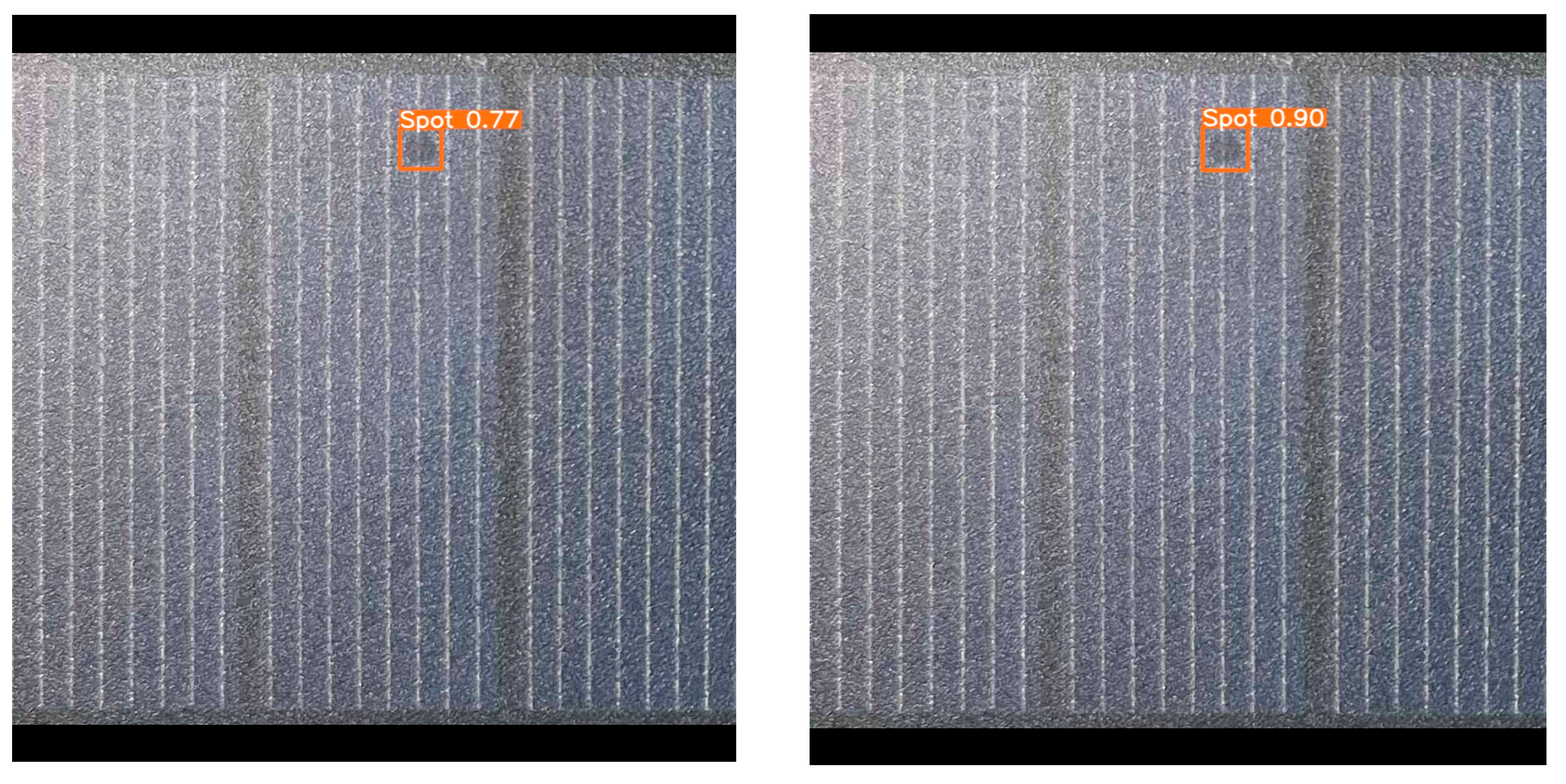
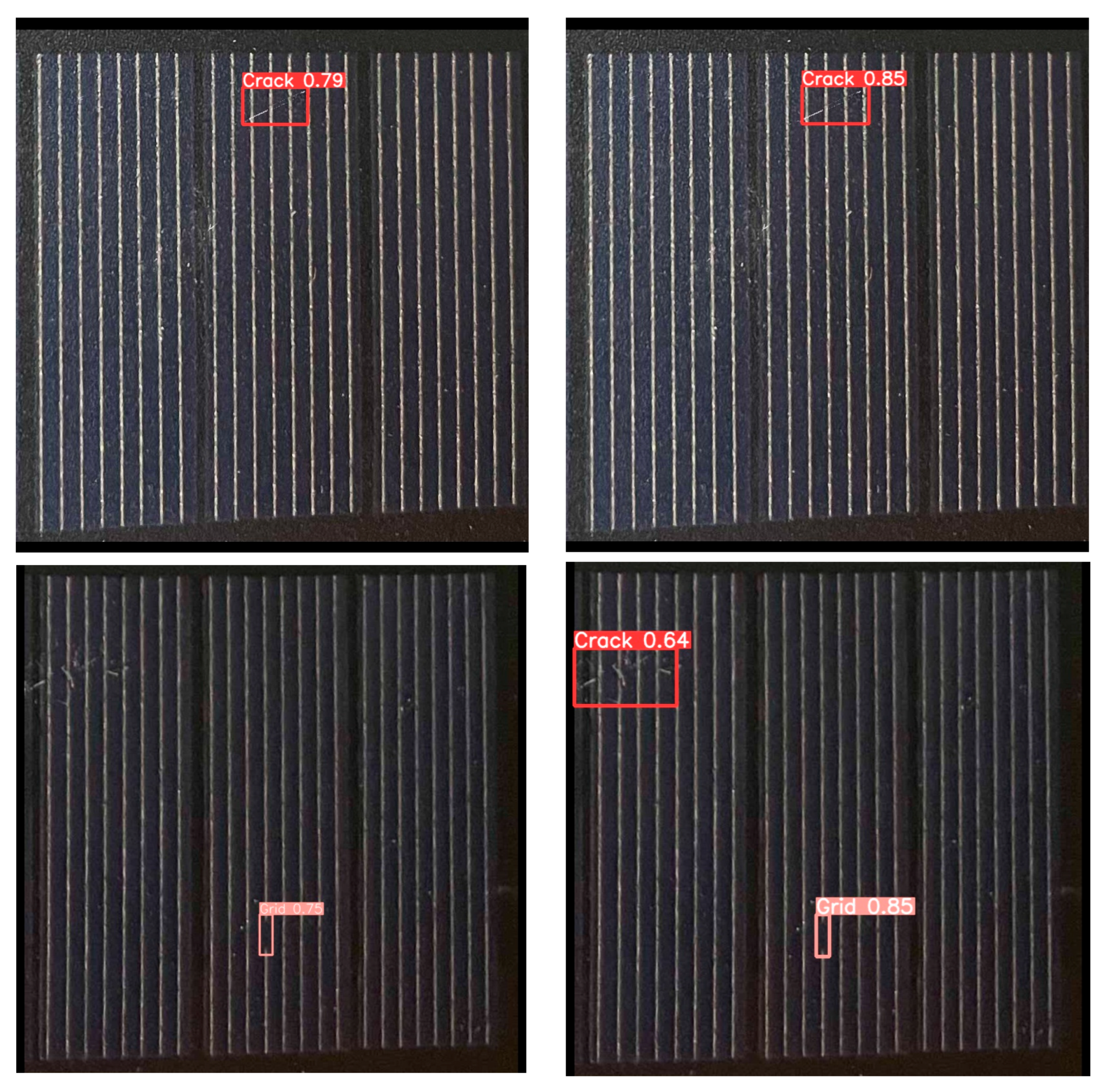
Our EER-DETR model has demonstrated excellent performance in detecting three types of defects, and the verification result is shown in Figure 6. Among them, the Precision rate for the spot is as high as 0.943, while the rates for crack and grid reach 0.891 and 0.882, respectively, indicating that the detection results are highly reliable, with an extremely low false detection rate. At the same time, the model also has strong Recall capabilities. The Recall rates for the three types of defects all exceed 0.85, proving that the model can effectively capture the vast majority of defects and significantly reduce the risk of missed detections. Under the conventional IoU threshold (0.5), the mAP50 for the grid and spot both exceed 0.9, and cracks are close to this level. This demonstrates the model’s balanced advantages in detection accuracy and coverage. The model maintains stable performance for different types of defects, verifying its practicality and generalization ability in complex industrial quality inspection scenarios. In summary, the EER-DETR model shows high accuracy, strong robustness, and comprehensiveness in detecting defects on photovoltaic panels, providing efficient and reliable technical support for industrial automated quality inspection.

Table 1. Test results for three defect detection types.

	Precision	Recall	mAP50	mAP50-90
Crack	0.891	0.855	0.864	0.461
Grid	0.882	0.862	0.914	0.442
Spot	0.943	0.897	0.938	0.451

presents the detection results for three different types of defects.

4.4.2. Comparative Experiments

From

Table 2. Comparison with the original model.

	Precision	Recall	mAP50	mAP50-90	Parameters	GFLOPs
RT-DETR	0.893	0.841	0.886	0.456	19,875,612	56.9
EER-DETR	0.916	0.872	0.905	0.458	17,941,933	48.6

, we can observe that EER-DETR outperforms the original model RT-DETR in multiple key indicators. In terms of Precision, EER-DETR achieved 0.916, while RT-DETR only reached 0.893, indicating that EER-DETR is more accurate in identifying targets and can more effectively reduce false alarms. In terms of Recall, EER-DETR also demonstrated an advantage, reaching 0.872, while RT-DETR was 0.841. This suggests that EER-DETR is more comprehensive in detecting targets and can more effectively reduce missed detections. In terms of mAP50 (mean average precision at 50%) and mAP50-90 (mean average precision at different IoU thresholds), EER-DETR also performed well, reaching 0.905 and 0.458, respectively, while RT-DETR was 0.886 and 0.456, respectively. Compared to the original model, this indicates an improvement of 1.9%. This shows that EER-DETR has superior comprehensive performance across different detection difficulties. Additionally, EER-DETR also demonstrated advantages in terms of parameter quantity and computational complexity. The parameter quantity of EER-DETR is 17,941,933, while that of RT-DETR is 19,875,612. The computational complexity (GFLOPs) of EER-DETR is 48.6, while that of RT-DETR is 56.9. This indicates that EER-DETR maintains high performance while having better computational efficiency and model lightweight characteristics. Figure 7 shows a comparison chart of the detection performance between EER-DETR and RT-DETR. It can be seen that the performance of our model has improved significantly.

To verify the stability of the model performance and the reliability of the improvements, five independent experiments were conducted on RT-DETR and EER-DETR, with the same data division and training configuration used in each experiment. The stability of the evaluation metrics was assessed by calculating the mean and standard deviation, and the paired t-test was used to verify whether the performance difference between the improved model and the original model was statistically significant (significance level α = 0.05).

The data in the table represent the mean values of five independent experiments, with standard deviations as follows: Precision (RT-DETR: ±0.008, EER-DETR: ±0.006); Recall (RT-DETR: ±0.009, EER-DETR: ±0.007); mAP50 (RT-DETR: ±0.007, EER-DETR: ±0.005). Paired t-test shows that EER-DETR is significantly superior to RT-DETR in Precision (t = 4.21, p < 0.05), Recall (t = 3.12, p < 0.05), and mAP50 (t = 5.12, p < 0.01).

We also compared EER-DETR with the classic YOLO series models. From

Table 3. Comparison with classical algorithms.

	Precision	Recall	mAP50	mAP50-90
Yolov5	0.891	0.865	0.888	0.446
Yolov7	0.862	0.743	0.775	0.366
Yolov8	0.879	0.776	0.856	0.453
Yolov9	0.903	0.868	0.902	0.484
Yolov10	0.851	0.795	0.848	0.445
Yolov11	0.871	0.821	0.875	0.463
EER-DETR	0.921	0.872	0.905	0.458

, we can see that EER-DETR demonstrated significant advantages in multiple indicators such as Precision, Recall, mAP50, and mAP50-90. In terms of Precision, EER-DETR reached 0.909; this indicates that EER-DETR has higher accuracy in target recognition. In terms of Recall, EER-DETR reached 0.872, while the best-performing model in the YOLO series, YOLOv5, was 0.865. This shows that EER-DETR has better comprehensiveness in target detection. In terms of mAP50 and mAP50-90, EER-DETR reached 0.905 and 0.458, respectively, while the best-performing model in the YOLO series, YOLOv5, reached 0.888 and 0.446, respectively. This indicates that EER-DETR has superior comprehensive performance under different detection difficulties. In contrast, the YOLO series models have shortcomings in some aspects. For example, YOLOv7 performed poorly in Precision and Recall, with 0.862 and 0.743, respectively, indicating that its accuracy and comprehensiveness in target recognition need to be improved. YOLOv10 also performed poorly in Precision and Recall, with 0.851 and 0.795, respectively, indicating that its performance in target detection needs to be enhanced.

As shown in

Table 4. Comparative experiments with different main structures replaced.

	Precision	Recall	mAP50	mAP50-90	Parameters	GFLOPs
SwinTransformer	0.894	0.839	0.886	0.441	36,319,810	97.0
VanillaNet	0.871	0.842	0.861	0.440	21,716,360	66.8
StarNet	0.855	0.827	0.835	0.436	11,994,248	31.8
ConvNextV2	0.862	0.831	0.841	0.444	12,306,808	31.9
EER-DETR	0.916	0.872	0.905	0.458	17,941,933	48.6

and

Table 5. Comparative experiments on replacing different encoder networks.

	Precision	Recall	mAP50	mAP50-90	Parameters	GFLOPs
SlimNeck	0.871	0.838	0.863	0.446	19,304,872	53.3
MAFPN	0.878	0.847	0.871	0.447	22,932,584	56.3
BIFPN	0.894	0.853	0.882	0.456	20,306,612	64.3
EER-DETR	0.916	0.872	0.905	0.458	17,941,933	48.6

, we tested the performance of various models on the photovoltaic panel defect dataset. However, in general, none of them outperformed our designed EER-DETR model.

Firstly, regarding different backbone structures, after improving RT-DETR with SwinTransformer, although it has higher parameters and computational complexity, it still performs reasonably well in Precision, Recall, mAP50, and mAP50-90 indicators. This indicates that it has certain advantages in feature extraction and object detection. However, compared with EER-DETR, SwinTransformer is slightly inferior in these indicators, especially in Precision and mAP50. EER-DETR achieved 0.909 and 0.905, respectively, while SwinTransformer only reached 0.864 and 0.852. This shows that EER-DETR is more accurate and has better detection performance. Models such as VanillaNet, StarNet, and ConvNextV2, which are improved models, have relatively lower parameters and computational complexity, but they still have a gap compared to EER-DETR in Precision, Recall, mAP50, and mAP50-90 indicators. Although VanillaNet is slightly higher than SwinTransformer in Precision and mAP50, it does not show obvious advantages in other indicators. This indicates that VanillaNet may have certain potential from some aspects, but its overall performance still needs further optimization.

Improvements and comparisons on different structures of the neck part were also made. After improving RT-DETR with SlimNeck, its parameters were reduced and the computational complexity was lower. However, there is still a gap in terms of the Precision, Recall, mAP50 and mAP50-90 indicators compared with EER-DETR. Using mAP for comparison, EER-DETR increased by 4.2% compared with SlimNeck and by 3.4% and 2.3%, respectively, compared with MAFPN and BIFPN. Meanwhile, our model has the lowest parameter quantity. It can be clearly seen from Figure 8 that EER-DETR has obvious advantages over the other models:

In conclusion, EER-DETR performs well in the Precision, Recall, mAP50, and mAP50-90 indicators and has relatively lower parameters and computational complexity. This indicates that EER-DETR has significant advantages in accuracy and detection performance and has high practicality and operability in actual applications. In contrast, other models have shortcomings in certain aspects. For instance, their recognition accuracy and detection comprehensiveness need to be improved, and their computational complexity and model lightweighting also require optimization. Therefore, the EER-DETR model has better performance and broader application prospects in practical applications.

4.4.3. Ablation Experiments

From

Table 6. The results of the ablation experiment.

RT-DETR	RepaNet	EHFPN	EUCB	mAP50	Parameters	GFLOPs
√				0.886	19,875,612	56.9
√	√			0.902	19,875,612	56.9
√		√		0.871	17,821,836	47.5
√			√	0.901	20,189,856	57.7
√	√	√		0.899	17,821,836	47.5
√	√	√	√	0.905	17,941,933	48.6

, it can be seen that, first, in the original RT-DETR model, mAP50 reached 0.886, with a parameter quantity of 19,875,612 and GFLOPs of 56.9. This indicates that the RT-DETR module itself already has a relatively high detection capability, but there is still room for improvement. When we improved RepaNet based on RT-DETR, the model’s mAP50 increased to 0.902, with the parameter quantity remaining unchanged and GFLOPs also remaining at 56.9. This shows that the RepaNet module significantly improves the detection performance of the model without increasing computational resources. Further, when the EHFPN module was added to RT-DETR, the model’s mAP50 slightly decreased to 0.871, but the parameter quantity was reduced to 17,821,836 and GFLOPs decreased to 47.5. This indicates that the EHFPN module reduces the computational resource requirements of the model to a certain extent, but the improvement in detection performance is limited. The EHFPN module reduces the parameter quantity and computational cost through a more efficient feature pyramid network design but may not be as good as RepaNet in feature extraction and fusion. When the EUCB module was added to RT-DETR, the model’s mAP50 increased to 0.901, the parameter quantity increased to 20,189,856, and GFLOPs increased to 57.7. This shows that the EUCB module further improves the detection performance of the model by increasing computational resources, enhancing the model’s ability to locate and classify targets. When RepaNet and EHFPN were added to RT-DETR simultaneously, the model’s mAP50 reached 0.899, the parameter quantity remained at 17,821,836, and GFLOPs remained at 47.5. This indicates that the combination of the RepaNet and EHFPN modules can still maintain high detection performance while reducing computational resources. The RepaNet module optimizes feature extraction and fusion, while the EHFPN module reduces the parameter quantity and computational cost through a more efficient feature pyramid network design. Finally, when the RepaNet, EHFPN, and EUCB modules are used simultaneously, our EER-DETR model is formed. The model’s mAP50 reached 0.905, the parameter quantity was reduced by 9.7% compared to the original RT-DETR model, and GFLOPs were significantly reduced. In conclusion, by gradually adding RepaNet, EHFPN, and EUCB modules, the detection performance of the model was significantly improved, and computational resource requirements were also optimized. This proves that our EER-DETR model achieved high accuracy and lightweight efficiency.

4.5. The Deployment on the NVIDIA Jetson Nano Platform

In practical applications, the real-time object detection capability of edge devices holds significant importance. This study deploys the improved EER-DETR model on the NVIDIA Jetson Nano platform, which is equipped with a quad-core Cortex-A57 CPU and a 128-core Volta architecture GPU and is suitable for edge computing scenarios. As shown in the

Table 7. The deployment on the NVIDIA Jetson Nano platform.

	Resolution	FPS	VRAM Usage (MB)	Power Consumption
RT-DETR	640 × 640	42.8	746	7.8
EER-DETR	640 × 640	36.5	599	6.9

, compared with the original RT-DETR, EER-DETR has significant improvements in indicators such as FPS and memory usage. These data indicate that EER-DETR not only enhances detection accuracy but also reduces model complexity, making it more suitable for resource-constrained edge devices. Deploying EER-DETR on Jetson Nano provides a better solution for real-time object detection in edge scenarios, achieving a better balance between accuracy and efficiency through specific data support.

4.6. The Test Conducted on the EER-DETR Model on the PVEL-AD Dataset

As shown in

Table 8. The test on the PVEL-AD dataset.

	Precision	Recall	mAP50	mAP50-90	Parameters	GFLOPs
RT-DETR	0.893	0.842	0.885	0.453	19,908,612	57.0
EER-DETR	0.915	0.868	0.901	0.457	17,987,586	48.7

, We tested our model on 9842 image pairs extracted from the PVEL-AD dataset. The results showed that, compared with the original RT-DETR model, the mAP50 of our model increased by 1.6% and the number of parameters decreased by 9.6%. The results indicate that our model is universal across different datasets for photovoltaic panel defect detection and achieves the goal of integrating high accuracy and lightweight.

5. Discussion and Conclusions

To significantly enhance the accuracy and real-time performance of photovoltaic panel defect detection, thereby providing strong technical support for the intelligent operation and maintenance of photovoltaic systems, this study proposes an improved photovoltaic panel defect detection method, EER-DETR, based on RT-DETR. Through in-depth experimental verification of this algorithm, the results show that the designed EER-DETR model exhibits excellent performance in photovoltaic panel defect detection, achieving a significant improvement in detection accuracy, while significantly reducing the computational cost. The EER-DETR algorithm adds a structural re-parameterization module, WDBB, to form a new feature extraction network, RepaNet and designs an efficient multi-scale convolution module and global heterogeneous kernel selection mechanism, EHFPN, to reduce computational overhead; introducing EUCB to optimize the upsampling process not only retains more details when improving image resolution but also enables the network to effectively learn small target features at low resolutions, thereby reducing the problem of missed detections and improving the accuracy and robustness of photovoltaic panel defect detection. This optimization makes the algorithm more stable and efficient in practical applications, especially in the defect detection tasks of large-scale photovoltaic power stations, where it demonstrates stronger adaptability compared to traditional methods.

However, this study still has certain limitations. Although data augmentation strategies were employed, in extremely complex environmental conditions (such as extreme lighting), the model’s detection accuracy for some minor defects may decline, and there is a risk of overfitting. Through qualitative analysis of the detection results, it was found that in some cases, when the light is uneven or the edge defect features are blurry, the model may have false detections or missed detections. For example, when the scratch defect is too similar to the texture of the panel itself, the model has difficulty accurately distinguishing them, resulting in detection errors. There are also deficiencies in the detection of some internal issues. These situations indicate that the model’s robustness in handling complex visual information still needs to be improved.

EER-DETR as an innovative method for detecting defects in photovoltaic panels, not only providing a new solution for intelligent operation and maintenance from a theoretical perspective but also demonstrating strong application potential in practice, indicating its broad application prospects in the future photovoltaic industry. Looking to the future, it is recommended to conduct in-depth research in the following directions: firstly, expand the range of detectable defects to include more rare defect types, and enhance the model’s generalization ability; secondly, integrate multi-spectral data and utilize the feature information under different spectral conditions to improve the ability to identify complex defects; finally, further optimize the domain adaptation algorithm to ensure that the model maintains stable and efficient detection performance in different environments and scenarios, promoting the continuous progress of photovoltaic panel defect detection technology.

References

1. Green, M.A.; Dunlop, E.D.; Yoshita, M.; Kopidakis, N.; Bothe, K.; Siefer, G.; Hao, X.; Jiang, J.Y. Solar cell efficiency tables (version 56). Prog. Photovolt. Res. Appl. 2020, 28, 629–638. [Google Scholar] [CrossRef]
2. Polly, S.J.; Dann, M.; Fedorenko, A.; Hubbard, S.; Landi, B.; Schauerman, C.; Ganter, M.; Raffaelle, R. Development of a nano-enabled space power system. In Proceedings of the 7th World Conference on Photovoltaic Energy Conversion (IEEE), Waikoloa, HI, USA, 10–15 June 2018; pp. 3389–3391. [Google Scholar]
3. Sharma, V.; Chandel, S.S. Performance and degradation analysis for long term reliability of solar photovoltaic systems: A review. Renew. Sustain. Energy Rev. 2013, 27, 753–767. [Google Scholar] [CrossRef]
4. Schmidt, M.; Braunger, D.; Schaffler, R.; Schock, H.W.; Rau, U. Influence of damp heat on the electrical properties of Cu (in,Ga) Se2 solar cells. Thin Solid Film. 2000, 361, 283–287. [Google Scholar] [CrossRef]
5. Banda, P.; Barnard, L. A deep learning approach to photovoltaic cell defect classification. In Proceedings of the Annual Conference of the South African Institute of Computer Scientists and Information Technologists on (SAICSIT), Port Elizabeth, South Africa, 26–28 September 2018; pp. 215–221. [Google Scholar]
6. Wilson, D.R.; Martinez, T.R. The general inefficiency of batch training for gradient descent learning. Neural Netw. 2003, 16, 1429–1451. [Google Scholar]
7. Memon, S.A.; Javed, Q.; Kim, W.G.; Mahmood, Z.; Khan, U.; Shahzad, M. A Machine-Learning-Based Robust Classification Method for PV Panel Faults. Sensors 2022, 22, 8515. [Google Scholar] [CrossRef] [PubMed] [PubMed Central]
8. Xie, H.; Yuan, B.; Hu, C.; Gao, Y.; Wang, F.; Wang, C.; Wang, Y.; Chu, P. ST-YOLO: A defect detection method for photovoltaic modules based on infrared thermal imaging and machine vision technology. PLoS ONE 2024, 19, e0310742. [Google Scholar] [CrossRef] [PubMed] [PubMed Central]
9. Carion, N.; Massa, F.; Synnaeve, G.; Usunier, N.; Kirillov, A.; Zagoruyko, S. End-to-End Object Detection with Transformers. arXiv 2020, arXiv:abs/2005.12872. [Google Scholar]
10. Li, L. Object Detection Based on K-Nearest Neighbor Contour Fragment Group. Sci. Technol. Inf. 2014, 66, 2011–2032. [Google Scholar]
11. Bartler, A.; Mauch, L.; Yang, B.; Reuter, M.; Stoicescu, L. Automated Detection of Solar Cell Defects with Deep Learning. In Proceedings of the 26th European Signal Processing Conference (EUSIPCO), Rome, Italy, 3–8 September; pp. 2035–2039.
12. Tang, W.; Yang, Q.; Xiong, K.; Yan, W. Deep learning based automatic defect identification of photovoltaic module using electroluminescence images. Sol. Energy 2020, 201, 453–460. [Google Scholar] [CrossRef]
13. Chen, X.; Karin, T.; Jain, A. Multiyear Study of Crack-Induced Degradation in Fielded Photovoltaic Modules. Sol. Energy 2022, 242, 20–29. [Google Scholar]
14. Hijjawi, U.; Lakshminarayana, S.; Xu, T.; Piero Malfense Fierro, G.; Rahman, M. A review of automated solar photovoltaic defect detection systems: Approaches, challenges, and future orientations. Sol. Energy 2023, 266, 112186. [Google Scholar] [CrossRef]
15. Wang, Y.; Guo, J.; Qi, Y.; Liu, X.; Han, J.; Zhang, J.; Zhang, Z.; Lian, J.; Yin, X. Research Progress on Deep Learning Based Defect Detection Technology for Solar Panels. EAI Endorsed Trans. Energy Web 2024, 11. [Google Scholar] [CrossRef]
16. Redmon, J.; Divvala, S.K.; Girshick, R.B.; Farhadi, A. You Only Look Once: Unified, Real-Time Object Detection. In Proceedings of the 2016 IEEE Conference on Computer Vision and Pattern Recognition (CVPR), Las Vegas, NV, USA, 27–30 June 2016; pp. 779–788. [Google Scholar]
17. Kong, S.; Xu, Z.; Lin, X.; Zhang, C.; Jiang, G.; Zhang, C.; Wang, K. Infrared Thermal Imaging Defect Detection for Photovoltaic Modules Based on Improved YOLO v5 Algorithm. Infrared Technol. 2023, 45, 974–981. [Google Scholar]
18. Wang, Y.; Zhao, J.; Yan, Y.; Zhao, Z.; Hu, X. Pushing the Boundaries of Solar Panel Inspection: Elevated Defect Detection with YOLOv7-GX Technology. Electronics 2024, 13, 1467. [Google Scholar] [CrossRef]
19. Jin, L.; Shi, L.; Liu, K.; Zhong, M.; Pang, Y. Real-Time Fault Diagnosis of Photovoltaic Modules for Integrated Energy Systems Based on YOLOv7. In Sixth International Conference on Computer Information Science and Application Technology (CISAT 2023), Hangyou, China, 26–28 May 2023; Jia, S., Dong, H., Eds.; SPIE: Bellingham, WA, USA, 2023; p. 197. [Google Scholar] [CrossRef]
20. Wang, Y.; Zhang, Z.; Zhang, J.; Han, J.; Lian, J.; Qi, Y.; Liu, X.; Guo, J.; Yin, X. Research on Surface Defect Detection Method of Photovoltaic Power Generation Panels—Comparative Analysis of Detecting Model Accuracy. EAI Endorsed Trans. Energy 2024, 11, 1. [Google Scholar] [CrossRef]
21. Dosovitskiy, A.; Beyer, L.; Kolesnikov, A.; Weissenborn, D.; Zhai, X.; Unterthiner, T.; Dehghani, M.; Minderer, M.; Heigold, G.; Gelly, S. An image is worth 16x16 words: Transformers for image recognition at scale. arXiv 2020, arXiv:2010.11929. [Google Scholar]
22. Carion, N.; Massa, F.; Synnaeve, G.; Usunier, N.; Kirillov, A.; Zagoruyko, S. End-to-end object detection with transformers. In Proceedings of the European Conference on Computer Vision, Glasgow, UK, 23–28 August 2020; pp. 213–229. [Google Scholar]
23. Zhu, X.; Su, W.; Lu, L.; Li, B.; Wang, X.; Dai, J. Deformable detr: Deformable transformers for end-to-end object detection. arXiv 2020, arXiv:2010.04159. [Google Scholar]
24. Yao, Z.; Ai, J.; Li, B.; Zhang, C. Efficient detr: Improving end-to-end object detector with dense prior. arXiv 2021, arXiv:2104.01318. [Google Scholar]
25. Zhao, Y.; Lv, W.; Xu, S.; Wei, J.; Wang, G.; Dang, Q.; Liu, Y.; Chen, J. Detrs beat yolos on real-time object detection. arXiv 2023, arXiv:2304.08069. [Google Scholar]
26. Wan, D.; Lu, R.; Hu, B.; Yin, J.; Shen, S.; Xu, T.; Lang, X. YOLO-MIF: Improved YOLOv8 with Multi-Information fusion for object detection in Gray-Scale images. Adv. Eng. Inform. 2024, 62, 102709. [Google Scholar] [CrossRef]
27. Ding, X.; Ding, G. Diverse Branch Block: Building a Convolution as an Inception-like Unit. arXiv 2021, arXiv:2103.13425. [Google Scholar]
28. Zhigang, S.; Xiang, Y.; Bing, H.; Jingtang, H.; Xinyi, Z. A Real Time Drone RF Signal Detection Method Under Low SNR Condition. J. Signal Process. 2023, 39, 919–928. [Google Scholar] [CrossRef]
29. Liu, Z.; Sun, C.; Wang, X. DST-DETR: Image Dehazing RT-DETR for Safety Helmet Detection in Foggy Weather. Sensors 2024, 24, 4628. [Google Scholar] [CrossRef] [PubMed]
30. Tan, M.; Pang, R.; Le, Q.V. Efffcientdet: Scalable and efffcient object detection. In Proceedings of the Conference on Computer Vision and Pattern Recognition (IEEE/CVF), Seattle, WA, USA, 13–19 June 2020; pp. 10781–10790. [Google Scholar]
31. Zhang, L.; Lyu, C.; Chen, Z.; Li, S.; Xia, B. Semantic Coarse-to-Fine Granularity Learning for Two-Stage Few-Shot Anomaly Detection. IJSWIS 2024, 20, 1–22. [Google Scholar] [CrossRef]
32. Rahman, M.M.; Munir, M.; Marculescu, R. EMCAD: Efficient Multi-Scale Convolutional Attention Decoding for Medical Image Segmentation. In Proceedings of the Conference on Computer Vision and Pattern Recognition (IEEE/CVF), Seattle, WA, USA, 21 June 2024; pp. 11769–11779. [Google Scholar]
33. Deng, J.; Chen, Z.; Chen, M.; Xu, L.; Yang, J.; Luo, Z.; Qin, P. Pneumonia App: A mobile application for efficient pediatric pneumonia diagnosis using explainable convolutional neural networks (CNN). arXiv 2024, arXiv:abs/2404.00549. [Google Scholar]
34. Su, B.; Zhou, Z.; Chen, H. PVEL-AD: A Large-Scale Open-World Dataset for Photovoltaic Cell Anomaly Detection. IEEE Trans. Ind. Inform. 2023, 19, 404–413. [Google Scholar] [CrossRef]
Figure 1. RT-DETR network structure diagram.
Applsci 15 06217 g001
Figure 2. EER-DETR network structure diagram.
Applsci 15 06217 g002
Figure 3. (a) The original branch of WDBB, (b) the K × K convolutional branch after unit transformation.
Applsci 15 06217 g003
Figure 4. Feature extraction network design: (a) FPN, (b) PANet, (c) NAS-FPN, and (d) BiFPN.
Applsci 15 06217 g004
Figure 5. EUCB.
Applsci 15 06217 g005
Figure 6. The feature graphs of different layers in the training process.
Applsci 15 06217 g006
Figure 7. The comparison chart of detection performance between EER-DETR and RT-DETR.
Applsci 15 06217 g007aApplsci 15 06217 g007b
Figure 8. Scatter plots comparing different models.
Applsci 15 06217 g008