Physics-Informed Neural Networks-Based Wide-Range Parameter Displacement Inference for Euler–Bernoulli Beams on Foundations Under a Moving Load Using Sparse Local Measurements

Abstract

This study develops a novel physics-informed neural network (PINN) framework for predicting steady-state dynamic responses of infinite Euler–Bernoulli (E–B) beams on foundations under moving loads. By combining localized PINN modeling with transfer learning techniques, our approach achieves high-fidelity predictions across broad parameter ranges while significantly reducing data requirements. Numerical results show that the method maintains accuracy with less than half the training data of conventional PINN models (15 target domains) and remains effective with just four domains for approximate solutions. Key findings demonstrate that optimal spatial distribution—rather than quantity—of target domains ensures robustness against noise and parameter variations. The framework advances data-efficient surrogate modeling, enabling reliable predictions in data-scarce scenarios with applications to complex engineering systems where experimental data are limited.

1. Introduction

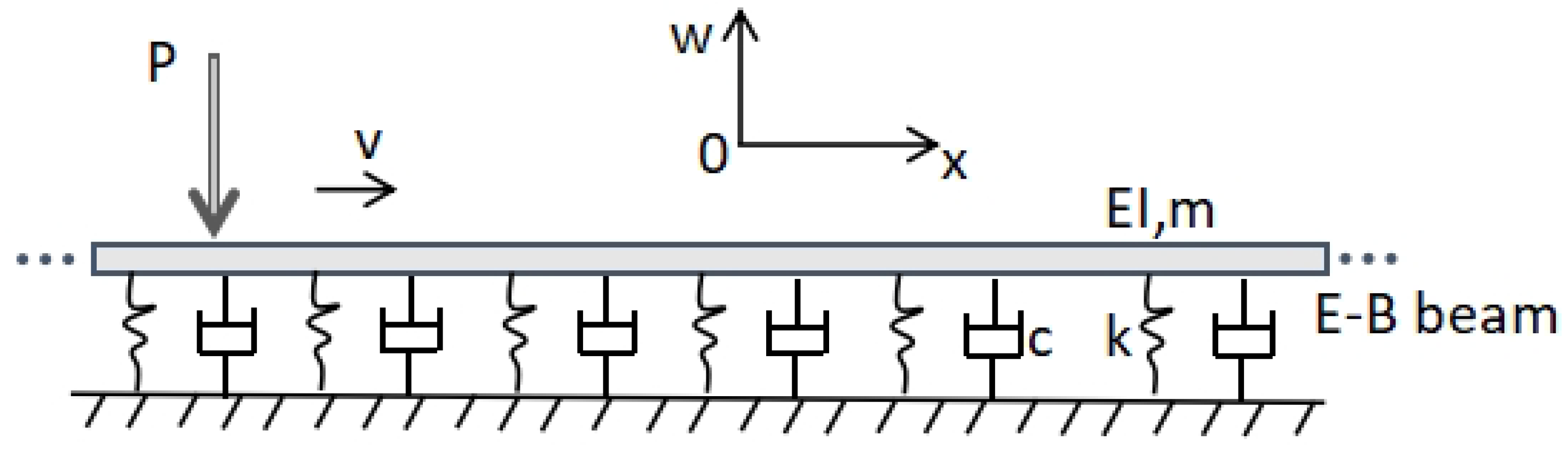
The dynamic response calculation of a foundation beam under moving loads represents a highly complex mechanical issue that integrates knowledge and techniques from multiple disciplines. Addressing this problem not only deepens our understanding of dynamic responses in practical engineering scenarios but also offers theoretical and technical support to ensure structural safety and reliability [1,2]. The solutions to this problem typically involve analytical and numerical methods. Analytical methods necessitate the formulation of mathematical models, followed by the application of integral transforms (e.g., Laplace, Fourier) to solve the governing equations. This process yields closed-form solutions that offer clear insights into how different parameters influence dynamic responses [3,4]. However, these methods are generally restricted to idealized models and specific loading conditions. In contrast, numerical methods, which often utilize the finite element method (FEM), are capable of tackling complex real-world engineering problems. They can manage irregular geometries, complex boundary conditions, and multiphysics couplings but demand significant computational resources [5]. Furthermore, a single finite element simulation can only provide the solution for a particular case. When variables such as material properties, structural models, or loading patterns change, remodeling and remeshing become necessary. This lack of adaptability renders finite element simulation inefficient for certain problems [6].

In recent years, deep learning (DL) techniques, celebrated for their remarkable fitting capabilities, have garnered significant attention in the analysis and prediction of dynamic responses induced by moving loads [7,8,9]. The effectiveness of these DL methods largely hinges on supervised training, where the model adjusts its parameters by calculating the error between predicted and true labels (loss function) and then uses backpropagation and optimizers (e.g., gradient descent) to minimize this error. Repeated iterations of this process enable the model to improve and achieve high accuracy on test data [10,11]. However, in practical applications, obtaining high-quality monitoring data is often fraught with difficulties [12]. As a result, accurately predicting the dynamic response of structures becomes extremely challenging when data are scarce or unavailable. Recently, physics-informed neural networks (PINNs), which combine scientific computing and machine learning, have shown considerable potential for solving partial differential equations (PDEs) in data-scarce scenarios [13,14,15]. Research on the application of PINNs to beam bending problems, particularly dynamic responses under moving loads, is still in its early stages. Kapoor et al. [16] explored single—and double—beam structures using PINNs based on Euler–Bernoulli (E–B) and Timoshenko theories. Their work proved PINNs’ effectiveness in solving forward and inverse problems in complex beam systems. In follow-up studies, by modeling moving loads with Gaussian functions, PINNs were used to calculate beam deflection and predict moving loads [17]. However, this method treated the moving load as a static load progressing across different positions, neglecting dynamic effects. Fallah and Aghdam [18] applied PINNs to study the bending, natural frequencies, and free vibrations of 3D functionally graded porous beams, analyzing how material distribution, elastic foundation, porosity factor, and porosity distribution type affect bending response and natural frequencies. However, their research focused only on the spatial conditions under external loads, ignoring complex spatiotemporal effects. Li et al. [19] approximated the Dirac function with a Gaussian function, introduced a Fourier embedding layer into PINNs’ deep neural network, and incorporated causal weights into the loss function to obtain beam dynamic responses under moving loads. When beam parameters are unknown, a physics- and data-driven PINN can determine the beam response with minimal monitored data. When the training data are incomplete, the performance of PINNs often surpasses that of existing data-driven DL networks [13].

Although PINN has demonstrated significant potential in addressing computational physics problems involving sparse, noisy, unstructured, and multi-fidelity data, they still encounter numerous challenges when it comes to structural vibration problems under moving loads. PINN can only serve as a solver for specific parameter domains. When it comes to predicting dynamic responses over a broad range of parameter domains, the stability of PINN is not satisfactory. Each minor adjustment to the model means that retraining is necessary, a limitation that undoubtedly increases computational costs and makes it inconvenient to apply to practical engineering [20]. Constructing PINN-based surrogate models is seen as a way to enhance prediction generalization across broad parameter spaces [21,22,23]. Traditional PINN-based surrogate models can make wide-ranging predictions across parameter spaces by dynamically combining input parameters. However, these models face three key practical limitations: First, they struggle with computational efficiency as more parameters are added. This “dimensionality problem” becomes especially serious in complex cases like tuning multiple hyperparameters together, modeling interacting physical systems, or simulating time-dependent processes. The computational load grows much faster than for simpler PINN models. Second, the models need large amounts of training data to work accurately. Their prediction quality depends heavily on having enough data points covering the parameter space. With too little data, errors become much larger at the edges of the parameter range. The problem gets worse for systems with multiple scales or sudden physical changes. Most importantly, to work across all possible parameter values, the models must simplify the underlying physics. They use less complex versions of the governing equations and are less strict about satisfying physical laws exactly. While this helps the models fit data overall, it leads to bigger mistakes when dealing with special cases like sharp boundaries or critical parameter values where the physics changes suddenly. These limitations reduce how much we can trust the models in realistic, complex situations.

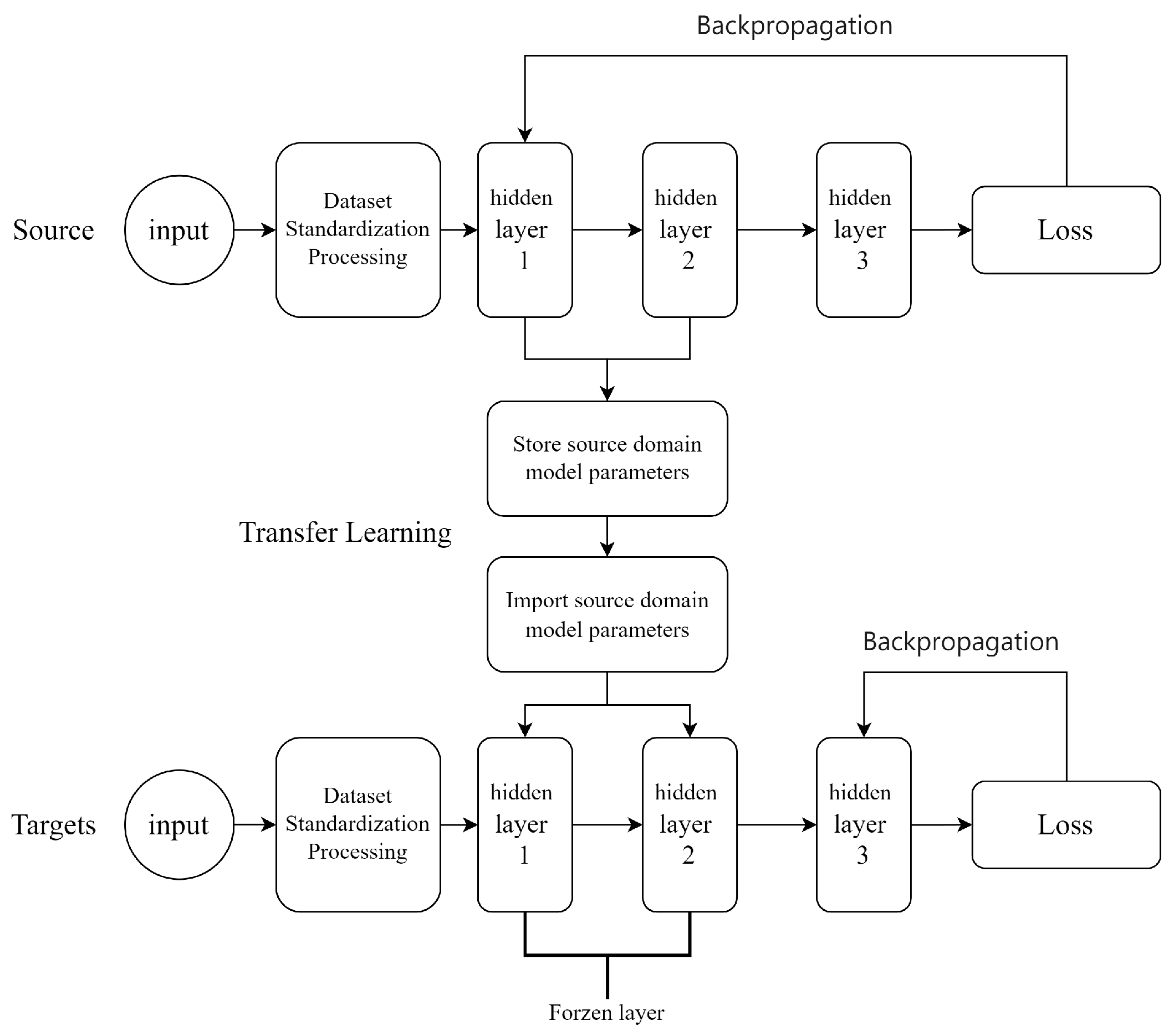
Based on the above considerations, our study addresses these challenges by developing a novel transfer learning [24,25]-enhanced PINN framework that strategically combines localized physical modeling with data-driven generalization. This hybrid approach enables accurate prediction of steady-state beam responses under moving loads across broad parameter ranges while significantly reducing the experimental or computational data needed for model training—a crucial advancement for practical engineering applications where comprehensive parameter testing is often infeasible. The proposed methodology begins by establishing local PINN models trained on displacement data obtained at strategically distributed points throughout the parameter space. These sampled points form the source domain, with their immediate adjacent regions designated as target domains. Leveraging transfer learning techniques, the initially trained source domain models undergo systematic refinement to achieve proper adaptation to each corresponding target domain. Ultimately, predictions generated by all localized PINN models across both source and target domains are integrated to construct a comprehensive PINN-based surrogate model capable of representing the system’s behavior across the full parameter spectrum. Transfer learning can significantly reduce the required input data volume for target domain tasks [26,27]. However, the transfer strategies employed in transfer learning can substantially impact the predictive performance of the resulting target domain models [28,29,30]. Current transfer strategies often rely heavily on experimental experience while lacking universal guiding principles. This paper provides relevant recommendations by examining how migration paths influence final prediction accuracy.

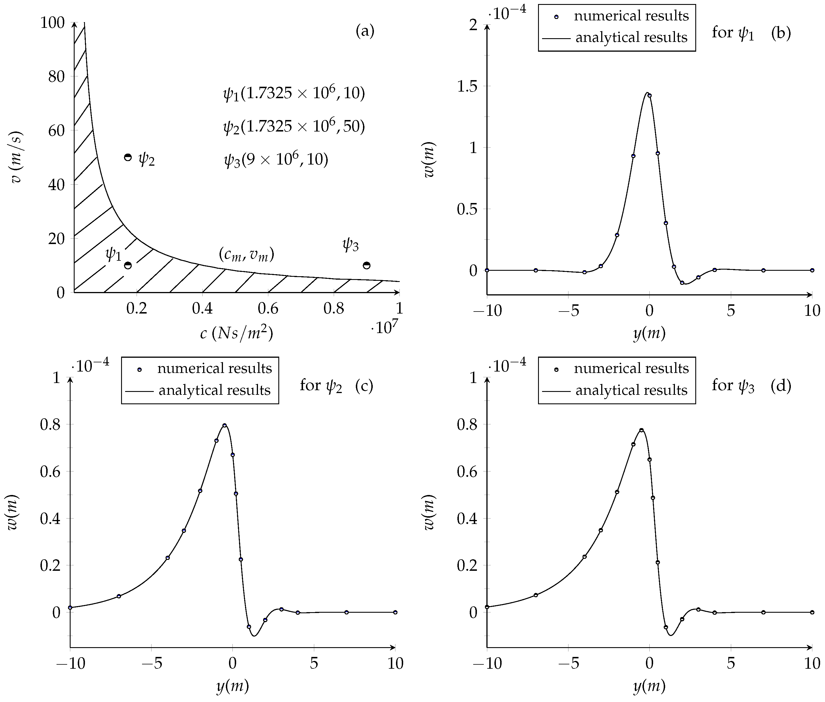
The remainder of this paper is organized as follows: In Section 2, an analytical solution is presented for the vibration problem of an infinite beam on a foundation subjected to a moving load. The analytical approach yields a limited dataset of displacement responses for the beam under prescribed parameter conditions. These displacement data are subsequently perturbed with noise to emulate sensor measurements. Additionally, the analytical solution is employed to generate response data across a broader range of arbitrary parameters, which serve as benchmark values for validating the surrogate model results in subsequent sections. In Section 3, three PINN models are developed to learn displacement data across various parameter conditions, aiming to identify the relationship between coordinates and beam displacement under specific parameters with limited measured data. In Section 4, transfer learning is utilized to adjust the weights of the initial PINN models for specific parameters. By leveraging the mapping capabilities of these PINN models, a large dataset of beam displacement responses is generated across several targeted regions within the parameter space. This dataset is then utilized in Section 5 to train a PINN-based surrogate model. Numerical examples show that the surrogate model accurately predicts beam displacement over a wide parameter range. A comparison between the prediction results of this study and those from traditional PINN-based surrogate models is presented in Section 6. Section 7 examines the impact of sensor measurement noise and transfer quantity and paths in transfer learning on the prediction accuracy of the surrogate model. The conclusions are presented in Section 8. For easy understanding, a list of symbols used in this paper along with their definitions is placed at the end of the text.

2. The Acquisition of Displacement Response Data for an Infinite Beam on a Foundation Subjected to a Moving Load

2.1. The Governing Equation

A schematic diagram of the vibration of an infinite E–B beam supported by a foundation under a moving load is shown in Figure 1. The governing equation that describes the dynamic behavior of the beam is provided below:

$$EI{\displaystyle \frac{{\partial }^{4}w}{\partial x^4}}+\rho A{\displaystyle \frac{{\partial }^{2}w}{\partial t^2}}+c{\displaystyle \frac{\partial w}{\partial t}}+kw=P\delta (x-vt),$$

(1)

where $w=w(x,t)$ represents the beam’s transverse deflection, with E as the modulus of elasticity and I as the second moment of area. $\rho$ stands for the beam material’s density, and A denotes the beam’s cross-sectional area. The foundation’s stiffness and damping coefficient are indicated by k and c, respectively. The moving load’s magnitude and velocity are represented by P and v, while $\delta \left(·\right)$ signifies the Dirac function. Since the beam is of infinite length, the boundary conditions can be expressed as

$$\underset{x\to \pm \infty }{lim}w(x,t)=0,\underset{x\to \pm \infty }{lim}{\displaystyle \frac{{\partial }^{j}w(x,t)}{\partial x^j}}=0,j=1,2,3,4.$$

(2)

The boundary conditions indicate that the slopes and curvatures of points far from the moving load tend to zero. To analyze the beam’s steady-state response, a new coordinate system can be introduced, fixed relative to the moving load, as follows:

$$y=x-vt.$$

(3)

From the differentiation chain rule, one has

$${\displaystyle \frac{{\partial }^{4}w}{\partial x^4}}={\displaystyle \frac{d^{4}w}{d{y}^4}},{\displaystyle \frac{\partial w}{\partial t}}=-v{\displaystyle \frac{dw}{dy}},{\displaystyle \frac{{\partial }^{2}w}{\partial t^2}}=v^2{\displaystyle \frac{d^{2}w}{d{y}^2}}.$$

(4)

Then Equation (1) can be converted into

$${\displaystyle \frac{{\mathrm{d}}^{4}w}{\mathrm{d}{y}^4}}+{\beta }_1{\displaystyle \frac{{\mathrm{d}}^{2}w}{\mathrm{d}{y}^2}}+{\beta }_2{\displaystyle \frac{\mathrm{d}w}{\mathrm{d}y}}+{\beta }_{3}w={\beta }_4\delta \left(y\right),$$

(5)

where

$${\beta }_1={\displaystyle \frac{\rho A{v}^2}{EI}},{\beta }_2=-{\displaystyle \frac{cv}{EI}},{\beta }_3={\displaystyle \frac{k}{EI}},{\beta }_4={\displaystyle \frac{P}{EI}}.$$

2.2. The Analytical Solution

We obtain the solution to Equation (5) by employing the Fourier transform, which is defined as follows:

$$\begin{array}{ccc}\hfill \widehat{w}\left(\xi \right)& =& {\int }_{-\infty }^{+\infty }w\left(y\right)e^{-i\xi y}dy,\hfill \\ \hfill w\left(y\right)& =& {\displaystyle \frac{1}{2\pi }}{\int }_{-\infty }^{+\infty }\widehat{w}\left(\xi \right)e^{i\xi y}d\xi .\hfill \end{array}$$

(6)

By applying the Fourier transform to Equation (5), we can derive the following result:

$$\begin{array}{c}\hfill \widehat{w}={\int }_{-\infty }^{+\infty }w\left(y\right)e^{-i\xi y}dy={\displaystyle \frac{{\beta }_4}{{\xi }^4-{\beta }_1{\xi }^2+i{\beta }_2\xi +{\beta }_3}}.\end{array}$$

(7)

To apply the residue theorem for calculating the inverse Fourier transform of the above equation, the root configuration of the denominator in Equation (7) must be determined. Let $f\left(\xi \right)$ denote the denominator in Equation (7), and $f_d\left(\xi \right)$ denote its derivative, as follows:

$$\begin{array}{cc}\hfill & f\left(\xi \right)={\xi }^4-{\beta }_1{\xi }^2+i{\beta }_2\xi +{\beta }_3,\hfill \\ \hfill & f_d\left(\xi \right)=4{\xi }^3-2{\beta }_1\xi +i{\beta }_2.\hfill \end{array}$$

(8)

To simplify the analysis, substituting $\xi =i\kappa$ into $f\left(\xi \right)$ gives

$$\begin{array}{c}\hfill g_1\left(\kappa \right)=f\left(i\kappa \right)={\kappa }^4+{\beta }_1{\kappa }^2-{\beta }_2\kappa +{\beta }_3.\end{array}$$

(9)

All coefficients of $g_1\left(\kappa \right)$ are real. If $g_1\left(\kappa \right)$ has a pair of complex roots $M_1\pm i{M}_2$, then $\mp M_2+i{M}_1$ must be two complex roots of $f\left(\xi \right)$. To further simplify the analysis for Equation (9), substituting $\kappa =\sqrt{{\beta }_1}\mu$ into Equation (9) transforms it into

$$g_2\left(\mu \right)=g_1\left(\sqrt{{\beta }_1}\mu \right)={\beta }_1^2({\mu }^4+{\mu }^2+{\gamma }_1\mu +{\gamma }_2)\equiv {\beta }_1^2{g}_3\left(\mu \right),$$

(10)

where ${\gamma }_1=-{\beta }_2{\beta }_1^{-{\displaystyle \frac{3}{2}}}$, ${\gamma }_2={\beta }_3{\beta }_1^{-2}$. Differentiating $g_3\left(\mu \right)$ with respect to $\mu$ yields

$$\begin{array}{cc}\hfill & g_{d1}\equiv {\displaystyle \frac{d{g}_3\left(\mu \right)}{d\mu }}=4({\mu }^3+{\displaystyle \frac{1}{2}}\mu +{\displaystyle \frac{{\gamma }_1}{4}}),\hfill \\ \hfill & g_{d2}\equiv {\displaystyle \frac{d^2{g}_3\left(\mu \right)}{d{\mu }^2}}=12{\mu }^2+2.\hfill \end{array}$$

(11)

From Cartan’s formula, the discriminant of the polynomial $g_{d1}$ can be determined as

$$\Delta ={\left({\displaystyle \frac{{\gamma }_1}{8}}\right)}^2+{\left({\displaystyle \frac{1}{6}}\right)}^3.$$

Evidently, $\Delta >0$ for any ${\gamma }_1$, so the polynomial $g_{d1}$ has one real root and a pair of conjugate complex roots. Suppose $\mu ={\mu }_0$ is the unique real root of $g_{d1}$, as follows:

$$g_{d1}\left({\mu }_0\right)={\mu }_0^3+{\displaystyle \frac{1}{2}}{\mu }_0+{\displaystyle \frac{{\gamma }_1}{4}}=0.$$

(12)

${\mu }_0$ can be explicitly written as

$${\mu }_0=-{\displaystyle \frac{1}{6}}\left(e_1\left({\gamma }_1\right)+e_2\left({\gamma }_1\right)\right).$$

(13)

where $e_1\left({\gamma }_1\right)=\sqrt[3]{27{\gamma }_1+3\sqrt{81{{\gamma }_1}^2+24}}$, $e_2\left({\gamma }_1\right)=\sqrt[3]{27{\gamma }_1-3\sqrt{81{{\gamma }_1}^2+24}}$.

It is straightforward to verify that ${\mu }_0<0$ from the equation above. Given that $g_{d2}>0$ for any $\mu$ (as per the second equation in Equation (11)), when $\mu <{\mu }_0$, $g_{d1}<0$, whereas when $\mu >{\mu }_0$, $g_{d_1}>0$. Consequently, the function $g_3\left(\mu \right)$ is strictly increasing (or decreasing) for $\mu >{\mu }_0$ (or $\mu <{\mu }_0$). Moreover, $g_3\left(\mu \right)$ attains its minimum value at $\mu ={\mu }_0$.

$$g_{{\mu }_0}\equiv g_3\left({\mu }_0\right)={\mu }_0^4+{\mu }_0^2+{\gamma }_1{\mu }_0+{\gamma }_2.$$

(14)

Substituting Equation (13) into Equation (14), one has

$$g_{{\mu }_0}=(-{\displaystyle \frac{1}{2}}{\mu }_0^2-{\displaystyle \frac{1}{4}}{\gamma }_1{\mu }_0)+{\mu }_0^2+{\gamma }_1{\mu }_0+{\gamma }_2={\displaystyle \frac{1}{2}}{\mu }_0^2+{\displaystyle \frac{3}{4}}{\gamma }_1{\mu }_0+{\gamma }_2.$$

(15)

The root configurations of the polynomial $g_3\left(\mu \right)$ can be expressed as follows:

$$\begin{array}{c}\hfill g_3\left(\mu \right)=\left\{\begin{array}{cc}[\mu -(d_1+i{d}_2)][\mu -(d_1-i{d}_2)](\mu -{\mu }_1)(\mu -{\mu }_2),\hfill & {g_{\mu }}_0<0,\hfill \\ [\mu -(d_3+i{d}_4)][\mu -(d_3-i{d}_4)]{(\mu -{\mu }_0)}^2,\hfill & {g_{\mu }}_0=0,\hfill \\ [\mu -(d_5+i{d}_6)][\mu -(d_5-i{d}_6)][\mu -(d_7+i{d}_8)][\mu -(d_7-i{d}_8)],\hfill & {g_{\mu }}_0>0,\hfill \end{array}\right.\end{array}$$

(16)

where $d_{1,\dots ,8},{\mu }_{1,2}\in R$. Moreover, $d_{1,\dots ,8}\ne 0$, ${\mu }_{1,2}\ne 0$ and ${\mu }_1<{\mu }_2$. The root configuration of the polynomial $f\left(\xi \right)$ can be written as

$$\begin{array}{c}\hfill f\left(\xi \right)=\left\{\begin{array}{cc}[\xi -(i{b}_1+b_2)][\xi -(i{b}_1-b_2)](\xi -i{c}_1)(\xi -i{c}_2),\hfill & {g_{\mu }}_0<0,\hfill \\ [\xi -(i{b}_3+b_4)][\xi -(i{b}_3-b_4)]{(\xi -i{c}_0)}^2,\hfill & {g_{\mu }}_0=0,\hfill \\ [\xi -(i{b}_5+b_6)][\xi -(i{b}_5+b_6)][\xi -(i{b}_7+b_8)][\xi -(-i{b}_7-b_8)],\hfill & {g_{\mu }}_0>0,\hfill \end{array}\right.\end{array}$$

(17)

where $b_i=\sqrt{{\beta }_1}{d}_i$, $i=1,2,\dots ,8$; $c_j=\sqrt{{\beta }_1}{\mu }_j$, $j=0,1,2$.

To compute the inverse Fourier transform of Equation (7) using the residue theorem, the signs of $b_{1,3,5,7}$ and $c_{1,2}$ must be determined. Based on the relationship between roots and coefficients in the first equation of Equation (16), the signs of $d_{1,3,5,7}$ and $c_{1,2}$ can be presented as

$$\left\{\begin{array}{cc}{b}_1>0,0>c_1>c_2,\hfill & {g_{\mu }}_0<0,\hfill \\ b_3>0,c_0<0,\hfill & {g_{\mu }}_0=0,\hfill \\ b_5>0,b_7<0,\hfill & {g_{\mu }}_0>0.\hfill \end{array}\right.$$

(18)

Substituting Equation (13) into Equation (15) yields

$$\begin{array}{c}\hfill {g_{\mu }}_0\left({\gamma }_1\right)={\displaystyle \frac{1}{72}}{(e_1\left({\gamma }_1\right)+e_2\left({\gamma }_1\right))}^2-{\displaystyle \frac{1}{8}}{\gamma }_1(e_1\left({\gamma }_1\right)+e_2\left({\gamma }_1\right))+{\gamma }_2.\end{array}$$

(19)

Taking the derivative of ${g_{\mu }}_0\left({\gamma }_1\right)$ with respect to ${\gamma }_1$ results in

$${g_{\mu }^{\prime }}_0\left({\gamma }_1\right)={\displaystyle \frac{1}{4}}({\displaystyle \frac{e_1\left({\gamma }_1\right)+e_2\left({\gamma }_1\right)}{9}}-{\displaystyle \frac{{\gamma }_1}{2}}){\displaystyle \frac{d(e_1\left({\gamma }_1\right)+e_2\left({\gamma }_1\right))}{d{\gamma }_1}}-{\displaystyle \frac{{\gamma }_1}{8}}(e_1\left({\gamma }_1\right)+e_2\left({\gamma }_1\right)).$$

(20)

It can be easily verified that ${g_{\mu }^{\prime }}_0\left({\gamma }_1\right)<0$ holds for any ${\gamma }_1>0$, indicating that ${g_{\mu }}_0$ decreases as ${\gamma }_1$ increases. Considering the definition of ${\gamma }_1$ in Equation (10), there must exist a unique velocity $v=v_m$ (where v is the velocity of the moving load) such that ${g_{\mu }}_0\left(v_m\right)=0$ for given mechanical and geometric properties of the beam and the moving load (with fixed values of c, k, m, and P). Moreover, ${g_{\mu }}_0\left(v\right)>0$ when $v>v_m$, and ${g_{\mu }}_0\left(v\right)<0$ when $v<v_m$. Therefore, Equations (17) and (18) can be rewritten as

$$f\left(\xi \right)=\left\{\begin{array}{c}[\xi -(i{b}_1+b_2)][\xi -(i{b}_1-b_2)](\xi -i{c}_1)(\xi -i{c}_2),v>v_m,\hfill \\ [\xi -(i{b}_3+b_4)][\xi -(i{b}_3-b_4)]{(\xi -i{c}_0)}^2,v=v_m,\hfill \\ [\xi -(i{b}_5+b_6)][\xi -(i{b}_5-b_6)][\xi -(i{b}_7+b_8)][\xi -(i{b}_7-b_8)],v<v_m,\hfill \end{array}\right.$$

$$and,\left\{\begin{array}{cc}{b}_1>0,0>c_1>c_2,\hfill & v>v_m,\hfill \\ b_3>0,c_0<0,\hfill & v=v_m,\hfill \\ b_5>0,b_7<0,\hfill & v<v_m,\hfill \end{array}\right.$$

(21)

where $v=v_m$ is the unique positive real root of the equation ${g_{\mu }}_0\left(v\right)=0$. Since the case $v=v_m$ is less meaningful, the following analysis focuses on $v>v_m$ and $v<v_m$. Applying the inverse Fourier transform to Equation (7) and using the residue theorem yields

$$w={\displaystyle \frac{1}{2\pi }}{\int }_{-\infty }^{+\infty }{\displaystyle \frac{{\beta }_4{e}^{i\xi y}}{{\xi }^4-{\beta }_1{\xi }^2+i{\beta }_2\xi +{\beta }_3}}d\xi =\left\{\begin{array}{cc}{W}_b,\hfill & y<0,\hfill \\ W_f,\hfill & y\ge 0,\hfill \end{array}\right.$$

(22)

where

$$W_b=\left\{\begin{array}{cc}{q}_1{e}^{-c_{1}y}+q_2{e}^{-c_{2}y},\hfill & v>v_m,\hfill \\ (q_3{e}^{-i{b}_{8}y}+q_4{e}^{i{b}_{8}y})e^{-b_{7}y},\hfill & v<v_m,\hfill \end{array}\right.$$

(23)

$$W_f=\left\{\begin{array}{cc}(q_5{e}^{-i{b}_{2}y}+q_6{e}^{i{b}_{2}y})e^{-b_{1}y},\hfill & v>v_m,\hfill \\ (q_7{e}^{-i{b}_{6}y}+q_8{e}^{i{b}_{6}y})e^{-b_{5}y},\hfill & v<v_m,\hfill \end{array}\right.$$

(24)

$$\begin{array}{cc}\hfill & q_1=-{\beta }_{4}i{\left[f_d\left(i{c}_1\right)\right]}^{-1},q_2=-{\beta }_{4}i{\left[f_d\left(i{c}_2\right)\right]}^{-1},q_3=-{\beta }_{4}i{\left[f_d(-b_8+i{b}_7)\right]}^{-1},\hfill \\ \hfill & q_4=-{\beta }_{4}i{\left[f_d(b_8+i{b}_7)\right]}^{-1},q_5={\beta }_{4}i{\left[f_d(-b_2+i{b}_1)\right]}^{-1},q_6={\beta }_{4}i{\left[f_d(b_2+i{b}_1)\right]}^{-1},\hfill \\ \hfill & q_7={\beta }_{4}i{\left[f_d(-b_6+i{b}_5)\right]}^{-1},q_8={\beta }_{4}i{\left[f_d(b_6+i{b}_5)\right]}^{-1},\hfill \end{array}$$

$f_d\left(·\right)$ is given by Equation (8).

2.3. Numerical Validation

In this subsection, we validate the correctness of w derived in Equations (22)–(24). The numerical simulations use the following mechanical and geometric properties [31]:

$$\begin{array}{cc}\hfill & E=210\left(\mathrm{GPa}\right),m=60.3665\left(\mathrm{kg}\right),I=30.55\times {10}^{-6}\left({\mathrm{m}}^4\right),\hfill \\ \hfill & k=35.03(\mathrm{MN}/{\mathrm{m}}^2),P=10\left(\mathrm{kN}\right).\hfill \end{array}$$

(25)

The velocity v of the moving load and the damping coefficient c are treated as key variables in the analysis. From Equation (19), the curves for $g_{{\mu }_0}(c,v)=0$ are plotted in Figure 2a, showing critical velocity $v_m$ and damping coefficient $c_m$. Three points, ${\psi }_{1,2,3}$, are marked in Figure 2a with the coordinates ${\psi }_1(1.7325\times {10}^6,10)$, ${\psi }_2(1.7325\times {10}^6,50)$, and ${\psi }_3(9\times {10}^6,10)$. Solving the first equation in Equation (8) for these points yields

$$\begin{array}{c}\hfill \xi =\left\{\begin{array}{cc}\pm 1.3500+1.0990i,\pm 0.7707-1.0990i,\hfill & forpoint{\psi }_1,\hfill \\ \pm 2.0756+1.3152i,-0.4067i,-2.2236i,\hfill & forpoint{\psi }_2,\hfill \\ \pm 2.0988+1.3278i,-0.3909i,-2.2647i,\hfill & forpoint{\psi }_3.\hfill \end{array}\right.\end{array}$$

(26)

From Equations (23) and (24), we have

$$\begin{array}{c}\hfill W_b=\left\{\begin{array}{cc}{10}^{-4}\times [1.4216cos\left(0.7707y\right)-2.5427sin\left(0.7707y\right)]e^{1.0990y},\hfill & forpoint{\psi }_1,\hfill \\ {10}^{-4}\times [1.1796e^{0.4067y}-0.5097e^{2.2236y}],\hfill & forpoint{\psi }_2,\hfill \\ {10}^{-4}\times [1.1304e^{0.3909y}-0.4805e^{2.2647y}],\hfill & forpoint{\psi }_3.\hfill \end{array}\right.\end{array}$$

(27)

$$\begin{array}{c}\hfill W_f=\left\{\begin{array}{cc}{10}^{-4}\times [1.4216cos\left(1.3500y\right)+0.863sin\left(1.3500y\right)]e^{-1.0990y},\hfill & forpoint{\psi }_1,\hfill \\ {10}^{-5}\times [6.6987cos\left(2.0756y\right)+1.0952sin\left(2.0756y\right)]e^{-1.3152y}],\hfill & forpoint{\psi }_2,\hfill \\ {10}^{-5}\times [6.4989cos\left(2.0988y\right)+1.0317sin\left(2.0988y\right)]e^{-1.3278y}],\hfill & forpoint{\psi }_3.\hfill \end{array}\right.\end{array}$$

(28)

A comparison between the analytical solutions from Equations (27) and (28) and the numerical integration of the inverse Fourier transform of Equation (7) for the points ${\psi }_{1,2,3}$ are shown in Figure 2b, c, and d, respectively. It is evident from Figure 2 that the analytical results perfectly match the numerical results.

To mimic the characteristics of actual sensor measurements, the displacement data from Equations (27) and (28) are intentionally perturbed with noise. Additionally, the analytical solution is used to generate response data for a wide range of parameter values, serving as reference benchmarks. In this study, the governing Equation (5) is not normalized. Instead, displacement data derived from the analytical solutions (27) and (28) are standardized, resulting in a dataset with a mean of 0 and a standard deviation of 1. Both the displacement data used in the PINN model’s loss function and the model’s predicted outputs are standardized values.

3. Construction and Training of Local PINN Models with Limited Data

3.1. The Framework of Local PINN Models

Unlike conventional neural networks that depend purely on data-driven training, PINNs integrate prior physical knowledge as governing constraints within the model. This method guarantees that the neural network’s predictions align with the underlying physical principles, thus lessening the reliance on extensive experimental data and enhancing model interpretability. In terms of structure, a PINN consists of two essential components: (1) a fully connected neural network for function approximation and (2) embedded physical information that imposes constraints specific to the domain. The network architecture is depicted in Figure 3.

In this study, the local PINN models receive as input the chosen coordinate y-values and their associated beam deflection measurements. The models then output arbitrary coordinates along with their predicted deflection values. The governing equation for the vibration of the beam under a moving load is denoted as

$$f\left(y;{\displaystyle \frac{d^{4}w}{d{y}^4}},{\displaystyle \frac{d^{2}w}{d{y}^2}},{\displaystyle \frac{dw}{dy}};{\beta }_i\right)=0,i=1,2,3,4.$$

(29)

The full expression for the function $f\left(·\right)$ is given explicitly in Equation (5). The loss function used in the PINN framework typically consists of the following two main components:

$${\mathcal{L}}_{\mathrm{PINN}}=\underset{\mathrm{Data}}{\underbrace{\lambda ·\left|\right|w_p-w^{*}\left|\right|}}+\underset{\mathrm{Physical}\mathrm{laws}}{\underbrace{\mu ·\left|\right|f\left|\right|}}$$

(30)

in which

$$\begin{array}{cc}\hfill & \left|\right|w_p-w^{*}\left|\right|={\displaystyle \frac{1}{N_d}}\sum _{i=1}^{N_d}|w_p\left(y_i\right)-w^{*}\left(y_i\right){|}^2,\hfill \\ \hfill & \left|\right|f\left|\right|={\displaystyle \frac{1}{N_g}}\sum _{i=1}^{N_g}|f\left(y_i\right){|}^2={\displaystyle \frac{1}{N_g}}\sum _{i=1}^{N_g}|{\displaystyle \frac{{\mathrm{d}}^4{w}_p}{\mathrm{d}{y}^4}}+{\beta }_1{\displaystyle \frac{{\mathrm{d}}^2{w}_p}{\mathrm{d}{y}^2}}+{\beta }_2{\displaystyle \frac{\mathrm{d}{w}_p}{\mathrm{d}y}}+{\beta }_3{w}_p-{\beta }_4\delta {\left(y\right)|}^2,\hfill \end{array}$$

where $w_p$ represents the predicted deflection of the beam, while $w^{*}$ corresponds to its respective true value. The weighting parameters $\lambda$ and $\mu$ balance the contributions of different terms in the loss function. $\left|\right|·\left|\right|$ denotes the norm, while $N_d$ and $N_g$ indicate the number of training samples for each data type. The PINN models are optimized by minimizing the combined loss function (30), with tanh employed as the activation function.

3.2. Implementation Details

This subsection develops local PINN models to learn from sensor measurement data. Three specific points are selected in the damping-velocity ($c-v$) parameter plane (Figure 2a): $(c,v)=\{(2.0\times {10}^6,10),(2.25\times {10}^6,10),(2.5\times {10}^6,10)\}$. The remaining parameters are derived from Equation (25) in Section 2, while the magnitude of the moving load is adjusted to $P={10}^3\left(kN\right)$. A separate PINN model is constructed for each parameter point, yielding three models in total. Because damping ensures that the vertical displacement approaches zero far from the moving load, only finite-region displacement data near the load is required for testing. Here, 20 equidistant points and their displacements are sampled within a 5 m span upstream and downstream of the load, forming the model’s input dataset. The output predicts displacements at any coordinate in the domain. To emulate real-world measurement noise, Gaussian white noise (with a standard deviation of 1% of the analytical solution’s maximum amplitude) is superimposed on the analytical deflection values from Equations (27) and (28) to generate training data.

After preliminary exploration, we systematically optimize the neural network architecture by determining the optimal hyperparameters for hidden layers and neurons per layer. Six distinct network configurations are evaluated through comprehensive trial computations, with detailed specifications provided in

Table 1. Six distinct network configurations for the local PINN models.

The labeling of the network structure	${\mathit{S}}_1$	${\mathit{S}}_2$	${\mathit{S}}_3$	${\mathit{S}}_4$	${\mathit{S}}_5$	${\mathit{S}}_6$
The number of hidden layers	3	3	3	5	5	5
The number of neurons per layer	20	40	60	20	40	60

. The convergence characteristics of each configuration throughout the training process are illustrated in Figure 4.

Figure 4 demonstrates a consistent pattern: model accuracy improves with additional hidden layers, but at the cost of increased overfitting risk. Networks with more layers show greater oscillation during convergence, a characteristic sign of overfitting. Through systematic evaluation of convergence rate, oscillation magnitude, and prediction accuracy, we identify an optimal architecture of three hidden layers with 20 neurons each. This configuration achieves robust accuracy while maintaining stability and generalizability. For consistency, we employ this identical architecture (3 × 20 neurons) across all subsequent transfer learning and surrogate models.

All three local PINNs train using the Adam optimizer with an initial learning rate of 0.01. The 2000-iteration training process implements learning rate decay every 100 iterations, terminating when either (1) the learning rate decreases to ${10}^{-6}$ or (2) the validation loss remains unchanged for 100 consecutive iterations. This strategy effectively prevents overfitting. Figure 5 shows the models’ predicted deflection values at all three parameter points exhibiting excellent agreement with analytical solutions (Equations (27) and (28)), confirming high predictive accuracy.

To more rigorously assess the model’s predictive accuracy, we employ the coefficient of determination ($R^2$) as an evaluation metric. The calculation formula is as follows:

$$R^2=1-{\displaystyle \frac{{\sum }_{i=1}^n{\left({\widehat{\sigma }}_i-{\sigma }_i\right)}^2}{{\sum }_{i=1}^n{\left(\overline{\sigma }-{\sigma }_i\right)}^2}}$$

(31)

where n: number of sample data points; ${\sigma }_i$: observed (true) values; ${\widehat{\sigma }}_i$: model-predicted values; $\overline{\sigma }$: mean of observed values; ${\sum }_{i=1}^n{\left({\widehat{\sigma }}_i-{\sigma }_i\right)}^2$: residual sum of squares (RSS), quantifying prediction errors; ${\sum }_{i=1}^n{\left(\overline{\sigma }-{\sigma }_i\right)}^2$: total sum of squares (TSS), measuring data variance. The coefficient of determination ($R^2$) evaluates model performance, $R^2\to 1$ indicates superior predictive accuracy, and $R^2\to 0$ reflects poorer performance.

Table 2. Prediction accuracy of the PINN models at different points in the parameter plane.

Points	Parameters	${\mathit{R}}^2$
1	$(c,v)=(2.0\times {10}^6,10)$	0.9997
2	$(c,v)=(2.25\times {10}^6,10)$	0.9995
3	$(c,v)=(2.5\times {10}^6,10)$	0.9994

presents the $R^2$ values for the PINN models when learning displacement data across three parameter points.

4. Augment Data Through Transfer Learning

Transfer learning has emerged as a powerful paradigm in deep learning, where knowledge gained from pre-trained models on source tasks is effectively transferred to improve performance on target tasks. This methodology offers two key advantages: (1) accelerated model convergence during target task training and (2) significant reduction in required training data volume. The transfer learning methodology employed in this study involves pre-training a PINN on a source domain. The resulting weights from the pre-trained model are then used to initialize the weights of the target-domain PINN. To retain learned features from the source domain, the shallow hidden layers of the target-domain PINN are frozen, preventing them from participating in backpropagation and parameter updates during subsequent training. Weight updates are confined to the deeper hidden layers, enabling fine-tuning of the target-domain model while leveraging pre-trained features. A schematic of this transfer learning process is illustrated in Figure 6.

The three pre-trained PINN models discussed in Section 3 serve as the source domain. The migration paths of these models within the $c-v$ parameter plane are shown in Figure 7, along with the demarcation curve $g_{{\mu }_0}(c,v)=0$ defined in Section 2. Through this process, 15 target-domain PINN models are generated. After transfer learning, the target-domain models undergo additional training. During this phase, the number of sensor-acquired data points included in the loss function is reduced from 20 to 10. The predictive accuracies of the trained models are evaluated and summarized in

Table 3. Accuracy values of the PINN models in the target domains.

Source Domain	Target Domain	Parameters $(\mathit{c},\mathit{v})$	${\mathit{R}}^2$
	1	($2.00\times {10}^6,15$)	0.9992
	2	($2.00\times {10}^6,20$)	0.9995
1	3	($2.00\times {10}^6,25$)	0.9995
	4	($2.00\times {10}^6,30$)	0.9997
	5	($2.00\times {10}^6,35$)	0.9997
	1	($2.25\times {10}^6,15$)	0.9995
	2	($2.25\times {10}^6,20$)	0.9996
2	3	($2.25\times {10}^6,25$)	0.9997
	4	($2.25\times {10}^6,30$)	0.9997
	5	($2.25\times {10}^6,35$)	0.9996
	1	($2.50\times {10}^6,15$)	0.9996
	2	($2.50\times {10}^6,20$)	0.9995
3	3	($2.50\times {10}^6,25$)	0.9997
	4	($2.50\times {10}^6,30$)	0.9996
	5	($2.50\times {10}^6,35$)	0.9994

.

5. The PINN-Based Surrogate Model

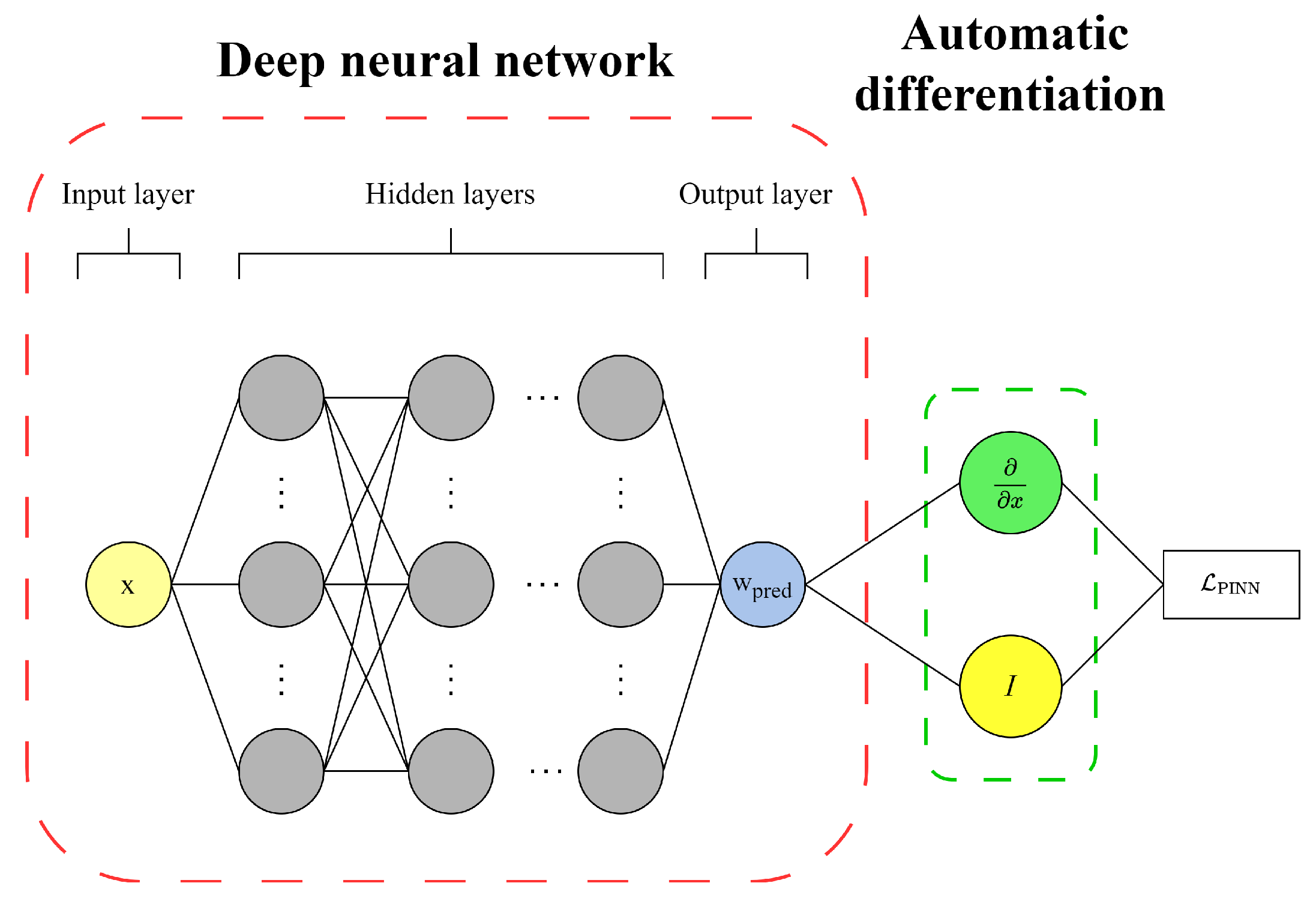
To achieve precise predictions of the beam’s displacement across an extensive parameter plane, a PINN-based surrogate model is constructed, as depicted in Figure 8. The outputs from the 15 PINN models presented in the previous section serve as the comprehensive training dataset for this surrogate model. The methodology and essential steps are outlined as follows:

The input data comprise 50 evenly spaced coordinate points selected within the range $y\in [-5\mathrm{m},5\mathrm{m}]$, along with the corresponding beam displacement predictions generated by the 15 pre-established target-domain PINN models. These inputs are denoted as $y_j$ (coordinate values) and $w_t^i\left(y_j\right)$ (displacement predictions), where $i=1,\dots ,15$ and $j=1,\dots ,50$. The output layer of the surrogate model represents the beam displacement predictions, matching the dimensionality of the input displacement values and denoted as $w_p^i\left(y_j\right)$, with $i=1,\dots ,15$ and $j=1,\dots ,50$. To construct the feedforward neural network architecture, a structured weight constraint approach is employed to define the mapping relationship between the output layer $w_p^i\left(y_j\right)$ and the input layers $y_j$ and $w_t^i\left(y_j\right)$. 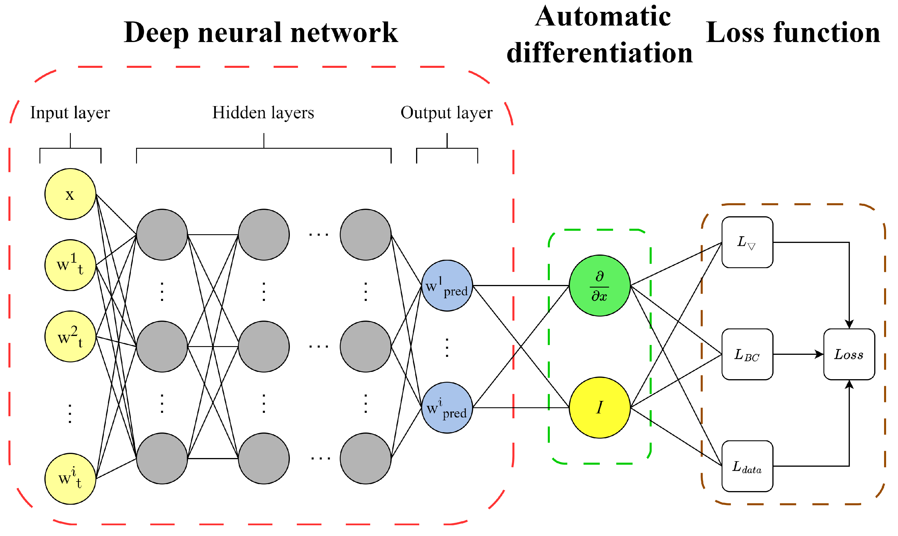Sparsity constraints are imposed on the network’s weight matrix M and bias vector b to enforce selective connectivity during training. This ensures that each neuron’s output is influenced exclusively by its corresponding input channel, while non-essential connections are pruned by constraining their weights to zero. This optimization strategy can be formally represented as

$$w_{\mathrm{p}}^i\left(y_j\right)=tanh·(M_{ii}·\left[y_j,w_{\mathrm{t}}^i\left(y_j\right)\right]+b_i),i=1,\dots ,15;j=1,\dots ,50,$$

(32)

where tanh is the activation function, and $M_{ii}$ denotes the diagonal elements of the weight matrix.

The loss function for the PINN surrogate model is formulated as an ensemble of loss functions derived from multiple local PINN models. This formulation is expressed as

$$\begin{array}{cc}\hfill L_{data}& ={\displaystyle \frac{1}{50}}·\sum _{i=1}^{15}\sum _{j=1}^{50}{\left|w_{\mathrm{p}}^i\left(y_j\right)-w_{\mathrm{t}}^i\left(y_j\right)\right|}^2\hfill \\ \hfill L_{▿}& ={\displaystyle \frac{1}{50}}·\sum _{i=1}^{15}\sum _{j=1}^{50}{\left|f^i\left(y_j\right)\right|}^2\hfill \end{array}$$

(33)

The PINN surrogate model differs from local PINN models in that it must handle a significantly larger dataset, leading to considerably higher computational costs during training. To address this, the surrogate model constructed in this study adopts a three-layer fully connected architecture (20 neurons per layer) with the “tanh” activation function. For data partitioning, a 4:1 ratio is implemented to divide the training set and validation set. The model training employs an adaptive learning rate scheduling strategy, where the initial learning rate is set to $1\times {10}^{-3}$ and halved every 200 training epochs. A dual early-stopping mechanism is triggered when the learning rate decays below the $1\times {10}^{-6}$ threshold or when the validation loss shows no downward trend for 30 consecutive epochs. Additionally, the surrogate model’s training employs the Adam optimizer. Training iterations are increased to 20,000. Notably, to prevent interference from sparsity constraints (e.g., L1/L2 regularization) with the physical governing equation loss terms, these regularization components have been intentionally excluded from the model design. In terms of prediction mechanism design, the surrogate model adopts a dynamic network activation strategy based on the domain features of the parameter space. More specifically, for a given prediction point $(c^{*},v^{*})$, the closest target-domain reference model within the parameter plane is first identified using the minimum Euclidean distance criterion, as follows:

$$d_i=\sqrt{{(c^{*}-c_i)}^2+{(v^{*}-v_i)}^2},i\in [1,15].$$

(34)

The surrogate model activates the sub-network module corresponding to the nearest neighbor model. The target parameter coordinates $(c^{*},v^{*})$ and the beam coordinate $y^{*}$ are then fed into this sub-network module simultaneously for deflection prediction. This mechanism significantly enhances the model’s ability to represent local features by preserving the domain-specific characteristics inherent to the parameter space.

To assess the model’s generalization capability, this study creates a 15 × 10 grid of test points in the parameter space, defined by $c\in [0.5,1,1.5,\dots ,5]\times {10}^6$ and $v\in [10,15,20,\dots$$,80]$, totaling 150 test points. For each test point, 400 equidistant points are positioned within a 5 m span both ahead of and behind the moving load on the beam to predict deflection. We use the metrics MAE (mean absolute error), RMSE (root mean square error), and coefficient of determination $R^2$ to evaluate the accuracy of model predictions. The formulations for MAE and RMSE are expressed as

$$MAE={\displaystyle \frac{1}{n}}\sum _{i=1}^n|w_{\mathrm{p}}^i\left(y_j\right)-w_{\mathrm{t}}^i\left(y_j\right)|$$

(35)

$$RMSE=\sqrt{{\displaystyle \frac{1}{n}}{\sum }_{i=1}^n{(w_{\mathrm{p}}^i\left(y_j\right)-w_{\mathrm{t}}^i\left(y_j\right))}^2}$$

(36)

where n is the number of sample data points, and $w_p^i\left(y_j\right)$ and $w_t^i\left(y_j\right)$ represent the predicted and actual displacement values, respectively.

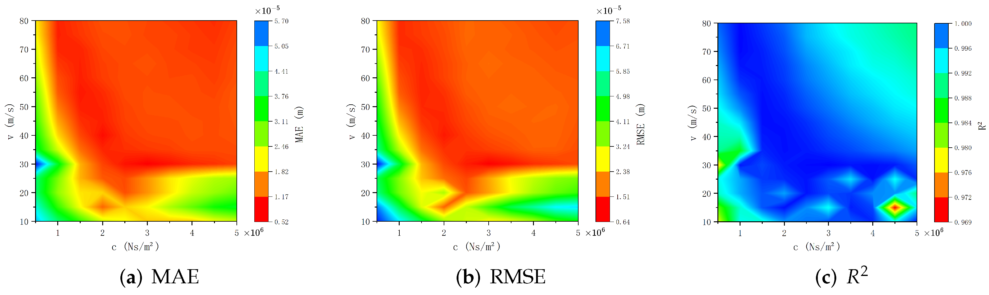
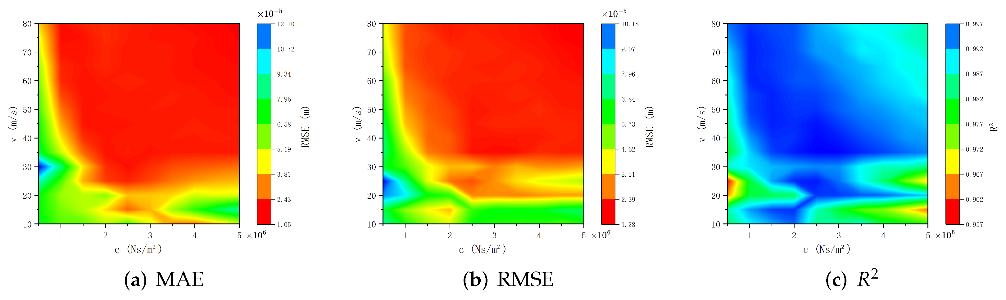
The evaluation values for each parameter point are mapped onto the $c-v$ parameter plane, resulting in the contour plot shown in Figure 9. Figure 9 demonstrates the prediction accuracy of the surrogate models through three evaluation metrics (MAE, RMSE, and $R^2$). Numerical experiments reveal that, in most parameter regions, the MAE and RMSE values are approximately ${10}^{-6}$, with $R^2$ values approaching 1. Next, we incrementally increase the noise intensity by introducing controlled noise levels equivalent to 2% and 3% of the maximum amplitude of the analytical solutions. 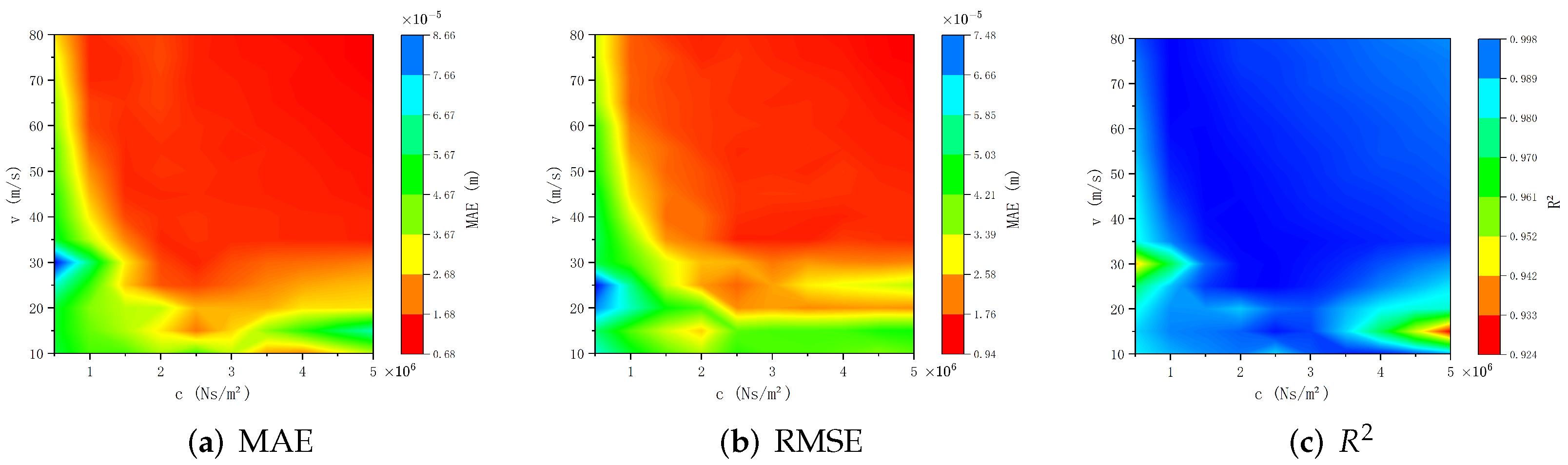Figure 10 and Figure 11 visually present the prediction results of the PINN surrogate model under higher noise standard deviation through MAE, RMSE, and $R^2$. The figures show that as the noise standard deviation increase, MAE and RMSE values for extreme outliers rise; however, in most parameter regions of the model, MAE and RMSE only slightly increase to approximately ${10}^{-5}$, with $R^2$ remaining close to 1. This indicates that the surrogate model possesses good robustness against noise.

6. Comparison of Result Accuracy with Existing PINN-Based Surrogate Model

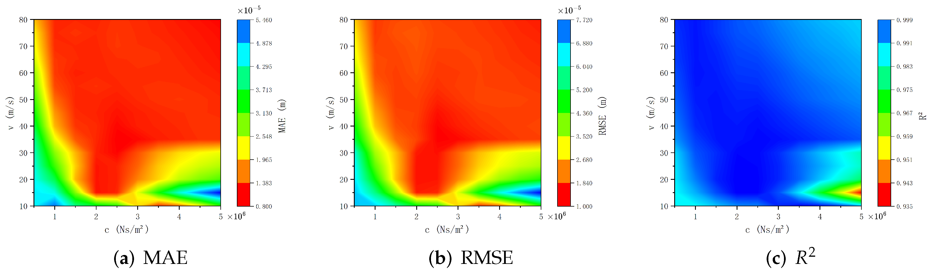
In contrast with existing PINN-based surrogate modeling techniques, our novel approach achieves a substantial reduction in data sampling requirements. Within a single source domain of the parameter space, merely 50 data points are sampled, spread over a 5 m span both ahead of and behind the moving load. Through the application of local PINN models, these 50 data points are augmented to 400. In Figure 12, Figure 13 and Figure 14, we present the prediction accuracy demonstration of the surrogate model trained with the existing method based on more data [21,22,23,32].

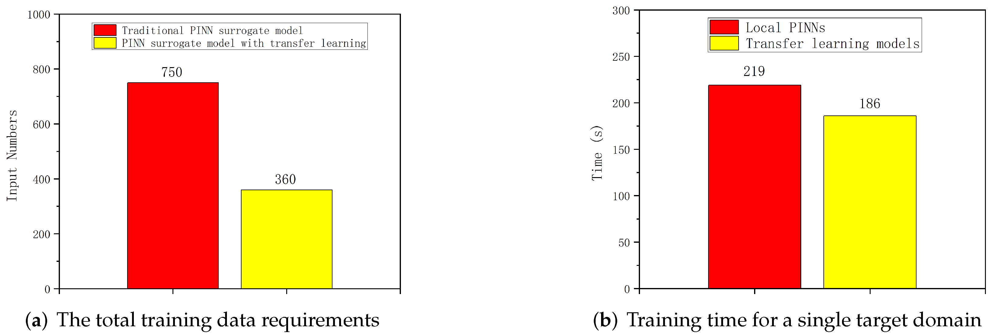
Compare Figure 12, Figure 13 and Figure 14 with Figure 9, Figure 10 and Figure 11. Although this augmentation process in our new approach may introduce a certain degree of inaccuracy when contrasted with measured values, it nonetheless maintains a satisfactory level of precision. Figure 15 illustrates a comparison of total data requirements and training time for a single target domain in the parameter space between our proposed method and the existing approach. The computer configuration utilized in our experiments is as follows: CPU AMD Ryzen 7 8845H with 8 cores, GPU NVIDIA GeForce RTX 4060 laptop, physical memory RAM 24 GB, and no GPU usage.

In the transfer learning phase, when transferring the local PINN model from the source domain to the target domain, a portion of the network layers of the local PINN model are frozen. Consequently, the target domain marks a substantial reduction from the source domain. Overall, in comparison with existing methods, our approach diminishes measured data sampling by a minimum of 50%. Furthermore, when transferring the local PINN model from the source to the target domain, only a minor fine-tuning of weights is necessary to attain commendable accuracy. In our numerical experiments, the training efficiency improves by 15% in comparison with conventional methods for a single target domain in the parameter space. The extent of efficiency enhancement is contingent upon the number of target domains, which subsequently determines the final accuracy of the surrogate model. By moderately relaxing the local precision requirements, our method attains significant improvements in computational efficiency and a marked reduction in data demand. This strategic trade-off allows for a more efficient computational process while still maintaining a satisfactory level of accuracy.

7. Discussion

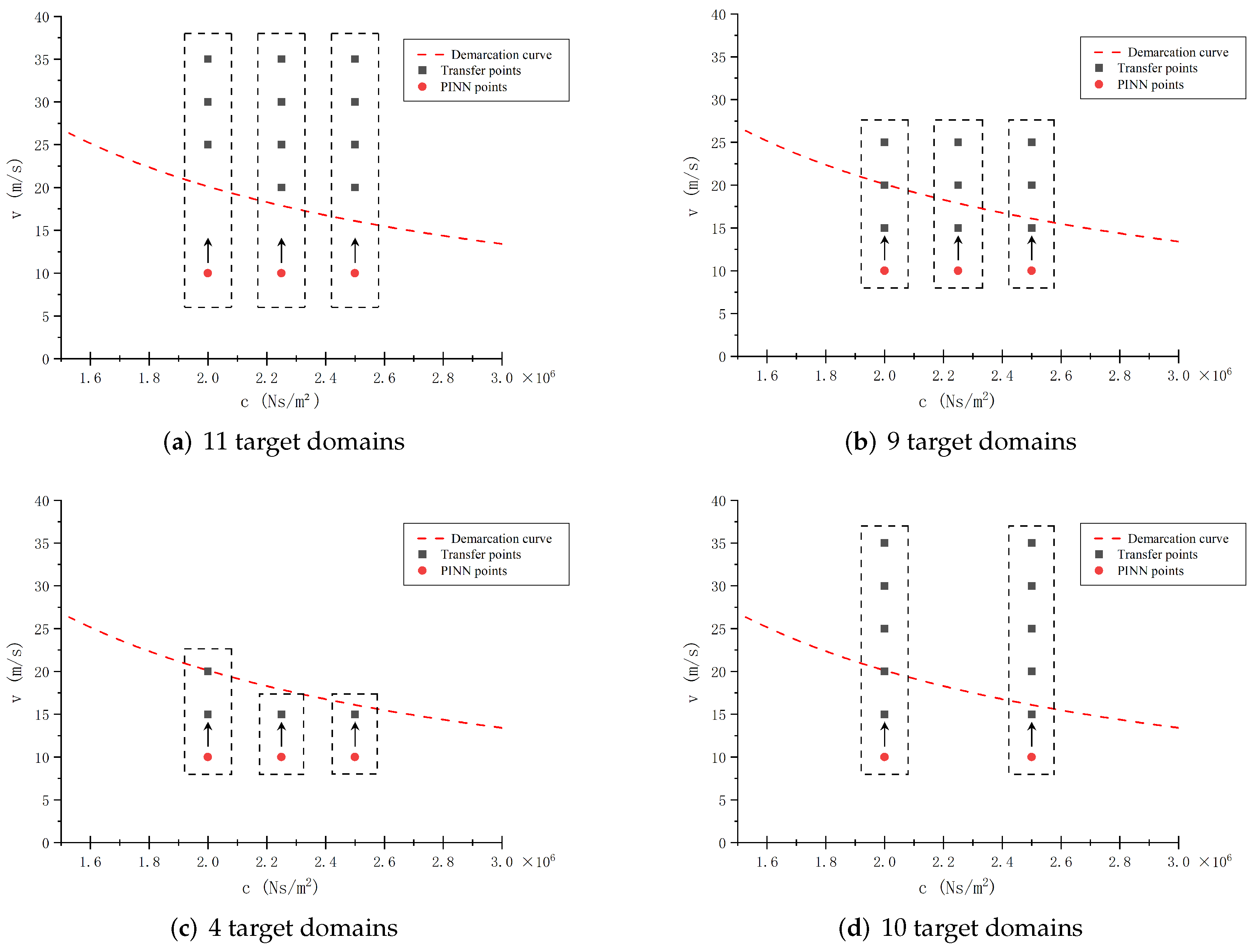
In this section, we conduct a systematic analysis of how migration path configurations impact the predictive accuracy of proposed PINN-based surrogate models. By examining the interactive effects of varying migration paths and noise levels on model performance, this evaluation provides critical insights into the reliability and robustness of the proposed surrogate models across diverse operational scenarios. Our findings deepen the understanding of how these factors collectively influence predictive capabilities and establish a foundation for optimizing transfer learning strategies in practical applications. We consider the following four distinct migration paths depicted in Figure 16:

• Figure 16a: Derived from the configuration in Figure 7, this path reduces the number of target domains from 15 to 11, with all target domains positioned above the demarcation curve in the parameter plane.
• Figure 16b: Building on Figure 7, the number of target domains is reduced from 15 to 9, and the target domains are distributed across both sides of the demarcation curve.
• Figure 16c: Extending from Figure 16b, the number of target domains is further reduced from 9 to 4, with both the source and target domains positioned below the demarcation curve.
• Figure 16d: Derived from Figure 7, this path reduces the number of source domains from 3 to 2 while decreasing the number of target domains from 15 to 10.

These configurations collectively allow for a thorough assessment of how transfer learning strategies perform across different levels of data sparsity and domain positioning. This evaluation provides critical insights into enhancing model reliability and robustness in practical applications.

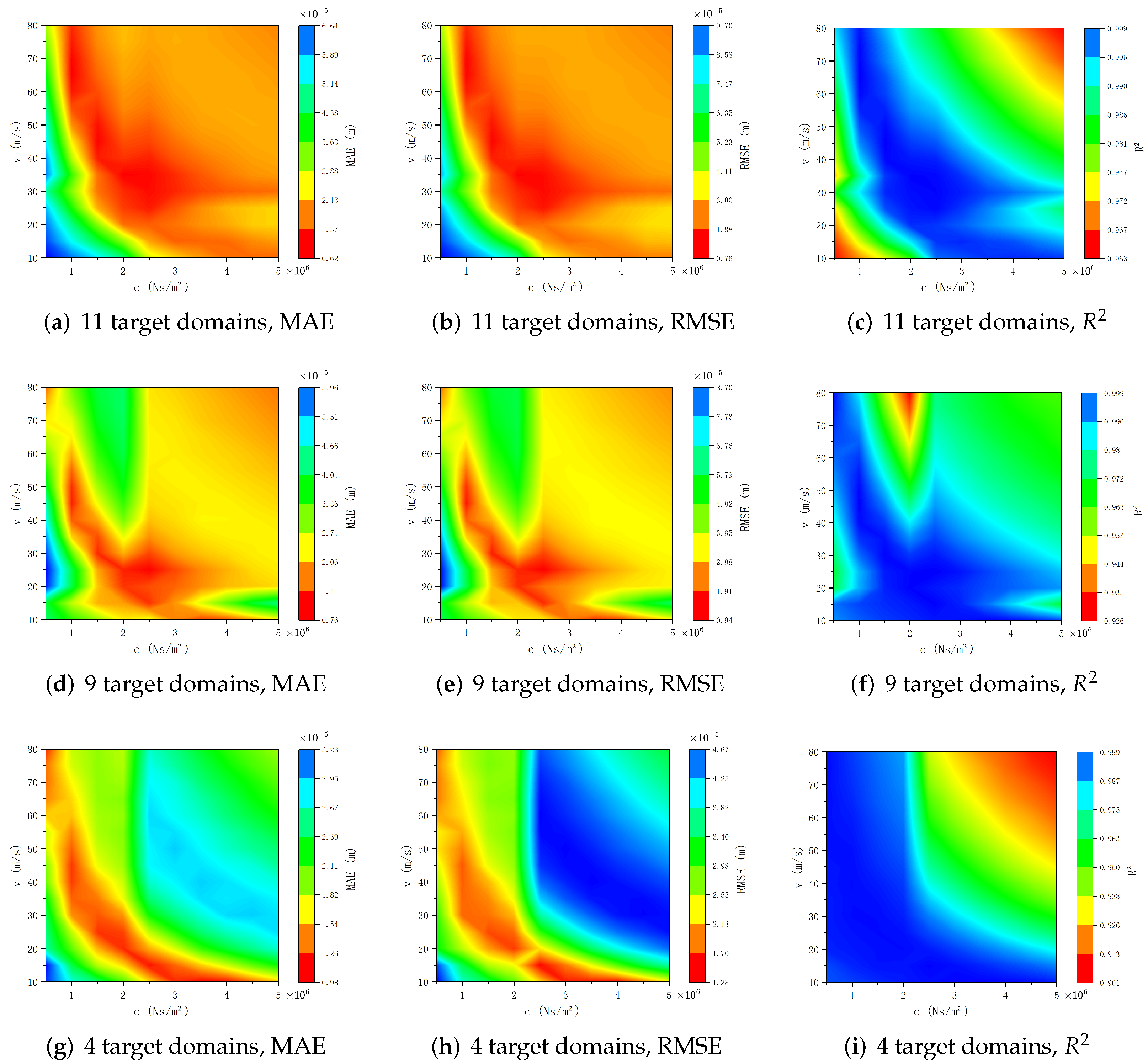
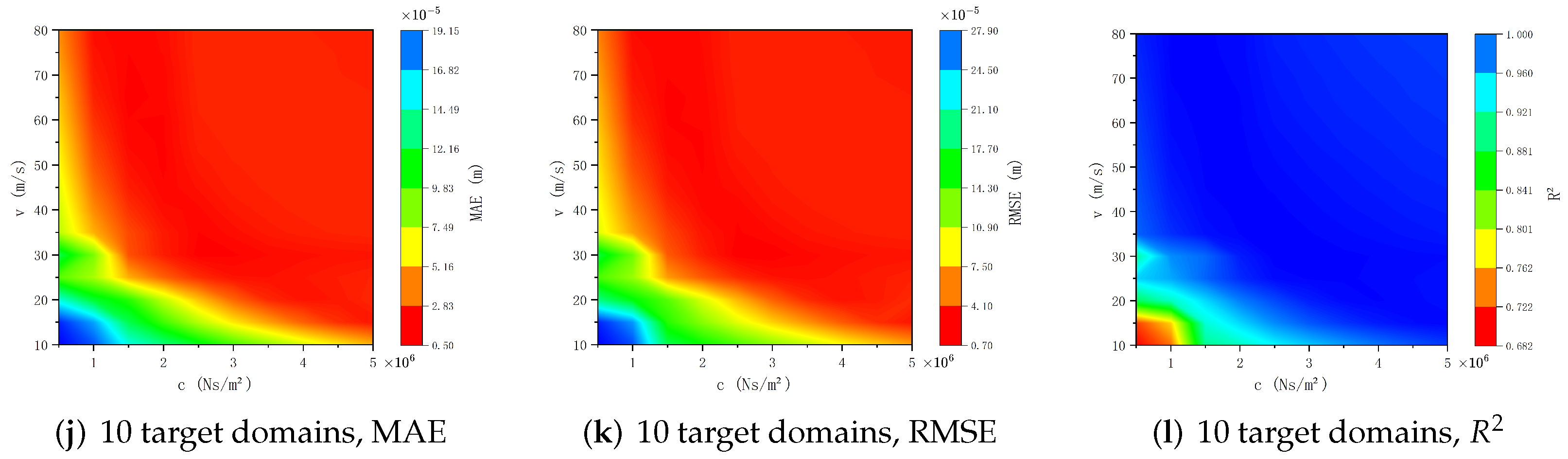
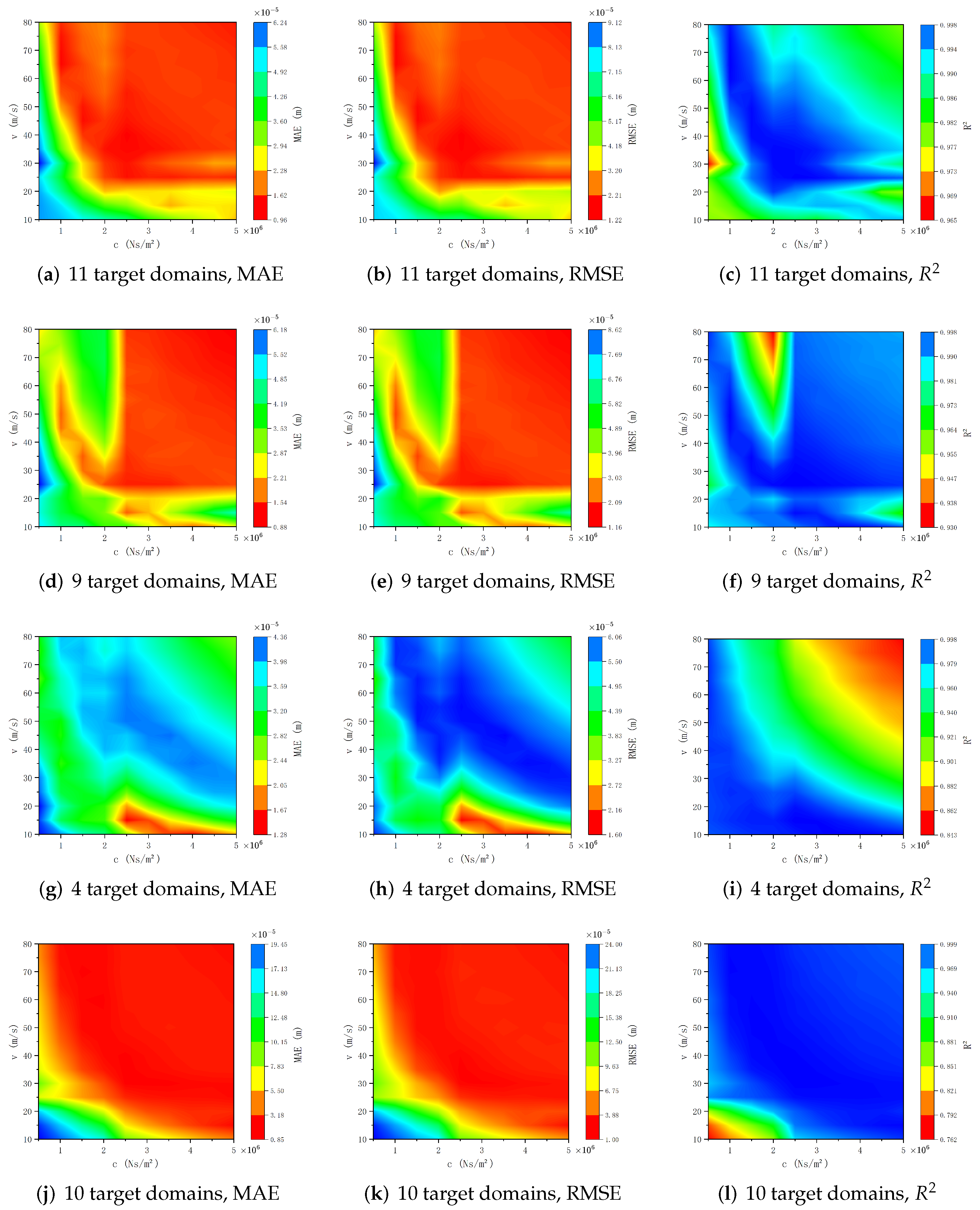
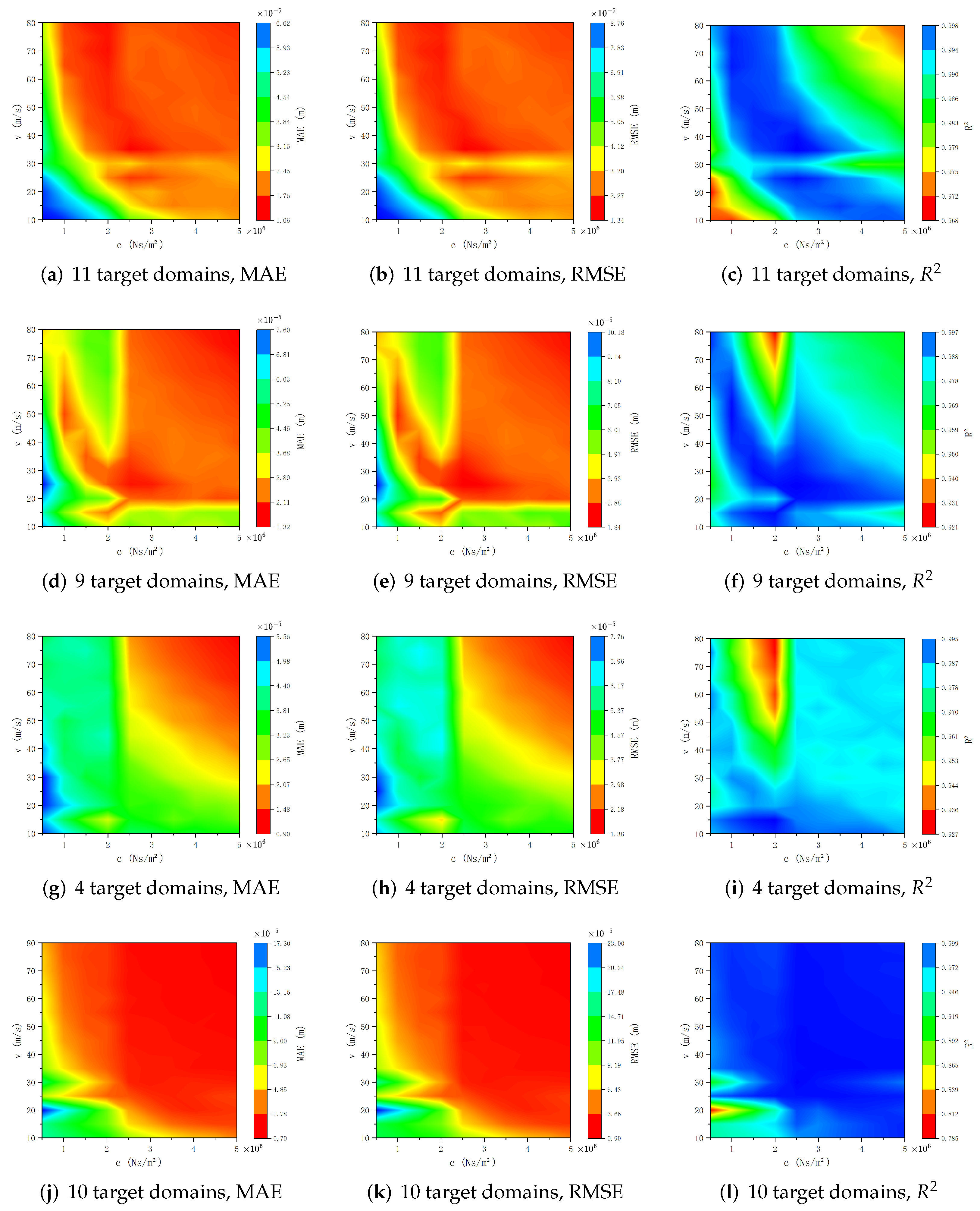
Figure 17, Figure 18 and Figure 19 depict how the four distinct migration paths illustrated in Figure 16 affect the surrogate model’s prediction accuracy under varying noise intensities, with noise standard deviations set at 1%, 2%, and 3% of the true value’s amplitude. Figure 17, Figure 18 and Figure 19 show that the transfer learning strategy on the $c-v$ parameter plane significantly impacts the surrogate model’s prediction accuracy. Under the same noise conditions, reducing the number of target domains leads to a corresponding drop in prediction accuracy. Moreover, when the number of target domains is progressively reduced while their distribution density in the occupied space remains largely unchanged, the surrogate model’s prediction accuracy consistently declines across the entire parameter plane. Conversely, when the distribution density of target domains in the occupied space is significantly reduced, the decline in prediction accuracy becomes notably non-uniform across the parameter plane, with some regions experiencing greater accuracy reductions than others (Figure 17j–l, Figure 18j–l, and Figure 19j–l). This spatially heterogeneous accuracy reduction underscores the importance of both the number and spatial organization of target domains in determining the surrogate model’s performance. To enhance the surrogate model’s reliability and robustness, particularly in complex modeling scenarios where data sparsity may be a concern, it is crucial to maintain adequate distribution density of target domains and strategically optimize their spatial arrangement.

Analysis of Figure 17, Figure 18 and Figure 19 shows that noise intensity significantly affects the surrogate model’s prediction accuracy, with a clear decline as the noise standard deviation increases. Notably, even when the noise standard deviation reaches 3% of the true amplitude and the number of target domains is reduced to just four, the surrogate model developed in this study maintains high prediction accuracy. The prediction MAE and RMSE are both maintained at ${10}^{-5}$ across the whole parameter space, while $R^2$ achieves values of 0.927 or higher across the parameter plane (Figure 19g–i). These results emphasize the model’s robustness and reliability, demonstrating its ability to provide accurate predictions even with significant noise and limited target domain data. This performance demonstrates the model’s practical applicability in real-world scenarios where data quality and quantity may be limited.

In Section 2, our theoretical analysis identifies a demarcation curve on the $c-v$ parameter plane, where the beam’s vibration responses vary in form across this boundary. When all target domains lie below this curve (Figure 16c), the surrogate model’s prediction accuracy exhibits marked differences above and below the boundary, particularly at low noise levels. This suggests that classifying the solutions to the governing equations can inform the selection of optimal migration paths, thereby boosting the surrogate model’s overall prediction accuracy.

8. Conclusions

This study presents a novel PINN-based surrogate modeling framework for predicting the steady-state dynamic response of infinite E–B beams on foundations under moving loads across broad parameter ranges. Our methodology involves (1) constructing localized PINN models trained on displacement data from specific points in the damping-velocity parameter space and (2) employing transfer learning techniques to generalize these models across different parameter regions. The key innovation of our approach lies in its ability to maintain high prediction accuracy while substantially reducing data requirements compared with conventional PINN-based surrogate modeling methods. Numerical experiments demonstrate that when selecting 15 target domains, our method achieves comparable accuracy to traditional PINN surrogate models while requiring less than half the training data. For applications where minor accuracy reduction is acceptable, the number of target domains can be further reduced to 4.

Empirical results confirm the proposed surrogate model’s reliability and robustness under various noise conditions and transfer learning pathways. Notably, we find that simply increasing the number of target domains does not necessarily improve prediction accuracy. Instead, enhancing the spatial distribution density of target domains proves more effective for maintaining performance. These findings enable large-scale parameter prediction in data-limited scenarios while preserving computational efficiency. The proposed framework represents a significant advancement in data-efficient surrogate modeling, demonstrating particular effectiveness in high-accuracy prediction with minimal training data, robust performance across diverse parameter conditions, and adaptability to noisy measurement environments. This work establishes a foundation for efficient dynamic response prediction in scenarios where experimental data collection is challenging or costly.

Existing PINN-based surrogate models often suffer from low training efficiency, primarily due to their dependence on extensive datasets. To address this limitation, we propose a novel method for predicting the steady-state response of infinite beams on foundations subjected to moving loads, particularly in scenarios where only sparse measurement data are available under constrained parameter conditions. A key practical challenge in our approach lies in balancing the trade-off between data requirements and predictive accuracy in surrogate modeling. Our numerical experiments demonstrate that partitioning the solution manifold into well-defined parameter regions enables the identification of optimal transfer learning pathways, thereby significantly improving model performance, especially in data-scarce regimes. Advancing this framework to optimize data efficiency and generalization capabilities will be the focus of our future research.

References

1. Fryba, L. Vibration of Solids and Structures Under Moving Loads, 3rd ed.; Thomas Telford Ltd.: London, UK, 1999. [Google Scholar]
2. Ouyang, H.J. Moving-load dynamic problems: A tutorial (with a brief overview). Mech. Syst. Signal Process. 2011, 25, 2039–2060. [Google Scholar] [CrossRef]
3. Koziol, P.; Hryniewicz, Z. Dynamic response of a beam resting on a nonlinear foundation to a moving load: Coiflet-based solution. Shock Vib. 2012, 19, 995–1007. [Google Scholar] [CrossRef]
4. Miao, Y.; Shi, Y.; Luo, H.B.; Gao, R.X. Closed-form solution considering the tangential effect under harmonic line load for an infinite Euler–Bernoulli beam on elastic foundation. Appl. Math. Model. 2018, 54, 21–33. [Google Scholar] [CrossRef]
5. Rodrigues, C.; Simoes, F.M.F.; Costa, A.P.D.; Froio, D.; Rizzi, E. Finite element dynamic analysis of beams on nonlinear elastic foundations under a moving oscillator. Eur. J. Mech. Solids 2018, 68, 9–24. [Google Scholar] [CrossRef]
6. Bi, S.; Beer, M.; Mottershead, J. Recent advances in stochastic model updating. Mech. Syst. Signal Process. 2022, 172, 108971. [Google Scholar] [CrossRef]
7. Moon, H.S.; Ok, S.; Chun, P.; Lim, Y.M. Artificial neural network for vertical displacement prediction of a bridge from strains (Part 1): Girder bridge under moving vehicles. Appl. Sci. 2019, 9, 2881. [Google Scholar] [CrossRef]
8. Nguyen, T.Q. A data-driven approach to structural health monitoring of bridge structures based on the discrete model and FFT-deep learning. J. Vib. Eng. Technol. 2021, 9, 1959–1981. [Google Scholar] [CrossRef]
9. Marasco, G.; Piana, G.; Chiaia, B.; Ventura, G. Genetic algorithm supported by influence lines and a neural network for bridge health monitoring. J. Struct. Eng. 2022, 148, 04022123. [Google Scholar] [CrossRef]
10. Ye, X.; Jin, T.; Yun, C. A review on deep learning-based structural health monitoring of civil infrastructures. Smart Struct. Syst. 2019, 24, 567–585. [Google Scholar]
11. Karniadakis, G.E.; Kevrekidis, I.G.; Lu, L.; Perdikaris, P.; Wang, S.F.; Yang, L. Physics-informed machine learning. Nat. Rev. Phys. 2021, 3, 422–440. [Google Scholar] [CrossRef]
12. Avci, O.; Abdeljaber, O.; Kiranyaz, S.; Hussein, M.; Gabbouj, M.; Inman, D.J. A review of vibration-based damage detection in civil structures: From traditional methods to Machine Learning and Deep Learning applications. Mech. Syst. Signal Process. 2021, 147, 107077. [Google Scholar] [CrossRef]
13. Raissi, M.; Perdikaris, P.; Karniadakis, G.E. Physics-informed neural networks: A deep learning framework for solving forward and inverse problems involving nonlinear partial differential equations. J. Comput. Phys. 2019, 378, 686–707. [Google Scholar] [CrossRef]
14. Blechschmidt, J.; Ernst, O.G. Three ways to solve partial differential equations with neural networks—A review. Gamm-Mitteilungen 2021, 44, e202100006. [Google Scholar] [CrossRef]
15. Cuomo, S.; Di-Cola, V.S.; Giampaolo, F.; Rozza, G.; Raissi, M.; Piccialli, F. Scientific machine learning through physics–informed neural networks: Where we are and what’s next. J. Sci. Comput. 2022, 92, 88. [Google Scholar] [CrossRef]
16. Kapoor, T.; Wang, H.; Nunez, A.; Dollevoet, R. Physics-informed neural networks for solving forward and inverse problems in complex beam systems. In IEEE Transactions on Neural Networks and Learning Systems; IEEE: New York, NY, USA, 2023. [Google Scholar]
17. Kapoor, T.; Wang, H.; Nunez, A.; Dollevoet, R. Physics-informed machine learning for moving load problems. J. Phys. Conf. Ser. 2024, 2647, 152003. [Google Scholar] [CrossRef]
18. Fallah, A.; Aghdam, M.M. Physics-informed neural network for bending and free vibration analysis of three-dimensional functionally graded porous beam resting on elastic foundation. Eng. Comput. 2023, 40, 437–454. [Google Scholar] [CrossRef]
19. Li, Y.F.; He, W.Y.; Ren, W.X.; Shao, Y.H. Moving load induced dynamic response analysis of bridge based on physics-informed neural network. Adv. Eng. Inform. 2025, 65, 103215. [Google Scholar] [CrossRef]
20. Chen, Z.L.; Lai, S.K.; Yang, Z.C. At-pinn: Advanced time-marching physics-informed neural network for structural vibration analysis. Thin-Walled Struct. 2024, 196, 111423. [Google Scholar] [CrossRef]
21. Zhang, W.; Su, Y.; Jiang, Y.; Hu, Z.; Bi, J.; He, W. Data-driven fatigue crack propagation and life prediction of tubular T-joint: A fracture mechanics based machine learning surrogate model. Eng. Fract. Mech. 2024, 311, 110556. [Google Scholar] [CrossRef]
22. Ng, C.W.W.; Zhou, Q.; Zhang, Q. A novel surrogate model for hydro-mechanical coupling in unsaturated soil with incomplete physical constraints. Comput. Geotech. 2025, 180, 107091. [Google Scholar] [CrossRef]
23. Liu, K.; Luo, K.; Cheng, Y.; Liu, A.; Li, H.; Fan, J.; Balachandar, S. Surrogate modeling of parameterized multi-dimensional premixed combustion with physics-informed neural networks for rapid exploration of design space. Combust. Flame 2023, 258, 113094. [Google Scholar] [CrossRef]
24. Pan, S.J.; Yang, Q. A survey on transfer learning. IEEE Trans. Knowl. Data Eng. 2010, 22, 1345–1359. [Google Scholar] [CrossRef]
25. Tan, C.; Sun, F.; Kong, T.; Zhang, W.C.; Yang, C.; Liu, C.F. A survey on deep transfer learning. In Proceedings of the International Conference on Artificial Neural Networks, Rhodes, Greece, 4–7 October 2018. [Google Scholar]
26. Niu, S.T.; Liu, Y.X.; Wang, J.; Song, H.B. A decade survey of transfer learning (2010–2020). IEEE Trans. Artif. Intell. 2020, 1, 151–166. [Google Scholar] [CrossRef]
27. Zhao, Z.H.; Alzubaidi, L.; Zhang, J.L.; Duan, Y.; Gu, Y.T. A comparison review of transfer learning and self-supervised learning: Definitions, applications, advantages and limitations. Expert Syst. Appl. 2024, 242, 122807. [Google Scholar] [CrossRef]
28. Li, M.Y.; Li, Y.; Li, Z.M. A comprehensive survey of transfer dictionary learning, Neurocomputing. Neurocomputing 2025, 623, 129322. [Google Scholar] [CrossRef]
29. Zhang, N.; Xu, K.P.; Yin, Z.Y.; Li, K.Q. Transfer learning-enhanced finite element-integrated neural networks. Int. J. Mech. Sci. 2025, 290, 110075. [Google Scholar] [CrossRef]
30. Zhao, T.; Wang, X.; Song, X. Multiobjective backbone network architecture search based on transfer learning in steel defect detection. Neurocomputing 2025, 635, 130012. [Google Scholar] [CrossRef]
31. Wu, T.; Thompson, D.J. The effects of track non-linearity on wheel/rail impact. Proc. Inst. Mech. Eng. Part F J. Rail Rapid Transit. 2004, 218, 1–15. [Google Scholar] [CrossRef]
32. Go, M.-S.; Noh, H.-K.; Lim, J.H. Real-time full-field inference of displacement and stress from sparse local measurements using physics-informed neural networks. Mech. Syst. Signal Process. 2025, 224, 112009. [Google Scholar] [CrossRef]
Figure 1. The diagrammatic representation of an infinite E–B beam on a foundation subjected to a moving load.
Applsci 15 06213 g001
Figure 2. Comparisons between analytical and numerical results for w under the parameters given in Equation (25) are as follows: (a) the curves of g μ 0 ( c , v ) = 0 in the c v parameter plane (defined in Equation (19)), with g μ 0 ( c , v ) < 0 in the shaded region; (b) w for point ψ 1 ; (c) w for point ψ 2 ; and (d) w for point ψ 3 .
Applsci 15 06213 g002
Figure 3. Schematic diagram of local PINN framework.
Applsci 15 06213 g003
Figure 4. The training convergence curves for all six network topologies ( S 1 S 6 ) defined in Table 1.
Applsci 15 06213 g004
Figure 5. Comparison between the prediction results of the PINN models and the results obtained from the analytical solutions (27) and (28) for three points ( c , v ) = { ( 2.0 × 10 6 , 10 ) , ( 2.25 × 10 6 , 10 ) , ( 2.5 × 10 6 , 10 ) } . The remaining parameters are derived from Equation (25) in Section 2, while the magnitude of the moving load is adjusted to P = 10 3 ( k N ) . (a) Comparison of true and predicted values for point ( c , v ) = ( 2.0 × 10 6 , 10 ) . (b) Prediction error for point ( c , v ) = ( 2.0 × 10 6 , 10 ) . (c) Comparison of true and predicted values for point ( c , v ) = ( 2.25 × 10 6 , 10 ) . (d) Prediction error for point ( c , v ) = ( 2.25 × 10 6 , 10 ) . (e) Comparison of true and predicted values for point ( c , v ) = ( 2.5 × 10 6 , 10 ) . (f) Prediction error for point ( c , v ) = ( 2.5 × 10 6 , 10 ) .
Applsci 15 06213 g005
Figure 6. Process of a transfer learning strategy with layer-wise parameter freezing.
Applsci 15 06213 g006
Figure 7. The migration path on the c v parameter plane. Arrows represent the direction of migration paths.
Applsci 15 06213 g007
Figure 8. Schematic diagram of the PINN-based surrogate model.
Applsci 15 06213 g008
Figure 9. Contour plot of (a) MAE, (b) RMSE, and (c) R 2 values for our PINN surrogate model on the c v parameter plane. The noise standard deviation is set to 1% of the true values’ amplitude.
Applsci 15 06213 g009
Figure 10. Contour plot of (a) MAE, (b) RMSE, and (c) R 2 values for our PINN surrogate model on the c v parameter plane. The noise standard deviation is set to 2% of the true values’ amplitude.
Applsci 15 06213 g010
Figure 11. Contour plot of (a) MAE, (b) RMSE, and (c) R 2 values for our PINN surrogate model on the c v parameter plane. The noise standard deviation is set to 3% of the true values’ amplitude.
Applsci 15 06213 g011
Figure 12. Contour plot of (a) MAE, (b) RMSE, and (c) R 2 values for the existing PINN surrogate model on the c v parameter plane. The noise standard deviation is set to 1% of the true values’ amplitude.
Applsci 15 06213 g012
Figure 13. Contour plot of (a) MAE, (b) RMSE, and (c) R 2 values for the existing PINN surrogate model on the c v parameter plane. The noise standard deviation is set to 2% of the true values’ amplitude.
Applsci 15 06213 g013
Figure 14. Contour plot of (a) MAE, (b) RMSE, and (c) R 2 values for the existing PINN surrogate model on the c v parameter plane. The noise standard deviation is set to 3% of the true values’ amplitude.
Applsci 15 06213 g014
Figure 15. Comparison of (a) the total training data requirements and (b) training time for a single target domain in the parameter space between the proposed method and existing methods.
Applsci 15 06213 g015
Figure 16. Schematic diagram of four distinct migration paths on the c v parameter plane: (a) 11 target domains, (b) 9 target domains, (c) 4 target domains, and (d) 10 target domains. Arrows represent the direction of migration paths.
Applsci 15 06213 g016
Figure 17. The impact of different migration paths on the prediction accuracy of the proposed surrogate model illustrated through three evaluation metrics, MAE, RMSE, and R 2 . The noise standard deviation is 1% of the true value’s amplitude.
Applsci 15 06213 g017aApplsci 15 06213 g017b
Figure 18. The impact of different migration paths on the prediction accuracy of the proposed surrogate model illustrated through three evaluation metrics, MAE, RMSE, and R 2 . The noise standard deviation is 2% of the true value’s amplitude.
Applsci 15 06213 g018
Figure 19. The impact of different migration paths on the prediction accuracy of the proposed surrogate model illustrated through three evaluation metrics, MAE, RMSE, and R 2 . The noise standard deviation is 3% of the true value’s amplitude.
Applsci 15 06213 g019