Ensemble Method of Triple Naïve Bayes for Plastic Type Prediction in Sorting System Automation

Abstract

Recycling has been acknowledged as a viable alternative for the management of plastic refuse. An automatic sorting system is required by the industry to predict the plastic waste based on the type before it is recycled. The plastic sorting system automation requires intelligent computing as a software system that can predict the type of plastic accurately. The ensemble method is a method that combines several single prediction methods based on machine learning into an algorithm to obtain better performance. This study aims to build intelligent computing for the automation of digital image-based plastic waste sorting systems using an ensemble method built from three naïve Bayes single prediction methods. The three single models consist of one Naïve Bayes (NB) model with crisp discretization and two NB models with fuzzy discretization, namely those using a combination of linear–triangular fuzzy membership functions and a combination of linear–trapezoidal fuzzy membership functions. We hypothesize that the performance of each single model and the proposed ensemble model is different, and the performance of the ensemble model is higher than all the single models used to build it. The hypothesis is proven, and there is an increase in performance from each single method to the ensemble method ranging from 2.06% to 5.56%. The evidence of this hypothesis also shows that the performance of the proposed prediction model using the ensemble method built from three naive Bayes models is high and robust.

1. Introduction

The use of plastic is becoming more widespread in countries experiencing economic expansion [1]. Since 2000, plastic waste has more than doubled [2]. The 2023 Indonesian River Affairs Research Agency census conducted in 13 provinces shows that plastic waste is a major problem in Indonesia. The nature of plastic waste, which is difficult to decompose, has a very broad negative impact on various ecosystems, human health, and many species [3,4].

Recycling has been identified as a viable alternative for plastic waste management [5]. However, on the other hand, it can cause cross-contamination between types of plastic, thereby increasing industrial operational costs [6,7]. In the industrial process, plastic waste recycling requires an automatic sorting system to sort plastic waste based on its type. This system requires intelligent computing that should not only consider advanced technology in obtaining data, the number of samples, and the validation techniques used but also consider that the performance of the prediction model obtained is not only high but also robust, not because of luck or coincidence due to sampling carried out in the training and testing process. High, stable, and robust prediction performance will provide an effective and efficient sorting system [8,9].

In the current era of Industry 4.0, the use of digital images extracted into the chromatic model of Red, Green, and Blue (RGB) as datasets in solving prediction or identification-related problems is increasing rapidly because it is cheaper than other technologies [10], such as multi-wavelength transmission spectrum [7], image sensor [4], laser [11], or infrared sensor [12,13,14]. Some infrared sensor technologies that use spectroscopy are claimed to be low cost, but the prediction performance of the intelligent system that is built is still not satisfactory, with performance metrics below 73% [14], or the performance obtained uses very few samples [7,12], or the performance obtained is not yet robust because it is only based on one sampling [4,7,12,13,14].

Digital images processed using the chromatic model of RGB are generally more informative [15], have a real difference between the channel colors [16,17], and can also provide good predictive performance [18,19,20]. However, not all prediction methods in machine learning can directly process ratio-scale data generated by digital image processing to the chromatic model of RGB. In addition, the process of transforming ratio data to ordinal or nominal can produce ambiguous interval groups [21], especially digital image data processed into the RGB color space model [22,23], so the transformation carried out becomes inefficient [24]. Fuzzy discretization can overcome the problem of ambiguity in datasets [25,26], and in addition, it has the potential to enhance the prediction method’s efficacy [27,28]. Nevertheless, the prediction model’s efficacy with fuzzy discretization is significantly influenced by the combination of fuzzy membership functions employed [22,29].

The main challenge in building and developing intelligent computing is to obtain high, stable, and robust prediction performance. The ensemble method is a method that combines several single prediction methods based on machine learning into an algorithm to obtain better performance [30]. This method is one of the solutions when a single prediction method does not provide satisfactory prediction performance [31]. This method can also reduce prediction variance [32] and increase the robustness of the performance of a single method [33,34]. However, not all combinations of single prediction methods into ensemble methods provide good performance [31,34]. In-depth research is needed regarding the combination of single prediction methods that build it.

For this reason, this study aims to build and develop intelligent computing for the sorting system automation of plastic waste based on digital images using an ensemble method constructed from three basic prediction methods based on the Naïve Bayes (NB) model. The novelty of this work is the construction of an ensemble model based on three single NB models to predict three types of plastic as an intelligent system in sorting automation. One NB model with crisp discretization and two NB models with fuzzy discretization are the components of three basic models. For fuzzy discretization models, they are combinations of linear–trapezoidal fuzzy membership functions and linear–triangular fuzzy membership functions. Both combinations of fuzzy membership functions provide superior performance in several applications [22,29]. We hypothesize that the performance of the three NB-based basic models and the suggested ensemble models is different and that at least one of the suggested ensemble models has a higher performance than all NB-based single models.

2. Materials and Methods

2.1. Materials

The digital images of plastic waste that were deposited on a conveyor belt were captured to obtain the material for this work. The digital images were subsequently transformed into a chromatic model of the RGB and produced numerical data with a ratio scale. The capturing process is given in Figure 1.

This research involved three types of plastic that are commonly used in society and can decompose into waste as the dataset: Polyethylene Terephthalate (PET/PETE), High-Density Polyethylene (HDPE), and Polypropylene (PP). Samples of each type were 150 different objects, so the total sample was 450. Digital images of the objects were obtained through the capture process at random poses using a webcam with automatic lighting. We then processed the images using the RGB color model. This study’s plastic objects were intact and undamaged and had previously undergone a thorough cleaning to remove all dirt attachments.

2.2. Methods

Model development begins with transforming data from numerical form to categorical form using discretization, consisting of crisp discretization and fuzzy discretization. Each is built based on the notion of crisp and fuzzy set membership. In the notion of crisp set, an entry of universal $X$ is denoted as $x\in A$ if it is a member of set $A$. On the contrary, if $x$ is not an entry of $A$, it is denoted as $x\notin A$. Consequently, the membership degree of $x$ in set $A$ is limited to either 1 or 0, which is written as ${\mu }_A\left(x\right)=1$or ${\mu }_A\left(x\right)=0$ [22]. In the notion of fuzzy set, the membership degree $x$ in set $A$ is contained in the range [0, 1]. This value is formulated in a function called the fuzzy membership function. This function shows the value of the membership of each value in a given fuzzy set ${\tilde{X}}_d$. If $x$ possesses the highest membership value, it is considered a member of set $A$ [22,35].

The number of categories in each predictor variable is determined by antecedent information or expert justification in crisp discretization, and the interval boundaries between categories are distinct [22,29]. Determining the category interval limits for each numeric variable with a ratio scale using (1), ${x_d}^o$ and $x_d$are the $d$-th continuous and the $d$-th discretized predictor variable values, respectively [22]:

$$x_d={x_d}^o+\mathrm{R}\mathrm{a}\mathrm{n}\mathrm{g}\mathrm{e}\left({x_d}^o\right)$$

(1)

The number of categories in fuzzy discretization is determined by the categories that are established through crisp discretization, but it also accommodates overlapping class intervals [22]. Each variable is discretized through three categories, and each category is represented by a single fuzzy membership function. Suppose $X$is the universal set of the fuzzy set, ${\tilde{X}}_d,$ with element $x_f$ and membership function ${\mu }_{{\tilde{X}}_d}\left(x_f\right)$, then the fuzzy set ${\tilde{X}}_d$ is the ordered pairs of each $x_f$ and ${\mu }_{{\tilde{X}}_d}\left(x_f\right)$ [35]:

$${\tilde{X}}_d=\left\{\left(x_f,{\mu }_{{\tilde{X}}_d}\left(x_f\right)\right)|x_f\in X\right\}$$

(2)

The fuzzy membership function ${\mu }_{{\tilde{X}}_d}\left(x_f\right)$ is defined as ${\mu }_{{\tilde{X}}_d}\left(x_f\right):X \to \left[0, 1\right]$, and every element $x_f$ of $X$ is assigned a value within the interval [0, 1].

Naïve Bayes is a high-performance method for making predictions based on digital images [36,37], especially those that handle the vagueness that results from discretization [22]. However, sometimes this method also does not provide satisfactory performance [38]. The ensemble method is a machine learning-based algorithm that integrates multiple single prediction methods to enhance performance [30]. This technique is one of the solutions available when the prediction performance of a single prediction method is not satisfactory [31].

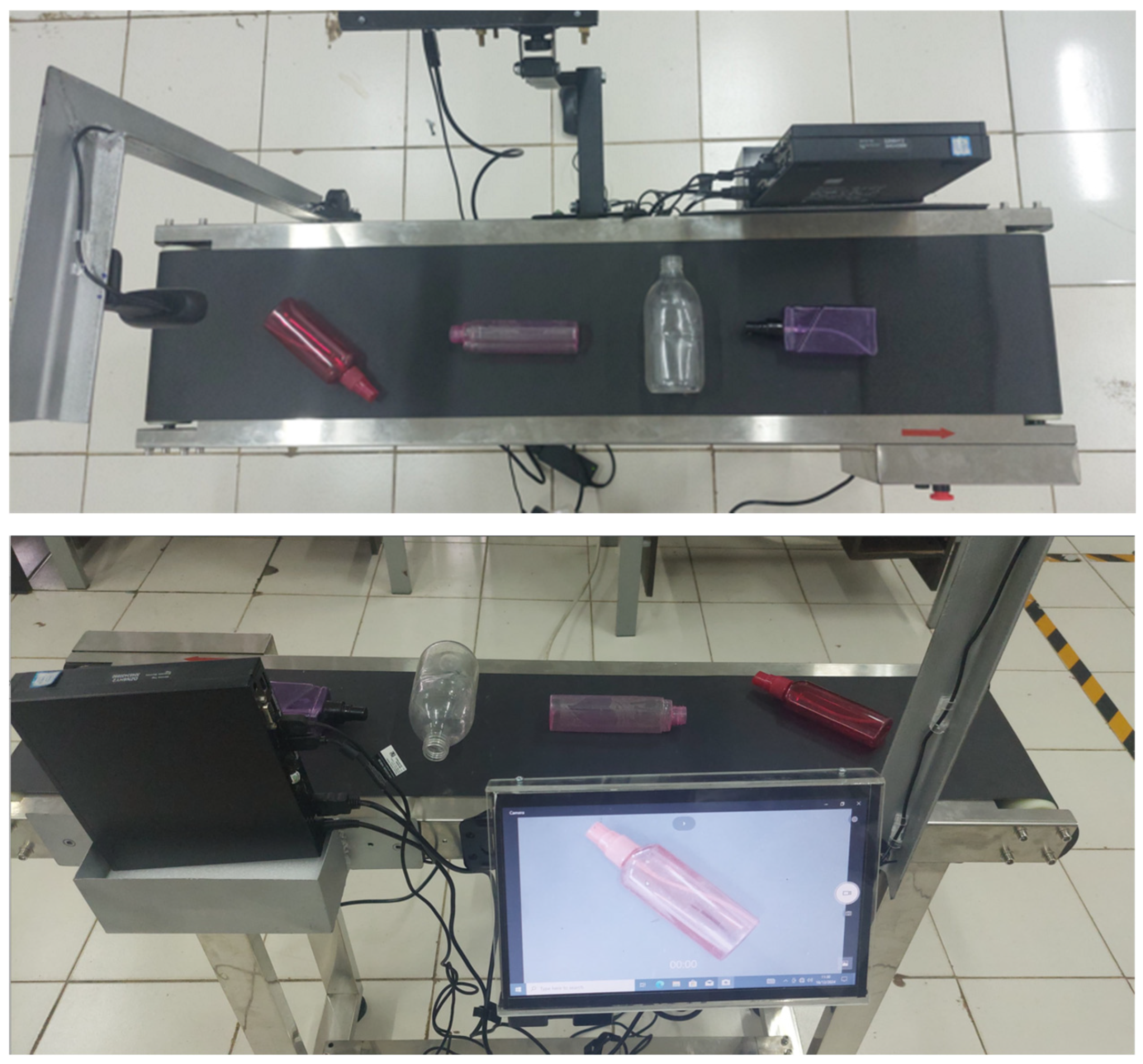
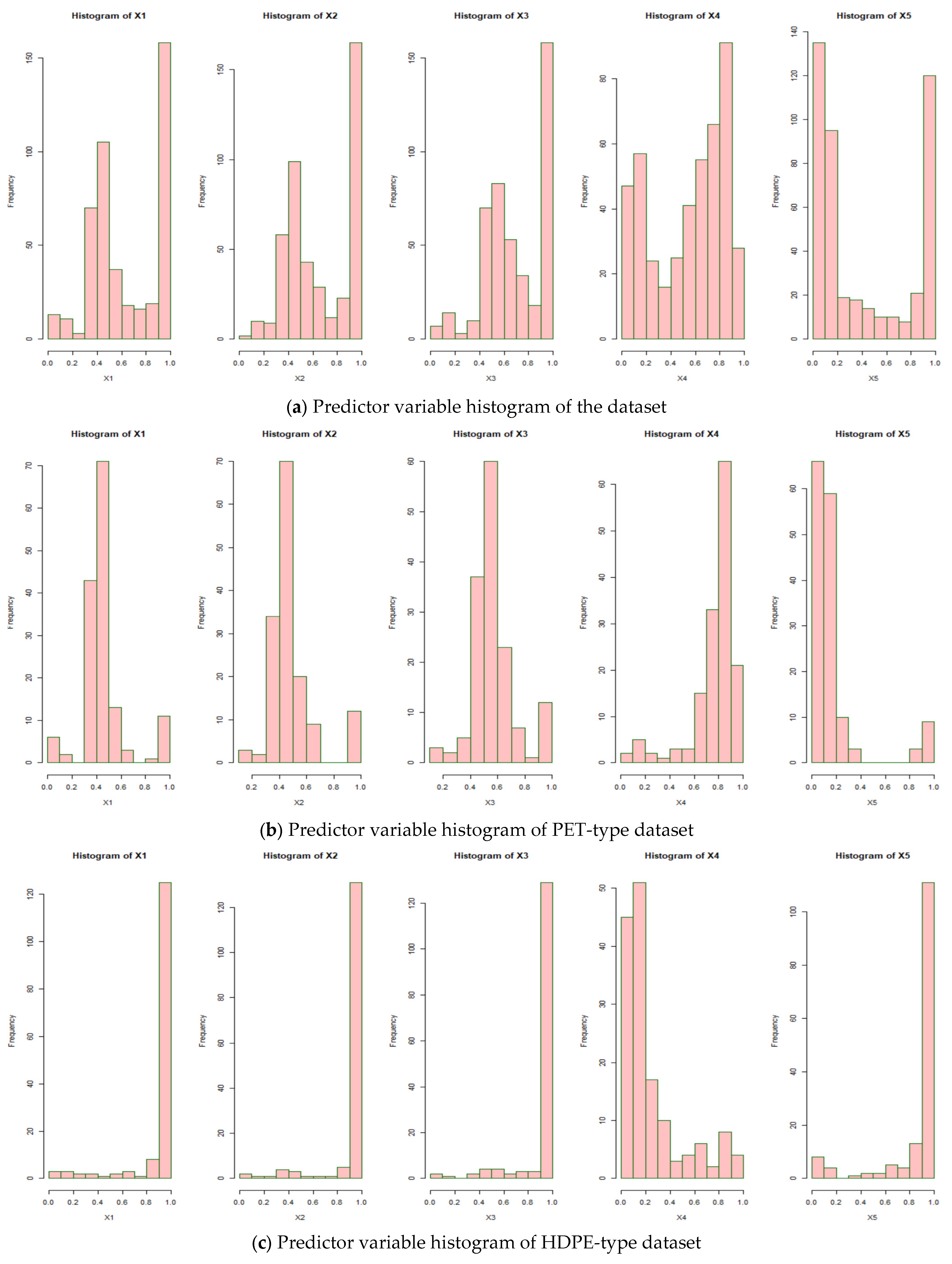
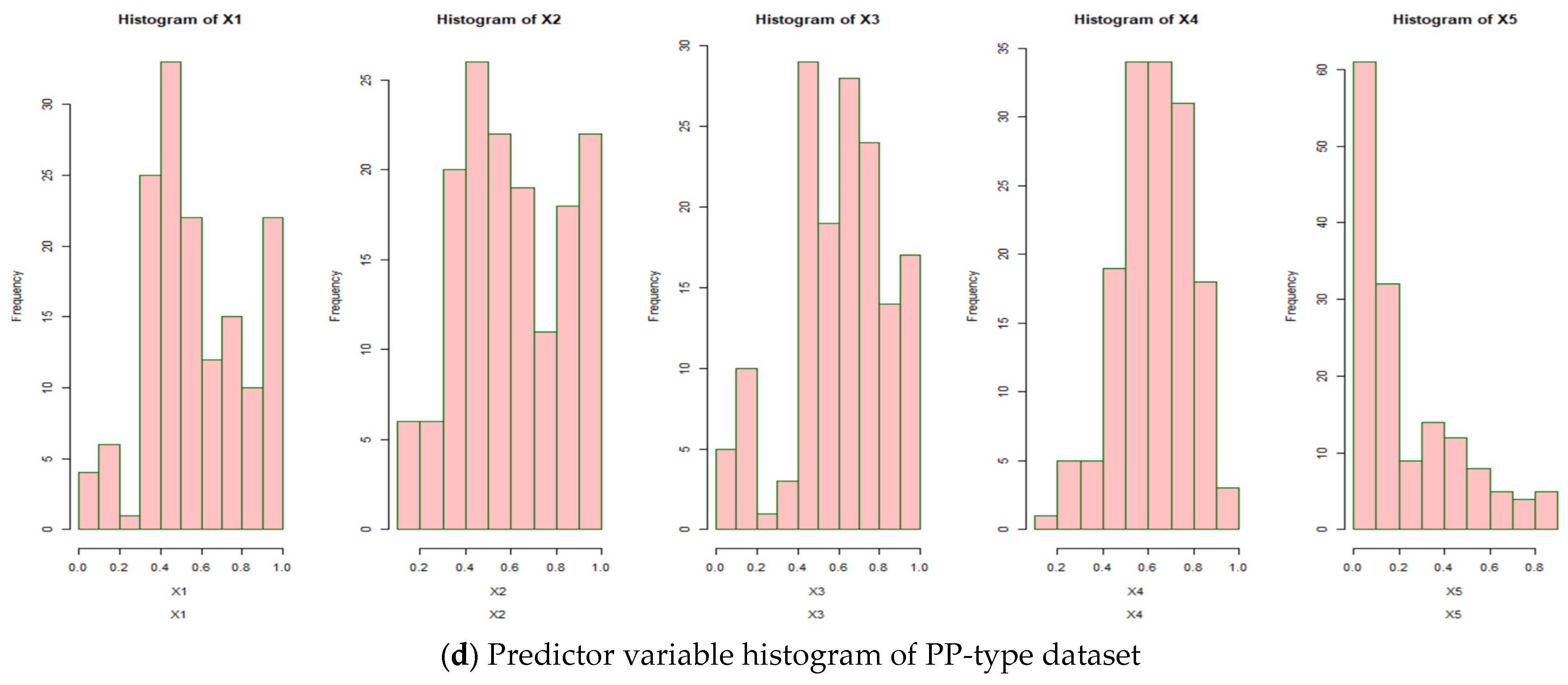
In this work, we suggest an ensemble method constructed from three basic naive Bayes models to predict plastic types. We form one naive Bayes model based on the results of the crisp discretization and two naive Bayes models based on the fuzzy discretization. Each discretization is formed based on antecedent information that the predictor variables obtained from digital image processing are categorized into dark, moderate, and light for each red, green, and blue color channel. The higher the color pixel value in each channel, the lighter the color displayed. The variance and entropy variables are also classified into three categories: low, moderate, and high. A higher value is indicated by a higher number in these two variables.

In the naïve Bayes method, an object or observation is predicted into a specific class based on the maximum posterior probability. The posterior probability is determined according to the Bayes theorem, which is based on the assumption that the predictor variables are independent in a naive (strong) manner.

Let $Y_{j }$be the target variable that denotes the $j$-th class of plastic type, $P\left(Y_j\right)$be the $j$-th class or type prior probability, $P\left(X_1,\cdots ,X_D\left|Y_j\right.\right)$be the likelihood function of the $D$ predictor variables, and $P\left(X_1,\cdots ,X_D\right)$be the joint distribution function of the plastic type. The posterior probability of the plastic type is written as follows [18,22]:

$$\begin{array}{ll}P\left(Y_j\left|X_1,\cdots ,X_D\right.\right)& ={\displaystyle \frac{P\left(Y_j\right)P\left(X_1,\cdots ,X_D\left|Y_j\right.\right)}{P\left(X_1,\cdots ,X_D\right)}}\\ & ={\displaystyle \frac{P\left(Y_j\right)\prod _{d=1}^{D}P\left(X_d\left|Y_j\right.\right)}{\prod _{d=1}^{D}P\left(X_d\right)}}\end{array}$$

(3)

To involve discretization in the naive Bayes method, either crisp or fuzzy discretization, the predictor variables need to be of categorical type, so Equation (3) is adjusted to become Equation (4) [22,36]:

$$P\left(Y_j\left|X_1,\cdots ,X_D\right.\right)={\displaystyle \frac{\sum _{d=1}^{D}n\left(X_d|Y_j\right)+1}{n\left(Y_j\right)+D}}\prod _{d=1}^D{\displaystyle \frac{\sum _k^m{n}_k\left(X_d|Y_j\right)+1}{n\left(X_d|Y_j\right)+m}}$$

(4)

where $n\left(X_d|Y_j\right)$is the amount of plastic images associated to the $j$-th class in all variables $X$, $n\left(Y_j\right)$is the amount of plastic images in the $j$-th class, $n_c\left(X_d|Y_j\right)$is the amount of plastic images associated to the $j$-th class in a variable $X_d$with category $k$, and $m$ is the number of categories in the variable $X_d$.

The $j$-th likelihood function and the $j$-th class or type prior probability, respectively, can be expressed as follows [18,22,36]:

$$P\left(X_d\left|Y_j\right.\right)={\displaystyle \frac{\sum _k^m{n}_k\left(X_d|Y_j\right)+1}{n\left(X_d|Y_j\right)+m}}$$

(5)

$$P\left(Y_j\right)={\displaystyle \frac{\sum _{d=1}^{D}n\left(X_d|Y_j\right)+1}{n\left(Y_j\right)+D}}$$

(6)

The following assumptions are needed to integrate fuzzy discretization into naive Bayes. Suppose ${\tilde{X}}_d=\left\{x_{f_1}, x_{f_1}\cdots ,x_{f_Z}\right\}$is the fuzzy sample information space of the red, green, and blue as predictor variables of $X_d$, $x_{f_z}\in X$is the independent event, and ${\mu }_{{\tilde{X}}_d}\left(x_{f_z}\right)$is the fuzzy membership function of $X_d$, then the fuzzy sample conditional probability function is formulated as $P\left({\tilde{X}}_d|Y_j\right)=\sum _{z=1}^{Z}P\left(x_{f_z}|Y_j\right){\mu }_{{\tilde{X}}_d}\left(x_{f_z}\right)$, and the prior probability of the predictor variable is $P\left({\tilde{X}}_d\right)=\sum _{z=1}^{Z}P\left(x_{f_z}\right){\mu }_{{\tilde{X}}_d}\left(x_{f_z}\right)$. Since the evidence is not fixed in the fuzzy set and the Laplace smoothing effect, the posterior probability is as follows [22,39]:

$$\begin{array}{ll}P\left(Y_j\left|X_1,\cdots ,X_D\right.\right)& = {\displaystyle \frac{P\left(Y_j\right)\prod _{d=1}^{D}P\left({\tilde{X}}_d|Y_j\right)}{\prod _{d=1}^{D}P\left({\tilde{X}}_d\right)}}\\ & = {\displaystyle \frac{P\left(Y_j\right)\prod _{d=1}^D\sum _{z=1}^{Z}P\left(x_{f_z}|Y_j\right){\mu }_{{\tilde{X}}_d}\left(x_{f_z}\right)+\frac{1}{Z}}{\prod _{d=1}^D\sum _{z=1}^{Z}P\left(x_{f_z}\right){\mu }_{{\tilde{X}}_d}\left(x_{f_z}\right)+\frac{1}{Z}}}\end{array}$$

(7)

The development of the naive Bayes model using fuzzy discretization includes two different combinations of fuzzy membership functions. First, a combination of triangular functions and linear functions (decreasing, increasing). Second, a combination of trapezoidal functions and linear functions (also decreasing and increasing). In both combinations, decreasing and increasing linear functions are used to discretize the first and third categories for each predictor variable, while triangular and trapezoidal functions are used to discretize the second category in each combination. The fuzzy membership functions are presented in Equations (8)–(11).

Assume that $a$ is the least conspicuous domain entry with a membership value of 1, and b is the most conspicuous domain entry with a membership value of 0. The decreasing linear function is expressed as follows [22,40]:

$${\mu }_{{\tilde{X}}_d}\left(x_f;a,b\right)=\left\{\begin{array}{c}1 x_f\le a\\ {\displaystyle \frac{b-x_f}{b-a}} a\le x_f\le b\\ 0 x_f\ge b\end{array}\right.$$

(8)

Let $a$be the least conspicuous domain entry with a membership value of 0, and b be the most conspicuous domain entry with a membership value of 1. The increasing linear function can be written as follows [22,40]:

$${\mu }_{{\tilde{X}}_d}\left(x_f;a,b\right)=\left\{\begin{array}{c}0 x_f\le a\\ {\displaystyle \frac{x_f-a}{b-a}} a\le x_f\le b\\ 1 x_f\ge b\end{array}\right.$$

(9)

For the triangular membership function, assume that $a$ is the least conspicuous domain entry with a membership value of 0, $b$ is a domain entry with a membership value of 1, and $c$ is the most conspicuous domain element with a membership value of 0. The function can be formulated as follows [22,29,41]:

$${\mu }_{{\tilde{X}}_d}\left(x_f;a,b,c\right)=\left\{\begin{array}{c}0 x_f\le a\\ {\displaystyle \frac{x_f-a}{b-a}} a\le x_f\le b\\ {\displaystyle \frac{c-x_f}{c-b}} b\le x_f\le c\\ 0 x_f\ge c\end{array}\right.$$

(10)

Let $a$ be the least conspicuous domain entry with a membership value of 0, $b$ be a domain entry with a membership value of 1, $c$ be a domain entry with a membership value of 1, and $d$ be the most conspicuous domain entry with a membership value of 0. The trapezoidal membership function is represented as follows [22,41]:

$${\mu }_{{\tilde{X}}_d}\left(x_f;a,b,c,d\right)=\left\{\begin{array}{c}0 x_f\le a\\ {\displaystyle \frac{x_f-a}{b-a}} a\le x_f\le b\\ 1 b\le x_f\le c\\ {\displaystyle \frac{d-x_f}{d-c}} c\le x_f\le d\\ 0 x_f\ge d\end{array}\right.$$

(11)

In the machine learning concept, the prediction model performance is validated for unseen data, so the data must be split into training or modeling and test data. This research applied the k-fold cross-validation with k = 5 in the split dataset. The dataset was randomly separated into five folds of similar size, with one fold allocated as testing data and the remaining four assigned as modeling data. Each of the five iterations contained distinct data compositions for modeling and testing with a ratio of 80:20. The final model performance was the average of the five iterations [42,43]. The 5 fold was less biased compared to other numbers of folds [44] and capable of evaluating the quality and the stability of the model as well as preventing overfitting without reducing the quantity of learning data used [42].

The ensemble prediction model performance was then tested to obtain prediction results, as are all basic models. Let ${\mathrm{T}\mathrm{P}}_j$ be the true positive prediction at $j$-th class, ${\mathrm{T}\mathrm{N}}_j$ be the true negative prediction at $j$-th class, ${\mathrm{F}\mathrm{P}}_j$ be the false positive prediction at $j$-th class, and ${\mathrm{F}\mathrm{N}}_{j }$be the false negative prediction at $j$-th class. For the first class, all of the true and the false predictions are given in

Table 1. Confusion matrix for the first class.

	$\mathit{j}$	Prediction
		1	2	3
	1	${\mathrm{T}\mathrm{P}}_j$	${\mathrm{F}\mathrm{P}}_j$	${\mathrm{F}\mathrm{P}}_j$
Actual	2	${\mathrm{F}\mathrm{N}}_j$	${\mathrm{T}\mathrm{N}}_j$	${\mathrm{T}\mathrm{N}}_j$
	3	${\mathrm{F}\mathrm{N}}_j$	${\mathrm{T}\mathrm{N}}_j$	${\mathrm{T}\mathrm{N}}_j$

, and the other classes can be found similarly.

The evaluation metrics of model performance for $J$ classes of plastic type are given in (12)–(14) [20,45].

$$\mathrm{A}\mathrm{c}\mathrm{c}\mathrm{u}\mathrm{r}\mathrm{a}\mathrm{c}\mathrm{y}={\displaystyle \frac{\sum _{j=1}^J\frac{{\mathrm{T}\mathrm{P}}_j+{\mathrm{T}\mathrm{N}}_j}{{\mathrm{T}\mathrm{P}}_j+{\mathrm{F}\mathrm{P}}_j+{\mathrm{F}\mathrm{N}}_j+\mathrm{T}\mathrm{N}}}{J}}$$

(12)

$$\mathrm{P}\mathrm{r}\mathrm{e}\mathrm{c}\mathrm{i}\mathrm{s}\mathrm{i}\mathrm{o}\mathrm{n}={\displaystyle \frac{\sum _{j=1}^J\frac{{\mathrm{T}\mathrm{P}}_j}{{\mathrm{T}\mathrm{P}}_j+{\mathrm{F}\mathrm{P}}_j}}{J}}$$

(13)

$$\mathrm{R}\mathrm{e}\mathrm{c}\mathrm{a}\mathrm{l}\mathrm{l}= {\displaystyle \frac{\sum _{j=1}^J\frac{{\mathrm{T}\mathrm{P}}_j}{{\mathrm{T}\mathrm{P}}_j+{\mathrm{F}\mathrm{N}}_j}}{J}}$$

(14)

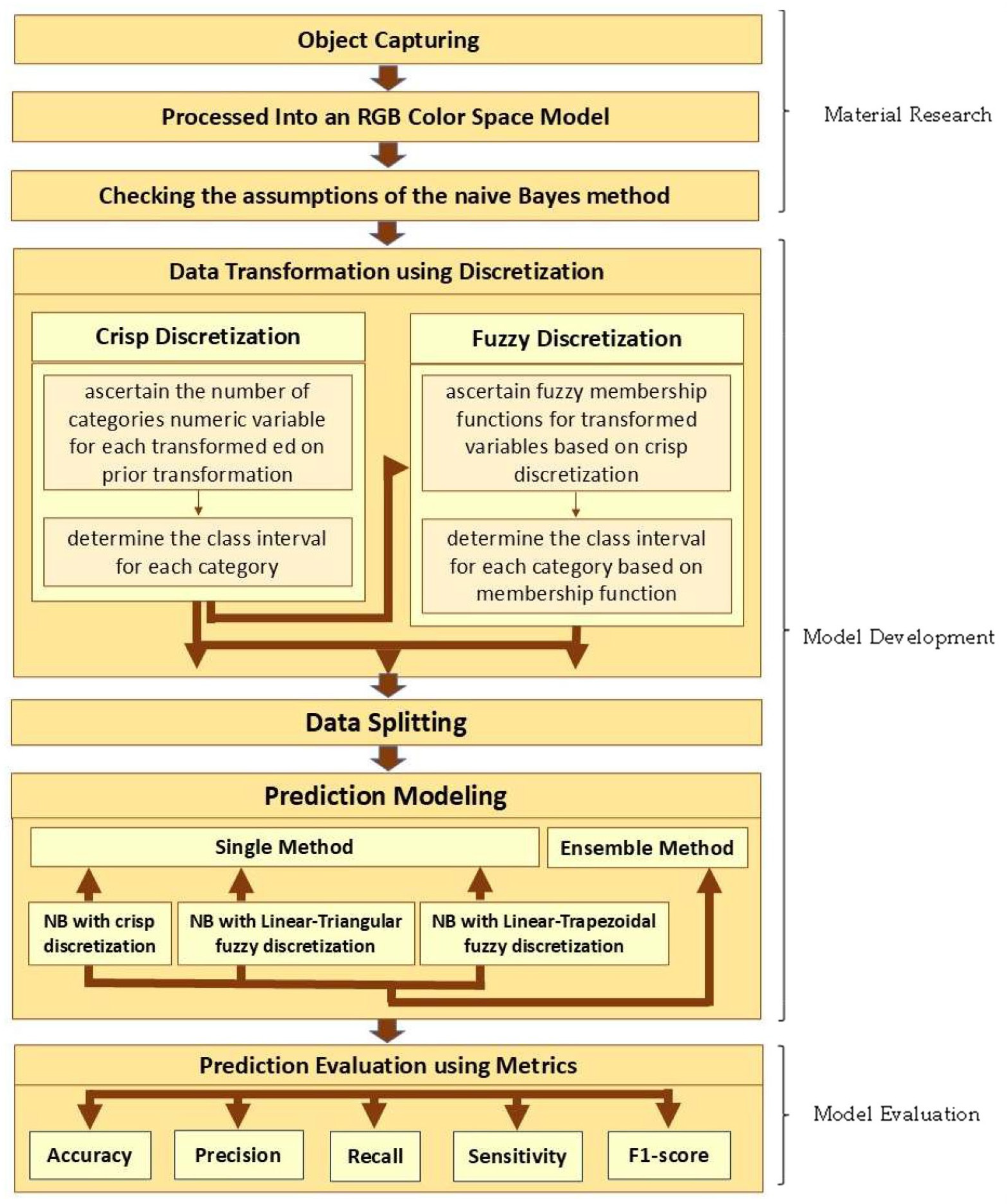
A satisfactory prediction performance is indicated by the highest metric size. In general, the research steps are described in Figure 2.

3. Results and Discussion

The five components of image processing in the chromatic model of RGB are red, green, and blue color channels as well as entropy and variance that are used as predictor variables and denoted by $X_1, X_2,X_3,X_4,$ and $X_5,$ successively.

The summary of the predictor variables after rescale into 0–1, as represented in Figure 3, shows that some variables have a minimum value of zero and not all variables have a maximum value of 1 (with rounding to two decimal places). HDPE type has the highest mean value for all variables, except for variable $X_4$, which is the smallest compared to the other classes. The lowest maximum value is owned by variable $X_5$ in the PP type.

Assessing the Pearson correlation is helpful to show that the naïve assumption between predictor variables in the naïve Bayesian method is met. As presented in Figure 4, in the overall data, the majority of correlations are high (more than 0.7), indicating a strong linear relationship, both positive and negative [46]. In both plastic types PET and HDPE, in addition to having a majority of high correlations, there are also very high (very strong) correlations. In the PP type, although the majority of correlations are low, there is one high correlation, namely the correlation between variables $X_2$ and $X_5$.

Assessing the Gaussian assumption is helpful to show that the assumptions in the naïve Bayesian method for numeric predictor variables in the case of this study are not met; therefore, the discretization of predictor variables is indeed feasible, so the naïve Bayes method can be used. The histograms for each predictor variable are presented in Figure 4. All variables in Figure 5a,b show excessive skewness because they have two peaks in two different locations (bimodal). In Figure 5c, the preponderance of the variable distribution skews to the left (the median is greater than the mean), $X_4$ only tends to be skewed to the right (the median is smaller than the mean), and a bimodal distribution is prevalent for $X_5$. In Figure 5d, the distribution of $X_5$ is biased to the right, whereas the other three variables are characteristically bimodal. This fact shows that, both in the data as a whole and for each plastic type, all are not Gaussian distributed, except for variable $X_4$ in the PP type.

Since the assumptions of the naïve Bayes method for numeric variables are not met, the discretization of predictor variables proposed in this work is feasible. Crisp discretizes that all predictor variables of the plastic-type dataset can be assigned to three categories based on antecedent information [18], where previously, the data were rescaled into values 0–1 to have uniform units. The crisp discretization parameters are obtained using Equation (1) [23,36].

In the crisp discretization, as presented in

Table 2. Crisp discretization.

	Predictor Variable	Category $\left(\mathit{m}\right)$
		1	2	3
Crisp Discretization Parameter	$X_1$	[0.329, 0.553]	[0.554, 0.776]	[0.777, 1]
	$X_2$	[0.350, 0.567]	[0.568, 0.783]	[0.784, 1]
	$X_3$	[0.330, 0.553]	[0.554, 0.776]	[0.777, 1]
	$X_4$	[0, 0.333]	[0.334, 0.667]	[0.668, 1]
	$X_5$	[0, 0.039]	[0.040, 0.082]	[0.083, 1]

, each $m$-th category in each predictor variable has only two parameters, which are the lower and upper classes limits and do not overlap. The results of this crisp discretization are then implemented in the naïve Bayes method to predict three plastic types, both as a single method and in building an ensemble method. Fuzzy discretization for both linear–triangular combinations and linear–trapezoidal function combinations is formed based on crisp discretization. The parameters of both fuzzy discretization combinations are obtained using tuning systems [23,24]. The results of both fuzzy discretization models are shown in

Table 3. Linear–triangular fuzzy discretization.

	Predictor Variable	Category $\left(\mathit{m}\right)$
		1	2	3
Fuzzy Discretization Parameter	$X_1$	[0.329, 0.776]	[0.553, 0.948, 0.944]	[0.888, 1]
	$X_2$	[0.350, 0.783]	[0.567, 0.656, 0.946]	[0.892, 1]
	$X_3$	[0.330, 0.776]	[0.553, 0.748, 0.944]	[0.888, 1]
	$X_4$	[0, 0.667]	[0.333, 0.625, 0.916]	[0.833, 1]
	$X_5$	[0, 0.082]	[0.039, 0.295, 0.552]	[0.104, 1]

and

Table 4. Linear–trapezoidal fuzzy discretization.

	Predictor Variable	Category $\left(\mathit{m}\right)$
		1	2	3
Fuzzy Discretization Parameter	$X_1$	[0.329, 0.776]	[0.553, 0.751, 0.944, 0.948]	[0.888, 1]
	$X_2$	[0.350, 0.783]	[0.567, 0.711, 0.656, 0.946]	[0.892, 1]
	$X_3$	[0.330, 0.776]	[0.553, 0.651, 0.748, 0.944]	[0.888, 1]
	$X_4$	[0, 0.667]	[0.333, 0.479, 0.625, 0.916]	[0.833, 1]
	$X_5$	[0, 0.082]	[0.039, 0.167, 0.295, 0.552]	[0.104, 1]

, respectively.

Table 3 shows that the first and third categories only have two parameters because the membership functions used are descending and increasing linear functions. However, the second category has three parameters because the membership functions used are triangular functions. Like crisp discretization, the results of this linear–triangular fuzzy discretization are then implemented in the naïve Bayes method to predict three plastic types, both as a single method and in building an ensemble method.

In Table 4, the first and third categories in this fuzzy discretization also use descending and increasing linear functions so that they only have two parameters, but the second category has four parameters because it follows the membership function used, namely the trapezoidal function. The results of this linear–trapezoidal fuzzy discretization are then implemented in the naïve Bayes method to predict three plastic types, both as a single method and in building an ensemble method.

Small disturbances or changes in training data often affect the performance of the prediction. Consequently, it is imperative to generalize the model’s performance to reflect the actual performance of the model. We propose different random resampling in dividing the folds in k-fold cross-validation to generalize the basic model performance and the performance of the proposed ensemble of triple naive Bayes models, which is the average of the performance of all resampling [33]. To accommodate the use of ANOVA and ad hoc tests, resampling is performed more than 30 times (exactly 35 times).

The results of the prediction of objects into specific classes for the first sampling of 5-fold cross-validation using NB with crisp discretization and two models using NB with fuzzy discretization as a single method and also the ensemble method are summarized in the confusion matrix shown in

Table 5. Confusion matrix of four proposed NB.

(a) NB with Crisp Discretization
		Prediction
	Plastic Type	PET	HDPE	PP	Sum
Actual	PET	26	0	0	26
	HDPE	2	30	2	34
	PP	0	0	30	30
	Sum	28	30	32	90
(b) NB with Linear–Triangular Fuzzy Discretization
		Prediction
	Plastic Type	PET	HDPE	PP	Sum
Actual	PET	23	3	0	26
	HDPE	0	32	2	34
	PP	0	0	30	30
	Sum	23	35	32	90
(c) NB with Linear–Trapezoidal Fuzzy Discretization
		Prediction
	Plastic Type	PET	HDPE	PP	Sum
Actual	PET	22	4	0	26
	HDPE	0	32	2	34
	PP	0	0	30	30
	Sum	22	36	32	90
(d) Ensemble of Triple Naïve Bayes
		Prediction
	Plastic Type	PET	HDPE	PP	Sum
Actual	PET	26	0	0	26
	HDPE	0	32	2	34
	PP	0	0	30	30
	Sum	26	32	32	90

. From this table, metrics can be determined that show prediction performance.

In the first sampling, the test data, which are one-fold, contain 80% of the data (90 observations) and are distributed into PET, HDPE, and PP plastic types of 26, 34, and 30, respectively. The distribution of observations in the training data and test data to each plastic type can vary in each resampling.

The performance metrics of predictions in the first sampling of 5-fold cross-validation using NB with crisp discretization, two NB models with fuzzy discretization, and the ensemble method built from the three single NB models are presented in

Table 6. Performance metrics on the first resampling for single and ensemble model.

Model	Performance Metric
	Accuracy	Precision	Recall
NB with crisp discretization	95.56	95.54	96.08
NB with linear–triangular fuzzy discretization	94.44	95.06	94.19
NB with linear–trapezoidal fuzzy discretization	93.33	94.21	92.91
Ensemble of triple NB	97.78	97.92	98.04

.

Among the three basic models, the highest model performance in the first sampling of 5-fold cross-validation is owned by the NB model with crisp discretization, while the lowest is owned by the NB model with linear–trapezoidal discretization. The ensemble of the triple NB model exhibits the highest performance compared to the other three basic models in accuracy, precision, and recall, with a percentage of 97.78–98.04%.

Furthermore, the performance of these models cannot be generalized, considering that each sampling can provide different prediction performance as presented in Figure 6. The figure shows that the four proposed models have different performances in each random resampling of 5-fold cross-validation technique. The twenty-seventh resampling in the NB model with crisp discretization exhibits the lowest performance, with accuracy, precision, and recall ranging from 91% to 92%. However, the highest performance is at the fifth resampling, which reaches 100% for all metrics. Similar events also occur in the performance of the two models of NB with fuzzy discretization. The lowest and highest performances for the linear–triangular combination are at the eighth and thirty-first resampling, respectively, with metric values ranging from 86 to 87% and 97 to 98%. In the linear–trapezoidal combination, the lowest and highest performances are at the eighth and thirty-third resampling, respectively, with metric values ranging from 85 to 87% and 97 to 98%. Similar to the performance of the three single NB prediction models, the ensemble model also has different performances in each resampling.

Table 7. Performance generalization for single and ensemble of triple NB model.

Model	Performance Metric (%)
	Accuracy	Precision	Recall
NB with crisp discretization	95.05	95.16	94.92
NB with linear–triangular fuzzy discretization	92.63	93.32	92.61
NB with linear–trapezoidal fuzzy discretization	91.59	92.51	91.51
Ensemble of triple NB	97.11	97.30	97.07

presents three critical pieces of information regarding the performance generalization of the four proposed models, which are based on the thirty-five resampling. First, among the three proposed single methods, the performance of the NB with crisp discretization and NB with linear–trapezoidal fuzzy discretization models is the highest and the lowest, respectively. Second, the ensemble model built from the three single NB models, which have performances in the range of 91.51–95.16%, has a performance in the range of 97.07–97.3%. Third, the performance improvement of the ensemble model compared to each single model with NB with crisp discretization, NB with linear–triangular, and NB with linear–trapezoidal is 2.06–2.15%, 3.98–4.49%, and 4.79–5.56%, respectively.

This fact also informs us that fuzzy discretization does not always provide better performance than crisp discretization. It is suspected that the crisp discretization that is carried out does not produce vagueness in each category of the variable. However, the performance of the plastic-type prediction model using the NB model with discretization, which has the highest performance among the proposed single models, can be improved through the ensemble method, which is built from a combination of crisp and fuzzy discretization models.

Additionally, ANOVA (

Table 8. ANOVA of single and ensemble methods.

Metrics	Source of Var.	Sum of Squares	Mean Squares	F	p-Value	F-Criteria
Accuracy	between	0.06	0.02	40.98	6.25 × 10−19	2.67
	within	0.07	0.00
Recall	between	0.07	0.02	45.84	1.71 × 10−20
	within	0.06	0.00
Precision	between	0.05	0.02	38.28	5.34 × 10−18
	within	0.06	0.00

) shows whether the four proposed models’ performance is distinct, and when using the proposed ensemble models, whether the performance metrics have improved significantly.

The ANOVA demonstrates that the four proposed models show a significant improvement in performance metrics at 5% significance levels as well as a difference in at least one average performance metric for accuracy, precision, and recall. A post hoc test employing the Tukey–Kramer test is illustrated in

Table 9. Tukey–Kramer test of single and ensemble methods.

Comparison Model	Absolute Mean Difference
	Accuracy	Recall	Precision
NB with crisp discretization vs. NB with linear–triangular	0.02	0.02	0.02
NB with crisp discretization vs. NB with linear–trapezoidal	0.03	0.03	0.03
NB with crisp discretization vs. ensemble of triple NB	0.02	0.02	0.02
NB with linear–triangular vs. NB with linear–trapezoidal	0.01	0.01	0.01
NB with linear–triangular vs. ensemble of triple NB	0.04	0.04	0.04
NB with linear–trapezoidal vs. ensemble of triple NB	0.06	0.05	0.06

.

The Absolute Mean Difference (AMD) between the two models is more than the Q-critical value, which results in a significant increase in metrics. The critical values for all three metrics in this study are 0.01. All three metrics have a substantial difference between all model pairings. This fact also indicates that the performance of the triple NB ensemble model is substantially better than that of all single NB models. The ensemble model’s efficacy is also influenced by the combination of the single models that have been constructed. Statistical tests that substantiate the research hypothesis demonstrate that the proposed prediction model, which is constructed from three naive Bayes models, performs exceptionally well and is exceedingly robust.

4. Comparison with Other Studies

Several other works that build intelligent computing systems for sorting plastic waste based on machine learning are presented in

Table 10. Comparison with other studies.

Paper	Plastic Type	Dataset	Sum of Sample	The Best Prediction Method Used	Validation Method	Performance Generalization	Metric Performance (%)
							Accuracy	Recall	Precision
Choi et al. [4]	PET and PET-G	Image sensor and deep learning You Only Look Once (YOLO)	-	-	-	-	45.50	47.64	91.00
Shi et al., [7]	Colorless, light blue, light green, and apple green transparent plastics of PET	Multi-wavelength transmission spectrum	40	Naïve Bayes	10-fold cross-validation	-	100.00	100.00	100.00
Singh et al. 2023 [12]	PET, HDPE, PP, PS	Hyperspectral image in near-infrared	20	Artificial Neural Network	hold out 80:20	-	87.00	87.33	87.15
Bonifazi et al. [13]	Electric and Electronic Equipment (WEEE)	Hyperspectral image in Short-Wave InfraRed (SWIR) spectral	-	Partial Least Squared-Linear Discriminant Analysis	-	-		86.7
Martinez-Hernandez et al. [14]	PET, HDPE, PVC, LDPE, PP, and PS	Triad Spectroscopy Sensor	423	Convolutional Neural Network with Principal Component Analysis	10-fold cross-validation	-	72.50	72.50	72.43
Yani and Resti, 2024 [18]	PET, HDPE, PP	RGB image	450	Multinomial Naïve Bayes	5-fold cross-validation	-	97.34	96.00	-
Yani et al. [20]	PET, HDPE, PP	RGB image	450	Fisher Discriminant Analysis			87.11	91.67	-
Proposed Method	PET, HDPE, PP	RGB image	450	Ensemble of Triple naïve Bayes	5-fold cross-validation	thirty-five resampling of 5-fold cross-validation	97.11	97.30	97.07

as a comparison. The majority of the works use the validation method using k-fold cross-validation. In work [4], the precision metric that describes the percentage of objects that are truly the actual plastic type from all objects predicted as that type is high, which is more than 90%. Nevertheless, the accuracy, which is defined as the proportion of observations that are accurately classified in all plastic varieties, is low at 45.5%. Likewise, the recall that describes the percentage of observations in a plastic type that are successfully predicted as the same plastic type shows a low value (47.64%). The work also does not use a validation method in performing its prediction task. In work [12], which validates the prediction performance using 10-fold cross-validation and obtains a performance of 100%, in addition to not being generalized, the number of samples of 20 indicates that the test data of only four allow for as many true predictions as the test data so that the performance metric easily achieves 100%. Consequently, the model’s efficacy is also influenced by the quantity of samples. We have shown that the performance of k-fold cross-validation can be different in each sampling, as given in Figure 6; therefore, it is necessary to generalize the performance of the prediction model built for a machine learning-based system of at least thirty samplings [33]. The difference between the method we propose and the current method is that the ensemble method we propose is built from single methods in the form of NB methods that implement discretization, both crisp and fuzzy. Our proposed method has also proposed generalization to the performance of all proposed models, both the single NB method and the ensemble of the triple NB method, and obtained satisfactory performance (more than 97%).

According to [47,48,49], a performance above 85% is considered satisfactory. We built an intelligent computing system that has high, stable, and robust performance, as proven using statistical tests presented in Table 8, with accuracy, precision, and recall metric indicators all above 97% (Table 7). The main advantage of using our proposed method with high, stable, and robust performance is that the automatic plastic sorting process can run effectively and efficiently. The industry can use this resulting method to build automatic sorting computations.

5. Conclusions

The novelty of this study is to build intelligent computing using an ensemble model based on three single NB models to predict three types of plastic. The three basic models consist of one NB model with crisp discretization and two NB models with fuzzy discretization, namely those using a combination of fuzzy linear–triangular membership functions and a combination of fuzzy linear–trapezoidal membership functions. Five-fold cross-validation was employed to validate each proposed model, and thirty-five times resampling was employed to generalize it. The efficacy of the NB model with fuzzy discretization is influenced by the combination of fuzzy membership functions that are employed. The performance of the NB model with imprecise discretization is not superior to that of the NB model with crisp discretization. The hypothesis that the ensemble model outperforms all individual models and that the performance of the four proposed NB-based models differs in at least one metric has been validated. The four proposed models demonstrate a performance improvement from the single method to the ensemble method of the triple naive Bayes, with a range of 2.06% to 5.56%, as evidenced by a generalization of performance based on some resampling of five-fold cross-validation. Furthermore, the proposed prediction model’s robust and high performance is demonstrated by the evidence supporting this hypothesis, which is constructed from three naive Bayes models using the ensemble method. No prediction method is effective for all cases, and neither is the proposed ensemble method. The implementation of discretization, especially fuzzy, is influenced by many factors, such as the number of categories, types of functions, and combinations of fuzzy membership functions. Likewise, the ensemble method, built from naive Bayes methods with fuzzy discretization, is influenced not only by fuzzy discretization but also by the combination of single methods that build it. Further exploration is necessary. Furthermore, this research is also expected to be continued for other types of plastic that have not been discussed in this study.