Abstract
Land Surface Temperature (LST), as a core variable in the coupling of land–atmosphere energy transfers and ecological responses, relies heavily on the global coverage capacity of thermal infrared remote sensing (TIR-LST) for dynamic monitoring. Currently, the time reconstruction method of the TIR-LST products from China’s Fengyun polar-orbiting satellite under dynamic cloud interference remains under exploration. This study focuses on the Heihe River Basin in western China, and addresses the issue of cloud coverage in relation to the Fengyun-3C (FY-3C) satellite TIR-LST. An innovative spatiotemporal reconstruction framework based on multi-source data collaboration was developed. Using a hybrid ensemble learning framework of random forest and ridge regression, environmental parameters such as vegetation index (NDVI), land cover type (LC), digital elevation model (DEM), and terrain slope were integrated. A downscaling and multi-factor collaborative representation model for land surface temperature was constructed, thereby integrating the passive microwave LST and thermal infrared VIRR-LST from the FY-3C satellite. This produced a seamless LST dataset with 1 km resolution for the period of 2017–2019, with temporal continuity across space. The validation results show that the reconstructed data significantly improves accuracy compared to the original VIRR-LST and demonstrates notable spatiotemporal consistency with MODIS LST at the daily scale (annual R2 ≥ 0.88, RMSE < 2.3 K). This method successfully reconstructed the FY-3C satellite’s 1 km level all-weather LST time series, providing reliable technical support for the use of domestic satellite data in remote sensing applications such as ecological drought monitoring and urban heat island tracking.
1. Introduction
Land Surface Temperature (LST) is a key parameter for understanding the physical and chemical interactions between a land surface and atmosphere, and plays a crucial role in several priority research areas of the International Geosphere-Biosphere Programme (IGBP), such as drought monitoring, evapotranspiration assessment, soil moisture determination, urban heat island effect detection, and global climate change analysis [1,2,3,4]. In these fields, accurate, continuous, and comprehensive LST data are essential for research. However, the traditional methods of obtaining surface temperature, especially those relying on thermal infrared sensors, are often limited by cloud cover [5,6,7], making it difficult to provide continuous all-weather monitoring. This limitation has driven the exploration and development of reliable all-weather LST retrieval methods, highlighting the urgent need for new research directions and technological innovations. Microwave (PMW) radiation can penetrate cloud cover, but it has a relatively lower spatial resolution [8]. Therefore, it is evident that TIR and PMW have complementary spatial layouts and data accuracy. As a result, the fusion of TIR and PMW data has become a promising approach for obtaining high-quality, complete LST data [9,10].
To date, traditional fusion methods for TIR and PMW include the Bayesian Maximum Entropy (BME) method by Xu, Cheng, and Zhang [11], temperature spatial interpolation used by Duan and Sun [12,13], cloud proportion weighting [14], and time component decomposition by Zhang [15]. Most traditional methods yield high-precision LST fusion results; however, they all have limitations. For instance, the cloud proportion weighting method may suffer from reduced accuracy and instability when cloud cover is extensive. The temperature spatiotemporal interpolation method can result in significant interpolation errors when data distribution is uneven and has high computational complexity. The time component decomposition method is heavily dependent on historical data, with a complex model that is difficult to adjust. The BME method is computationally demanding and requires stringent probability assumptions.
The limitations of these traditional methods make them less applicable in large-scale and high-precision scenarios. In contrast, machine learning methods [16,17] are more capable of handling complex data processing and analysis tasks due to their superior performance and versatility. Machine learning and deep learning techniques, with their ability to model complex data relationships, provide promising new approaches for all-weather LST prediction. Although these methods require more computational resources, they excel at identifying underlying patterns, capturing nonlinear relationships, and delivering precise predictions.
To address the technical challenges in this field, this study proposes an innovative machine learning-based method for generating all-weather LST, which fully leverages the potential of domestic Fengyun-3C satellite data [18]. This method is the first to combine Fengyun satellite data, including vegetation index, infrared temperature, and microwave temperature, for surface temperature reconstruction. Unlike previous studies that typically used high-resolution satellite data such as MODIS and Sentinel, this experiment relies entirely on Fengyun satellite data, aiming to explore the potential of this dataset. This represents a novel approach in terms of the data used. Additionally, the SSA method was applied to fill orbital gaps in the microwave and infrared data, further enhancing the novelty of the experimental methodology. Moreover, a stacked model, rather than a single model, was employed for training, highlighting another innovative aspect of the approach. The novel approach integrates the Ridge Regression and Random Forest ensemble algorithm, with the two methods complementing each other. Ridge regression, proposed by Hoerl and Kennard [19], is robust in handling multicollinearity issues, making it suitable for large-scale regression analysis. The Random Forest model, introduced by Breiman [20], is a widely used method in machine learning that builds multiple decision trees to enhance the model’s tolerance to randomness and predictive capability. The stacked model of these two methods demonstrates outstanding performance in providing all-weather LST, particularly in areas with frequent cloud cover, offering a new and reliable data source for global climate change research and environmental monitoring.
This paper further outlines the scientific foundation, experimental design, and detailed construction process of the novel all-weather LST generation method. Through a comprehensive introduction to the study area and data, as well as an in-depth analysis and discussion of the model results, the paper thoroughly elaborates on the theoretical value and practical application potential of this research. Finally, by summarizing the conclusions, the paper highlights the feasibility and innovation of the all-weather surface temperature reconstruction method based on FY-3C data in the field of remote sensing technology.
2. Study Area and Data
2.1. Study Area
This study focuses on the Heihe River basin [21] in the northwestern part of China. The region is geographically located between approximately 98° E to 105° E and 37° N to 42° N, and is a typical inland river basin, as shown in Figure 1.
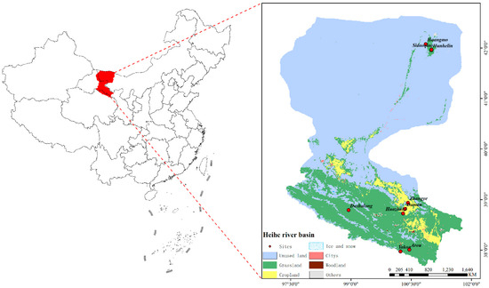
Figure 1.
Heihe District Division Map and location distribution of sites.
China’s geographic environment is complex, characterized by significant elevation differences, diverse land cover types, and a wide range of climate types. The Heihe River region exhibits a similarly intricate geographic environment, including Deserts, Grasslands, and Farmland. The climate is varied, ranging from arid to semi-arid, making it an ideal location for studying surface temperature variations. Based on the image, it can be observed that a significant portion of the Heihe River Basin consists of unused land, which refers to areas where more than 60% of the surface is devoid of vegetation, with vegetation cover below 10%. Due to the lack of vegetation’s shielding and cooling effects, these barren lands exhibit higher absorption and reflection of radiation rates, leading to higher surface temperatures in the region. High spatial resolution LST holds immense value across various applications, and TIR LST products are currently the most widely used high-resolution LST. However, TIR LST is highly susceptible to cloud and fog interference, leading to significant data loss under cloudy conditions. For example, the MODIS LST product shows extensive data loss across China. Therefore, developing an all-weather LST generation method suited for China and obtaining spatially seamless, high-resolution TIR LST are of considerable practical significance.
2.2. Data
The data used in this study are divided into two categories: satellite data and site validation data. To ensure an adequate number of validation sites and the temporal integrity of satellite data, the study period was selected to span from 2017 to 2019. The detailed data are listed in Table 1 and Table 2.

Table 1.
Basic information of the datasets used in this study.
Table 2.
Validation site information.
2.2.1. Satellite Data
The Visible and Infrared Radiometer (VIRR) aboard the Fengyun-3C (FY-3C) satellite was developed by the China Meteorological Administration (CMA) and is operated by the National Satellite Meteorological Center (NSMC) in Beijing, China. VIRR LST is one of the most commonly used TIR LST products in China, with a spatial resolution of 1 km and a temporal resolution of daily. VIRR LST is a TIR LST product retrieved using a windowing algorithm, offering high spatial resolution and accuracy, making it a reliable data source for surface temperature monitoring. Additionally, the VIRR LST will show “NoData” values in areas with cloud coverage, which makes it easier to identify and check for cloud-covered pixels in the experiment. Therefore, this study uses VIRR LST as the primary component for generating all-weather LST. In addition, VIRR NVI (Normalized Vegetation Index, NDVI) and MCD12Q1 land cover (LC) data are selected as auxiliary data for the all-weather surface temperature generation process. The spatial resolution of VIRR NVI is 5 km, with a temporal resolution of 10 days. To match the temporal resolution of VIRR LST, this study applies a time interpolation method based on Savitzky–Golay filtering to the VIRR NVI, generating daily NDVI products. The MCD12Q1 LC used in this study is a land cover product based on the IGBP global vegetation classification scheme. It has a spatial resolution of 500 m and a temporal resolution of once per year.
To generate all-weather LST based on the VIRR LST dataset, several additional variables were incorporated, including seamless spatial PMW LST, digital elevation model (DEM), longitude and latitude, and slope. The spatially seamless PMW LST dataset used in this study comes from the processed MWRI LST, which is a surface temperature product from the Microwave Radiation Imager (MWRI). MWRI LST has a spatial resolution of 25 km and a temporal resolution of one day. However, it is affected by orbital constraints, resulting in parts of the images being blocked by the orbit. To address this, a time-series analysis method based on a Singular Spectrum Analysis (SSA) was employed to interpolate the missing regions. To match the spatial resolution of VIRR LST, machine learning methods were used to downscale the interpolated MWRI LST data. The DEM data obtained from the Shuttle Radar Topography Mission (SRTM) and the slope data derived from the DEM both have a spatial resolution of 900 m.
2.2.2. Site Validation Data
To assess the accuracy of the generated all-weather surface temperature, field measurement data from the Heihe River Basin Integrated Remote Sensing Experiment (HiWATER) project [22,23] in the Heihe River Basin were collected. These data can be downloaded from the National Tibetan Plateau Data Center (http://www.tpdc.ac.cn/zh-hans/data (accessed on 23 March 2024)). The datasets include four-component radiation, surface radiative temperature, soil heat flux, and other observational data, which were collected from ground-based observation stations. Four-component radiation is measured by the CNR4 net radiometer, with a maximum nonlinear error of 1%. The in situ surface temperature, calculated from upward and downward longwave radiation based on four-component radiation, has been widely used to validate the accuracy of all-weather surface temperature.
This study selected nine sites from different land cover types in the years 2017–2019, namely Aruo Station, Daman Station, Dashalong Station, Huangmo Station, Huazhaizi Station, Hunhelin Station, Sidaoqiao Station, Yakou Station, and Zhangye Station. Detailed information for these monitoring stations is provided in Table 2.
The calculation of in situ surface temperature is based on the validation site datasets. The specific calculation process is based on the Stefan–Boltzmann law, and the formula is as follows:
In the above formula, Ru represents the upward longwave radiation; Rd represents the downward longwave radiation; and εb represents the surface broadband emissivity and its value ranges from 0.97 to 0.98. In this study, it is fixed at 0.97; σ is the Stefan–Boltzmann constant, with a value of 5.67 × 10⁻⁸ Wm−2K−4.
Combining the information from the validation site data, the final surface temperature calculation formula is as follows:
In the above formula, ULRCor represents the upward longwave radiation, and DLRCor represents the downward longwave radiation.
3. Methodology
This study proposes an all-weather Land Surface Temperature (LST) generation method based on the Random Forest and Ridge Regression (RFRR) ensemble algorithm, aimed at leveraging the nonlinear fitting capability of machine learning to enhance the practical application value of FY-3C LST.
The basic assumption underlying the proposed method is that the relationship between surface temperature and other environmental variables established under clear conditions remains applicable under cloudy conditions. As shown in Figure 2, the overall framework of this method consists of five main steps:
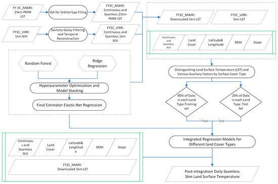
Figure 2.
Flowchart of training the RFRR model and prediction after FY-3C data preprocessing. RFRR refers to the integrated model of Random Forest and Ridge Regression.
- The filling of Orbital Gaps in FY-3C MWRI and PMW data for 25 km surface temperature using Singular Spectrum Analysis.
- Temporal filtering and the daily reconstruction of FY-3C VIRR, using NVI 1 km resolution data based on the Savitzky–Golay method.
- The downscaling of FY-3C MWRI and PMW 25 km resolution surface temperature data using the machine learning RFRR algorithm.
- Training and optimizing the RFRR model to merge FY-3C MWRI and VIRR LST data for different land cover types.
- Generating seamless daily FY-3C 1 km resolution surface temperature data based on the land cover-specific fusion models.
3.1. Singular Value Decomposition Spectrum Analysis (SSA)
In this study, due to the varying positions of missing values in the images on different dates, traditional interpolation methods may not be effectively applied. Therefore, we adopted Singular Spectrum Analysis (SSA) to address the missing values caused by orbital coverage in the FY-3C MWRI PMW data. SSA is an advanced time-series analysis method widely used in remote sensing data processing and analysis. The basic principle of SSA is to decompose the time series into a series of components, including trends, periodic components, and noise, in order to reveal the intrinsic structure and dynamic characteristics of the data. This method helps to improve data quality, fill missing values, and enhance the accuracy of data analysis by extracting the main components of the time series. The processing steps of SSA can be summarized in four key stages:
- (1)
- Embedding: The time series is constructed into a trajectory matrix to facilitate the analysis of its intrinsic structure. For a given time series (xi), this step constructs a trajectory matrix (X) by selecting a window length (L).
- (2)
- Singular Value Decomposition (SVD): SVD occurs on the trajectory matrix (X), decomposing it into the product of three matrices, as follows:where U and V are orthogonal matrices, and ∑ is a diagonal matrix containing the singular values.
- (3)
- Reconstruction: Based on the magnitude of the singular values, select certain singular values and their corresponding singular vectors to reconstruct the time series, separating the main components of the time series. The formula is as follows:where X′ is the matrix reconstructed based on the selected singular value k, Uk, ∑k, and VkT are matrices composed of the selected singular vectors and singular values from the original singular value decomposition. By selecting different k values, various components of the time series (such as trends or periodic components) can be extracted.
- (4)
- Diagonal Averaging: perform diagonal averaging on the reconstructed trajectory matrix to convert it back into the time-series format.
When processing global microwave images, we first treat the surface temperature data in each image as a time series and apply the SSA method to decompose and reconstruct these time series. Considering that the missing values in microwave images appear in long strips and their positions vary by date, we analyze the surface temperature data of each day as a separate time series. For each time series, we select an appropriate window length T to construct the trajectory matrix X. After applying Singular Value Decomposition (SVD) to the trajectory matrix, we classify the components into signal and noise parts based on the magnitude of the singular values, with the signal part typically corresponding to the larger singular values. We then reconstruct the signal components and use diagonal averaging to restore the time series. The reconstructed time series is used to fill in the missing values in the original data, as shown in Figure 3 and Figure 4.
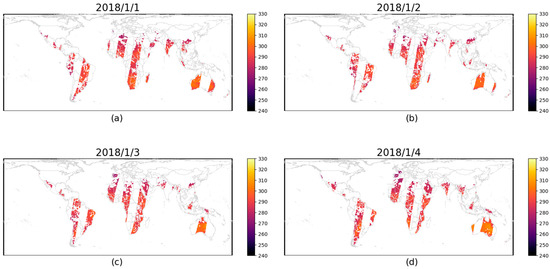
Figure 3.
The map of original FY3C PMW-LST on (a) 1 January 2018, (b) 2 January 2018, (c) 3 January 2018, and (d) 4 January 2018.
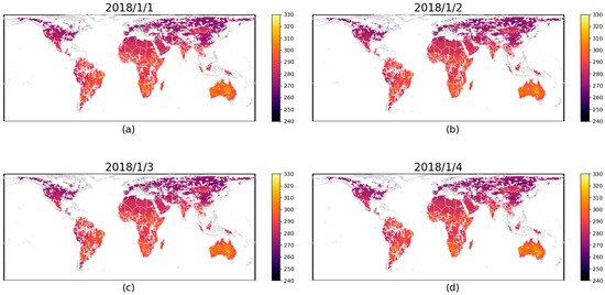
Figure 4.
The map of PMW-LST after Singular Spectrum Analysis reconstruction on (a) 1 January 2018, (b) 2 January 2018, (c) 3 January 2018, and (d) 4 January 2018.
3.2. Savitzky–Golay Filter (S-G Filter)
The Savitzky–Golay filter (S-G filter) is a technique used for data smoothing, which smooths the data by fitting a polynomial to the original signal. Compared to other smoothing methods, the S-G filter better preserves the characteristics of the data, such as peaks and widths. It is widely used in fields such as chemistry, spectroscopy, and signal processing, and is particularly effective for smoothing noisy data. The S-G filter can effectively remove random noise while retaining the important characteristics of the signal.
The essence of the S-G filter is to fit a subset of data points to a low-order polynomial and then use the values of this polynomial to replace the original data points. First, the size of the sliding window (usually an odd number to ensure a central point) and the degree of the polynomial are determined. The window size dictates the number of data points used for each fitting, while the polynomial degree determines the complexity of the fitting.
where n is the order of the polynomial, and a0, a1, a2 …an are the coefficients of the polynomial. These coefficients are calculated by minimizing the sum of squared errors given by the following formula:
where m is the window radius ((window size − 1)/2), yi is the value of the data point within the window, and xi is the corresponding independent variable value.
By solving this least squares problem, we can obtain the polynomial coefficients and then use this polynomial to calculate the new data point value at the center of the window. This process is repeated for all data points, ultimately resulting in a smoothed data sequence.
Applying the Savitzky–Golay filter, the decadal NDVI images are converted into continuous, seamless, and smooth image sequences through local polynomial fitting. In this process, the window size is set to 11 and the polynomial order to 2, to minimize the sum of squared errors at each time point and generate new smooth NDVI values. By selecting an appropriate window size and polynomial order, this method effectively smooths out random fluctuations in the original data while preserving key trends in ecological and environmental changes. This technique not only improves the visual quality of the images but also provides a finer and more continuous dynamic of vegetation cover in the temporal dimension, enhancing the capability for monitoring and analyzing vegetation changes.
3.3. Microwave Data Downscaling
3.3.1. Feature Vector Generation for LST Conversion
To transform MWRI LST data from 25 km to 1 km resolution, we used a statistical downscaling approach that integrates auxiliary predictors at finer resolutions. The key predictors used in this process are the Normalized Difference Vegetation Index (NDVI), the digital elevation model (DEM), and slope data. These predictors are associated with the MWRI LST data, and their relationship is captured using regression models. Below is the procedure followed:
- Data Preparation: The original LST data at 25 km resolution is complemented by auxiliary features such as NDVI, DEM, and slope, each of which is provided at a 1 km resolution. These predictor datasets are loaded from respective directories and combined to form a feature vector for each LST data point. The NDVI, DEM, and slope are critical in capturing the variations in surface characteristics that influence LST.
- Regression Models: Using the downscaled predictor datasets (NDVI, DEM, and slope), regression models are constructed for each LST band. These models represent the relationship between the downscaled predictors and the LST values. The downscaled LST (DLST) data are obtained by applying these models to the predictor feature vectors.
- Data Fusion: The downscaled LST values are combined with the fine-resolution predictors (NDVI, DEM, and slope), creating a fused dataset at 1 km resolution. This allows the higher-resolution spatial information to be incorporated into the downscaled LST data.
These features are combined using statistical regression methods to predict the LST at the finer 1 km resolution. The entire process of downscaling includes multiple regression models for each LST band, with models being discarded if they fail to meet a specified R2 threshold (default set at 0.3) or if more than 40% of their pixels are missing.
3.3.2. Residual Variability (Variogram) Analysis
Variogram analysis is a crucial tool to assess spatial variability in geospatial datasets. For this study, we analyzed the residual variability before and after downscaling to quantify the effectiveness of the downscaling procedure.
- Residual Calculation: After applying the regression models for downscaling, the residuals are calculated by subtracting the predicted DLST values from the original LST values at a 25 km resolution. With residual correction enabled, the residuals are further refined and added back to the downscaled LST values to correct for any spatial discrepancies.where ri represents the residuals, LSTi is the original LST value, and DLSTi is the predicted downscaled LST value.
- Variogram Construction: A variogram is computed for the residuals both before and after the residual correction. The variogram quantifies the spatial autocorrelation of the residuals by measuring how the differences between values change as a function of the distance between them. A typical variogram is constructed using the following formula:where γ(h) is the semivariance at lag distance h, Z(xi) and Z(xj) are the values at locations xi and xj, and N(h) is the number of pairs of data points separated by the distance h.
- Pre- and Post-Correction Variogram: The variogram is computed for the residuals both before and after the residual correction step. This provides insight into how the spatial variability of the residuals is reduced after the correction, thus allowing for a more accurate representation of the spatial pattern in the downscaled LST data. The analysis of the variogram enables us to assess the spatial structure and effectiveness of the downscaling process in reducing residuals.
By combining regression-based downscaling with residual correction and variogram analysis, this approach provides a robust method for enhancing the spatial resolution of MWRI LST data and ensuring that the downscaled data retains its spatial integrity and accuracy.
3.4. Random Forest and Ridge Regression Ensemble Algorithm (RFRR)
3.4.1. Random Forest (RF)
Random Forest is a machine learning method that makes predictions by constructing multiple decision trees. Its key feature is that each tree is built by randomly selecting a subset of features, which helps to reduce the model’s variance and improve its generalization ability. Random Forest performs well in handling large datasets and problems with complex data structures. Additionally, it is effective in dealing with missing values and outliers.
The working principle of Random Forest is to first extract multiple sample sets from the original dataset using bootstrap sampling (sampling with replacement). Then, a decision tree is built for each sample set. During the construction of each decision tree, only the best feature from a randomly selected subset of features is considered when splitting each node. Finally, the Random Forest prediction result is obtained by voting on the results of all decision trees (for classification problems) or averaging them (for regression problems). Given the complex relationships between surface temperature and numerous environmental variables, the Random Forest algorithm can effectively handle missing values and outliers while performing the nonlinear mapping of data features.
When using the Random Forest algorithm for model training, it is essential to configure the software environment and training parameters properly. In this study, the Random Forest machine learning library was used to construct the model within the software environment of the Windows 11, PyCharm 2023.2.1 Integrated Development Environment (IDE), and Python 3.11.5. Table 3 lists the main hyperparameters of the Random Forest model, while the other parameters not listed were set to their default values.
Table 3.
Table of hyperparameters for Random Forest used in stacking.
Due to the large-scale 1 km product over 1062 days, a substantial number of RF evaluations are required, leading to high computational demands. As a result, multiple experiments were conducted to determine the optimal selection of n_estimators. Ultimately, a value of 10 was chosen for the experiment, as this setting mitigates the risk of memory overflow, while maintaining a similar level of accuracy compared to larger models. Moreover, this configuration significantly improved operational efficiency. The following Table 4 outlines the hardware specifications.
Table 4.
Table of hardware specifications.
Under these hardware conditions, the model training time per year is approximately 9 h.
3.4.2. Ridge Regression
Ridge regression is an improved linear regression method used to handle datasets with multicollinearity (high correlation among the input variables). It reduces model complexity and prevents overfitting by adding an L2 norm penalty term (regularization term) to the loss function.
The key feature of ridge regression lies in the introduction of the regularization term. The regularization term is the sum of the squares of the model coefficients, multiplied by a regularization parameter (λ). Adding the regularization term helps make the model coefficients smoother, and in the presence of multicollinearity, it effectively reduces the model’s sensitivity to noise and improves its generalization ability. Given the potential strong correlation between multiple environmental factors, ridge regression stabilizes the estimation of these variables, enhancing the model’s robustness while preventing overfitting.
In the chlorophyll concentration model based on ridge regression in the experiment by Y. Lin and C. Lin [24], ridge regression significantly improved the model’s stability. However, due to the difficulty of ridge regression in handling complex relationships between data features and target variables, no improvement was observed in the estimation of CHLS for water-stressed leaves. Therefore, it is necessary to complement and stack ridge regression with the Random Forest algorithm.
The software environment for the ridge regression algorithm is the same as that for the Random Forest algorithm mentioned above. Table 5 lists the main hyperparameters of the ridge regression model, while the other parameters not listed were set to their default values.
Table 5.
Table of hyperparameters for ridge regression used in stacking.
3.4.3. Ensemble Algorithm
Ensemble algorithms are a machine learning paradigm that improve prediction accuracy and robustness by combining multiple models. In this approach, several different models are trained and applied to the same task, with the final output typically combined in some way (such as averaging or voting) with the individual model results. Random Forest, as a key component of ensemble learning, excels in classification and regression tasks, particularly when dealing with data that have complex structures and high-dimensional features. It improves prediction accuracy and generalization ability by constructing multiple decision trees and aggregating their predictions. Ridge regression, as another key component, robustly handles highly correlated features through the L2 regularization mechanism, effectively preventing overfitting, especially when the number of features exceeds the number of samples.
This ensemble algorithm typically involves combining the prediction results of Random Forest and Ridge Regression. The combination method can be simple, such as averaging, weighted averaging, or more complex techniques like stacking. In the stacking method, the prediction results of Random Forest and Ridge Regression are used as inputs for another model to learn and optimize the best way to combine these predictions.
3.4.4. Continuous All-Weather TIR Land Surface Temperature
The ensemble algorithm of Random Forest and Ridge Regression (RFRR) has a strong ability to fit complex nonlinear relationships, making it an ideal choice for developing a continuous all-weather TIR LST generation model. The fundamental premise for constructing such a model is that the nonlinear relationship between LST and other environmental variables remains consistent under both clear and cloudy conditions. Based on this premise, this study utilizes the RFRR algorithm to establish a nonlinear relationship model between FY-3C VIRR LST and six environmental variables (Downscaled PMW LST, NVI, LC, longitude and latitude, slope, and DEM) under clear conditions. Subsequently, the RFRR model established under clear conditions is applied to all-weather conditions to generate spatially continuous LST products, referred to as RFRR LST (RFRR-LST). Finally, RFRR-LST is used to fill the cloudy pixels of FY-3C VIRR LST, generating an all-weather LST product, called the Filled FY-3C VIRR LST (FM-LST).
To present the proposed all-weather LST generation method in a more structured manner, it is divided into three main steps:
- Selection of Input Variables for the RFRR Model:
Surface temperature is influenced by numerous environmental variables. In this study, the input variables for the RFRR model include Dow_LST, NDVI, LC, DEM, slope, and climate. Dow_LST refers to the microwave data that has been filled using SSA and downscaled. The NDVI has been normalized and smoothed using the S-G filter. It is important to note that different land cover types exhibit distinct surface temperature characteristics. For instance, the surface temperature of bare soil is higher than that of vegetation during the day, but lower at night. Therefore, this study selects NDVI and LC as input variables.
China’s climate exhibits significant latitudinal and land–sea heterogeneity, leading to variations in surface temperature driven by different climate types. Additionally, surface temperature is also influenced by DEM and slope. As a result, longitude and latitude, DEM, and slope data are chosen as input variables for the RFRR model.
- 2.
- Establishment of the RFRR Model for Generating Continuous All-Weather TIR Land Surface Temperature:
Leveraging the powerful nonlinear fitting capability of the RFRR algorithm, this study proposes a continuous all-weather LST generation method, which includes two key steps. First, using monthly time-series datasets, an RFRR model is trained and established to represent the relationship between FY-3C VIRR LST and six environmental variables (Downscaled PMW LST, NDVI, LC, longitude and latitude, slope, and DEM) under clear conditions. During model training, the dataset is split into training and testing sets in an 80:20 ratio. The training dataset is used to train the RFRR model, while the testing dataset is used to prevent overfitting. Next, the RFRR model established under clear conditions is applied to all-weather conditions. By inputting the six environmental variables for date T into the trained RFRR model, a high-resolution and spatially continuous LST for date T is generated, referred to as RFRR-LST.
- 3.
- Generation of All-Weather LST:
Due to its high spatial resolution and retrieval accuracy, TIR LST is often used for generating all-weather LST. FY-3C LST is one of the most commonly used TIR LST datasets in China. Therefore, this study uses the FY-3C Level 3 LST product, VIRR LST, as the base data for generating all-weather LST. To generate all-weather LST, we fill the cloudy pixels in VIRR LST with RFRR-LST values generated by the RFRR model. Specifically, each cloudy pixel in VIRR LST is identified and subsequently replaced with the corresponding RFRR-LST value, thereby generating an all-weather LST derived from a VIRR LST. This newly generated all-weather LST is denoted as FMLST (Fusion Microwave Land Surface Temperature).
3.5. Validation Metrics
The performance of the generated all-weather LST was evaluated using validation metrics such as Mean Absolute Error (MAE), Root Mean Square Error (RMSE), and the Coefficient of Determination (R2). These metrics are defined as follows:
In these formulas, n represents the number of observations; yi and represent the observed values and the estimated values, respectively; and denotes the mean of the actual observed values.
4. Results
4.1. Annual Variation Analysis of Model Accuracy at Different Sites
By comparing and analyzing the fused surface temperature (FM-LST) data from 2017 to 2019 with the in situ measured surface temperature (Site LST) at each station, the impact of different surface types on model accuracy can be observed, as shown in Figure 5, Figure 6 and Figure 7. The data for each year exhibit some fluctuation, but overall, the model successfully captures the seasonal variation trend of surface temperature.
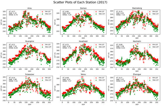
Figure 5.
Scatter plot comparison of LST reconstructed using the RFRR machine learning model in 2017 with LST measured by AWS at 8 sites. FM-LST represents the fused LST predicted by the model; Site-LST represents the LST measured by the observation station.
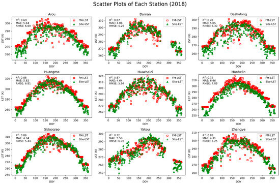
Figure 6.
Scatter plot comparison of LST reconstructed using the RFRR machine learning model in 2018 with LST measured by AWS at 8 sites. FM-LST represents the fused LST predicted by the model; Site-LST represents the LST measured by the observation station.
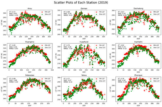
Figure 7.
Scatter plot comparison of LST reconstructed using the RFRR machine learning model in 2019 with LST measured by AWS at 8 sites. FM-LST represents the fused LST predicted by the model; Site-LST represents the LST measured by the observation station.
In the 2019 data, the Sidaoqiao station exhibited the best prediction accuracy (R2 = 0.89), indicating that the model performs with high reliability in predicting surface temperature in this region. This result is likely related to the region’s geographical features and relatively uniform land cover types, such as poplar forests, which provide favorable environmental conditions, allowing the model to predict surface temperature more accurately.
For some stations with lower prediction accuracy, such as the Dashalong station, the 2019 data showed an R2 of 0.67, indicating relatively lower accuracy. The Dashalong station is located in an alpine meadow, where surface types may be influenced by elevation heterogeneity and seasonal variations in cover, potentially affecting the model’s accuracy. Additionally, changes in cloud cover may also impact the quality of thermal infrared data, further influencing the prediction accuracy of FMLST.
When comparing data from the three years, it was found that the R2 values for most stations remained above 0.70, indicating that the model was consistently able to capture the trend of surface temperature changes. Although some stations, such as Huazhaizi, showed slightly lower R2 values in certain years, this phenomenon may be related to the unique topography and climate conditions of the desert area where the station is located. In this environment, surface temperature is influenced by multiple factors, such as wind erosion, and significant variations in surface moisture, which may lead to substantial discrepancies between the measured values and the model predictions.
The experimental results show that the model can effectively predict surface temperature under various surface conditions. Although there is some fluctuation in prediction accuracy at certain sites with complex topography, the model overall successfully captures the dynamic trend of surface temperature changes over time. This demonstrates the significant potential of machine learning methods in the analysis of surface temperature remote sensing data and provides a feasible solution for accurate remote sensing monitoring under complex cloud cover conditions.
4.2. Accuracy Validation for Different Land Cover Types
By analyzing the accuracy validation bar charts classified by six different land cover types for the years 2017, 2018, and 2019 (as shown in Figure 8), several key trends and insights can be revealed.
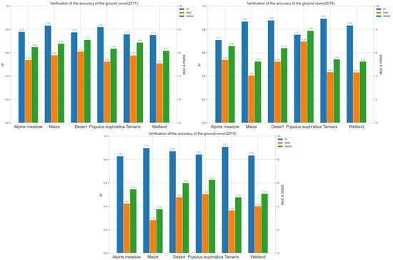
Figure 8.
Bar chart of validation accuracy metrics (R2, MAE, RMSE) of FM-LST for different land cover types from 2017 to 2019.
In the 2017 data, the R2 value for the desert areas was the highest, while the R2 value for the alpine meadows was the lowest. This result may indicate that the model’s surface temperature prediction capability is superior for land cover types such as deserts, which could be due to the relatively uniform surface characteristics and lower vegetation coverage in desert regions. In the same year, the MAE and RMSE values for the corn regions were higher, suggesting that surface temperature prediction for this land cover type was more challenging, or there were factors not fully captured by the model.
In 2018, the model’s prediction accuracy improved across all land cover types, especially in the desert and marshland types, where the R2 values reached 0.88 and 0.83, respectively, demonstrating the model’s robustness and good adaptability to these surface types. Additionally, the prediction accuracy for the corn regions also significantly improved, with notable reductions in the MAE and RMSE values.
In 2019, the model achieved the highest prediction accuracy for the wetland areas (R2 = 0.91), while the R2 value for the desert regions showed a slight decrease but still remained at a high level (R2 = 0.85). In this year, the MAE and RMSE values for all land cover types were generally lower than those in 2017, indicating that the accuracy and reliability of the model’s predictions have improved year by year.
In summary, the model demonstrates robust predictive performance across different land cover types, with particularly significant improvements in prediction accuracy for marshland and desert environments. This result proves the model’s high capability in capturing surface temperature variations, providing a reliable technical approach for surface temperature monitoring. Although prediction accuracy shows some fluctuation in certain specific land cover types, the overall trend indicates continuous improvement, further validating the feasibility and rationality of the FM-LST generation method proposed in this study.
4.3. Site Accuracy Validation
Figure 9 presents a comparative analysis of the surface temperature data from microwave, thermal infrared, and FMLST images for the years 2017 to 2019. These datasets were validated against site-measured data, revealing their respective performance in surface temperature estimation.
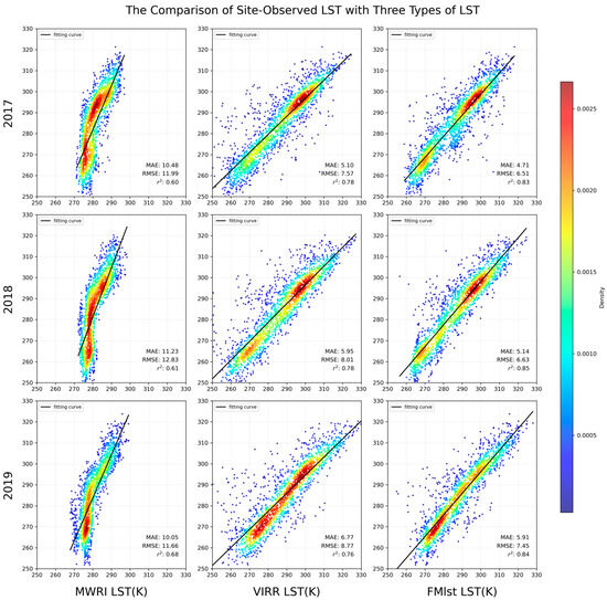
Figure 9.
Validation density scatter plot of site-observed LST compared with three types of LST—MWRIX LST, VIRR LST, and FM LST from 2017 to 2019.
The scatter plots comparing the microwave data with site data show relatively low R2 values and higher MAE and RMSE values across the 2017 to 2019 validations, consistent with the lower original resolution of the microwave data. While thermal infrared data was affected by cloud cover, it exhibited higher accuracy in cloud-free conditions, with generally higher R2 values, indicating its direct effectiveness in surface temperature estimation.
Building on this, the fused FMLST data, combined through stacked machine learning techniques, demonstrated the best accuracy performance across all three years of validation. Taking the 2019 data as an example, the R2 value for FMLST reached 0.85, with MAE reduced to 4.71 K and RMSE reduced to 6.51 K. The dense clustering of data points in the density scatter plot highlights the significant effect of FMLST in filling cloud-covered areas and improving surface temperature estimation accuracy.
Overall, the three years of validation results indicate that the FMLST model can effectively improve surface temperature prediction accuracy, particularly under complex cloud cover conditions. This finding underscores the importance of integrating different remote sensing data sources and provides empirical support for future applications in related fields.
4.4. Spatial Layout and Difference Comparison Between FMLST and MODIS-LST
In this study, we employed an innovative method to generate fused surface temperature (LST) data, which relies solely on observations from the Fengyun-3C satellite (FY-3C) without using MODIS LST data. By carefully selecting days with minimal cloud cover each month for LST image generation and validation, we ensured that the annual density scatter plots included a large number of valid comparison points, providing sufficient data support for an error analysis. Despite this strategy, the original MODIS images still exhibited significant cloud contamination and blank areas, which contrast sharply with the completeness of the fused images, as shown in Figure 10, Figure 11 and Figure 12.
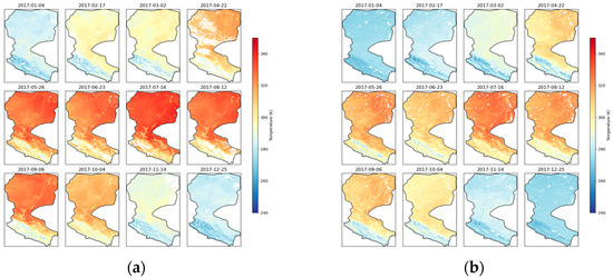
Figure 10.
Spatial layout comparison of 2017 (a) MODIS and (b) FMLST.
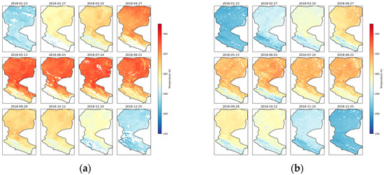
Figure 11.
Spatial layout comparison of 2018 (a) MODIS and (b) FMLST.
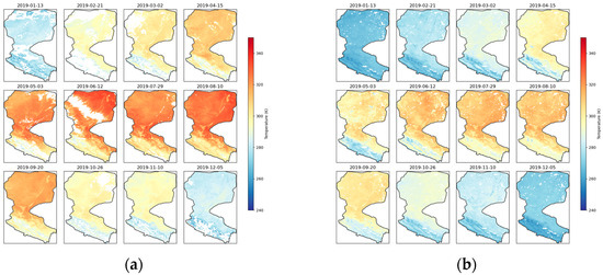
Figure 12.
Spatial layout comparison of 2019 (a) MODIS and (b) FMLST.
In the comparison of the three consecutive years from 2017 to 2019, the FM-LST images demonstrated excellent spatial continuity and completeness, particularly during the spring and summer seasons when the surface was covered by clouds. In these conditions, the FM-LST images provided a more coherent and detailed distribution of surface temperature, which could not be achieved in the MODIS images due to data gaps caused by cloud cover.
For the autumn months with fewer clouds, both the FM-LST and MODIS images displayed richer and more consistent surface temperature information. However, the FM-LST images exhibited smoother temperature transitions and fewer data anomalies in some details, reflecting the advantages of the fusion algorithm in handling boundaries and temperature gradients.
Further analysis, as shown in Figure 13, clearly demonstrates the high correlation between the FM-LST and MODIS LST data in the annual density scatter plots, which is particularly significant in the large sample datasets (1,666,037 valid points in 2017, 1,652,949 in 2018, and 1,578,885 in 2019). Statistical error parameters, particularly the coefficient of determination (r2 = 0.88) for the 2019 data, reveal a strong positive correlation between the two data sources.
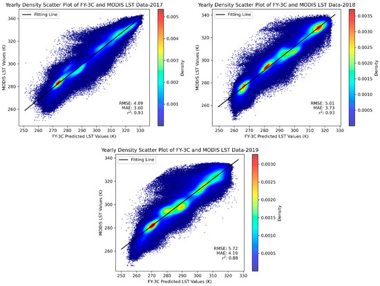
Figure 13.
The 2017–2019 Annual Density Scatter Plots for MODIS and FMLST.
Although the RMSE for 2019 showed a slight increase, this may be due to systematic errors introduced by cloud cover or other environmental factors. Furthermore, the areas with the highest density in the scatter plots, typically represented by the brightest colors, closely align with the best fit line. This further emphasizes that, in these large sample datasets, the consistency between the fused data and the MODIS data is higher than the overall trend.
These results not only demonstrate that our fusion technology can provide continuous and consistent data in cloud-covered areas, but also highlight its potential to generate high-precision surface temperature information under various meteorological conditions. The large number of valid data points provides a solid foundation for our error analysis, enhancing the credibility and persuasiveness of the experimental results.
5. Discuss
To address the issue of data loss in FY-3C VIRR data due to cloud cover, this study developed an LST-filling method based on a Random Forest (RF) and Ridge Regression (RR) algorithm stacking model, which relies entirely on Fengyun FY-3C data. This method combines FY-3C MWRI data and FY-3C VIRR’s NVI data, using Singular Spectrum Analysis (SSA) to fill missing orbital data and performing time reconstruction with Savitzky–Golay filtering to obtain continuous, seamless NDVI data. Further, the PMW LST data from FY-3C MWRI and the NDVI data are used to downscale the surface temperature, resulting in higher-resolution 1 km LST data. The stacked Random Forest and Ridge Regression machine learning algorithms are employed to model the relationships between various environmental variables and surface temperature. These environmental variables include continuous, seamless NDVI, land cover (LC), longitude, latitude, digital elevation model (DEM), and slope. By optimizing the model’s hyperparameters and applying stacking (Model Stacking), Elastic Net Regression was selected as the final regression model. The data for different land cover types were integrated to train the regression model. After model training and testing, the data for the target date are used to generate a 1 km surface temperature product (FM-LST) under all-weather conditions, ultimately producing a daily continuous, seamless 1 km surface temperature product.
In this study, daily noon time series data from 2017 to 2019 were used to build 36 RFRR stacking models (12 × 3) on a monthly basis. In the presence of missing data, 1062 FM-LST products were generated (350 + 352 + 360). To analyze the feature importance of the RFRR stacking model from 2017 to 2019, a SHAP value analysis was conducted, as shown in Figure 14. The results indicated that Dow_LST is the dominant feature in the model, particularly in 2018 and 2019. The SHAP value of Dow_LST was significantly higher than the other variables, and its positive impact showed a yearly increasing trend. This result aligns with the key role of Dow_LST in the microwave data downscaling product, further validating its importance for the accuracy of surface temperature prediction under cloud cover conditions.
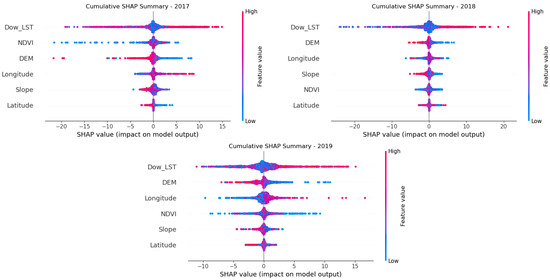
Figure 14.
SHAP-based feature importance analysis of the RFRR model from 2017 to 2019.
Specifically, the average SHAP value of Dow_LST in 2019 was around 10, significantly higher than 5 in 2017 and 8 in 2018, indicating that its influence on the model increased year by year. The impact of the DEM and NDVI remained relatively stable, with average SHAP values fluctuating between three and five. In contrast, geographically related features—latitude and longitude—contributed less to the model. For the NDVI, the average SHAP value in 2017 was around four, dropping to about two in 2018, which may reflect changes in climate conditions or vegetation growth patterns that year. By 2019, the influence of the NDVI had slightly increased. The DEM showed relatively consistent influence over the analysis period.
Overall, Dow_LST made a significant contribution to the model, especially in addressing cloud cover issues. Moreover, the findings highlight the importance of integrating topographical, vegetation, and geographical information for surface temperature prediction.
6. Conclusions
This study concludes the following:
- Based on FY-3C satellite data and auxiliary environmental variables, and by employing machine learning methods (RFRR stacking model), this study successfully generated 1062 days of all-weather surface temperature (FM-LST) from 2017 to 2019. An analysis showed that Dow_LST in the microwave data downscaling product, as the dominant feature in the model, increased in importance over the years and significantly impacted the prediction accuracy of surface temperature under cloud cover conditions. Other environmental variables, such as the DEM and NDVI, while showing stable influence, played a relatively smaller role in surface temperature prediction.
- Through a comparative analysis of FM-LST with in situ site measurements of surface temperature, it was found that different land cover types affected the model’s accuracy. Over several years of data, the model reflected the seasonal variation of surface temperature. Although there was some fluctuation in prediction accuracy for certain land cover types, the model’s prediction accuracy was high at most sites, demonstrating the effectiveness of the method. This trend was reflected in the accuracy validation bar charts for the different land cover types, with particularly significant prediction accuracy in the marshland and desert environments.
Compared to previous studies, this research is the first to fully rely on Fengyun satellite series data, including vegetation index, infrared, and microwave temperature, to achieve a comprehensive reconstruction of surface temperature. Through precise machine learning techniques, we successfully filled the data gaps caused by cloud cover, enhancing the accuracy and reliability of surface temperature estimation. This pioneering work not only improves the spatial continuity of surface temperature data but also establishes a solid foundation for the application of Fengyun satellite series data in surface temperature monitoring.
Author Contributions
X.L. contributed to searching the literature, describing the model, analyzing the data and model performances, providing the figures and maps, and writing the manuscript. W.Z. and Q.Z. contributed to designing the research. T.S. and Z.C. contributed to remote sensing data processing. All authors have read and agreed to the published version of the manuscript.
Funding
This research was funded by the National Key Research and Development Program of China (2022YFE0113900) and the National Natural Science Foundation of China (Grant No. 42301420).
Institutional Review Board Statement
Not applicable.
Informed Consent Statement
Not applicable.
Data Availability Statement
Data presented in this research are available upon fair request.
Acknowledgments
The remote sensing data for this experiment were provided by the Fengyun Satellite Meteorological Innovation Center (FYSIC), and the site validation data were sourced from the Third Pole Environment Data Center (TPDC) (http://data.tpdc.ac.cn, accessed on 27 March 2024). We sincerely thank the FYSIC and the TPDC for their support in providing the data.
Conflicts of Interest
The authors declare no conflicts of interest.
References
- Anderson, M.C.; Norman, J.M.; Kustas, W.P.; Houborg, R.; Starks, P.J.; Agam, N. A Thermal-Based Remote Sensing Technique for Routine Mapping of Land-Surface Carbon, Water and Energy Fluxes from Field to Regional Scales. Remote Sens. Environ. 2008, 112, 4227–4241. [Google Scholar] [CrossRef]
- Kalma, J.D.; McVicar, T.R.; McCabe, M.F. Estimating Land Surface Evaporation: A Review of Methods Using Remotely Sensed Surface Temperature Data. Surv. Geophys. 2008, 29, 421–469. [Google Scholar] [CrossRef]
- Li, Z.-L.; Tang, B.-H.; Wu, H.; Ren, H.; Yan, G.; Wan, Z.; Trigo, I.F.; Sobrino, J.A. Satellite-Derived Land Surface Temperature: Current Status and Perspectives. Remote Sens. Environ. 2013, 131, 14–37. [Google Scholar] [CrossRef]
- Zhang, W.; Yu, Q.; Tang, H.; Liu, J.; Wu, W. Conservation Tillage Mapping and Monitoring Using Remote Sensing. Comput. Electron. Agric. 2024, 218, 108705. [Google Scholar] [CrossRef]
- Wan, Z. New Refinements and Validation of the MODIS Land-Surface Temperature/Emissivity Products. Remote Sens. Environ. 2008, 112, 59–74. [Google Scholar] [CrossRef]
- Duan, S.-B.; Li, Z.-L.; Wu, H.; Leng, P.; Gao, M.; Wang, C. Radiance-Based Validation of Land Surface Temperature Products Derived from Collection 6 MODIS Thermal Infrared Data. Int. J. Appl. Earth Obs. Geoinf. 2018, 70, 84–92. [Google Scholar] [CrossRef]
- Liu, Y.; Yu, Y.; Yu, P.; Göttsche, F.; Trigo, I. Quality Assessment of S-NPP VIIRS Land Surface Temperature Product. Remote Sens. 2015, 7, 12215–12241. [Google Scholar] [CrossRef]
- Zhou, J.; Dai, F.; Zhang, X.; Zhao, S.; Li, M. Developing a Temporally Land Cover-Based Look-up Table (TL-LUT) Method for Estimating Land Surface Temperature Based on AMSR-E Data over the Chinese Landmass. Int. J. Appl. Earth Obs. Geoinf. 2015, 34, 35–50. [Google Scholar] [CrossRef]
- Xu, S.; Cheng, J.; Zhang, Q. A Random Forest-Based Data Fusion Method for Obtaining All-Weather Land Surface Temperature with High Spatial Resolution. Remote Sens. 2021, 13, 2211. [Google Scholar] [CrossRef]
- Yu, P.; Zhao, T.; Shi, J.; Ran, Y.; Jia, L.; Ji, D.; Xue, H. Global Spatiotemporally Continuous MODIS Land Surface Temperature Dataset. Sci. Data 2022, 9, 143. [Google Scholar] [CrossRef]
- Xu, S.; Cheng, J.; Zhang, Q. Reconstructing All-Weather Land Surface Temperature Using the Bayesian Maximum Entropy Method Over the Tibetan Plateau and Heihe River Basin. IEEE J. Sel. Top. Appl. Earth Obs. Remote Sens. 2019, 12, 3307–3316. [Google Scholar] [CrossRef]
- Li, Z.-L.; Leng, P. A Framework for the Retrieval of All-Weather Land Surface Temperature at a High Spatial Resolution from Polar-Orbiting Thermal Infrared and Passive Microwave Data. Remote Sens. Environ. 2017, 195, 107–117. [Google Scholar] [CrossRef]
- Sun, D.; Li, Y.; Zhan, X.; Houser, P.; Yang, C.; Chiu, L.; Yang, R. Land Surface Temperature Derivation under All Sky Conditions through Integrating AMSR-E/AMSR-2 and MODIS/GOES Observations. Remote Sens. 2019, 11, 1704. [Google Scholar] [CrossRef]
- Wang, T.; Shi, J.; Yan, G.; Zhao, T.; Ji, D.; Xiong, C. Recovering Land Surface Temperature under Cloudy Skies for Potentially Deriving Surface Emitted Longwave Radiation by Fusing MODIS and AMSR-E Measurements. In Proceedings of the 2014 IEEE Geoscience and Remote Sensing Symposium, Quebec City, QC, Canada, 13–18 July 2014; pp. 1805–1808. [Google Scholar]
- Zhang, X.; Zhou, J.; Gottsche, F.-M.; Zhan, W.; Liu, S.; Cao, R. A Method Based on Temporal Component Decomposition for Estimating 1-Km All-Weather Land Surface Temperature by Merging Satellite Thermal Infrared and Passive Microwave Observations. IEEE Trans. Geosci. Remote Sens. 2019, 57, 4670–4691. [Google Scholar] [CrossRef]
- Stevens, F.R.; Gaughan, A.E.; Linard, C.; Tatem, A.J. Disaggregating Census Data for Population Mapping Using Random Forests with Remotely-Sensed and Ancillary Data. PLoS ONE 2015, 10, e0107042. [Google Scholar] [CrossRef]
- Shwetha, H.R.; Kumar, D.N. Prediction of High Spatio-Temporal Resolution Land Surface Temperature under Cloudy Conditions Using Microwave Vegetation Index and ANN. ISPRS J. Photogramm. Remote Sens. 2016, 117, 40–55. [Google Scholar] [CrossRef]
- Tang, Y.; Zhang, J.; Wang, J. FY-3 Meteorological Satellites and the Applications. Chin. J. Space Sci. 2014, 34, 703. [Google Scholar] [CrossRef]
- Hoerl, A.E.; Kennard, R.W. Ridge Regression: Biased Estimation for Nonorthogonal Problems. Technometrics 2000, 42, 80–86. [Google Scholar] [CrossRef]
- Breiman, L. Random Forests. Mach. Learn. 2001, 45, 5–32. [Google Scholar] [CrossRef]
- Cheng, G.; Li, X.; Zhao, W.; Xu, Z.; Feng, Q.; Xiao, S.; Xiao, H. Integrated Study of the Water–Ecosystem–Economy in the Heihe River Basin. Natl. Sci. Rev. 2014, 1, 413–428. [Google Scholar] [CrossRef]
- Che, T.; Li, X.; Liu, S.; Li, H.; Xu, Z.; Tan, J.; Zhang, Y.; Ren, Z.; Xiao, L.; Deng, J.; et al. Integrated Hydrometeorological—Snow—Frozen Ground Observations in the Alpine Region of the Heihe River Basin, China 2019. Earth Syst. Sci. Data 2019, 11, 1483–1499. [Google Scholar] [CrossRef]
- Liu, S.; Li, X.; Xu, Z.; Che, T.; Xiao, Q.; Ma, M.; Liu, Q.; Jin, R.; Guo, J.; Wang, L.; et al. The Heihe Integrated Observatory Network: A Basin-Scale Land Surface Processes Observatory in China. Vadose Zone J. 2018, 17, 1–21. [Google Scholar] [CrossRef]
- Lin, C.-Y.; Lin, C. Using Ridge Regression Method to Reduce Estimation Uncertainty in Chlorophyll Models Based on Worldview Multispectral Data. In Proceedings of the IGARSS 2019—2019 IEEE International Geoscience and Remote Sensing Symposium, Yokohama, Japan, 28 July–2 August 2019; pp. 1777–1780. [Google Scholar]
Disclaimer/Publisher’s Note: The statements, opinions and data contained in all publications are solely those of the individual author(s) and contributor(s) and not of MDPI and/or the editor(s). MDPI and/or the editor(s) disclaim responsibility for any injury to people or property resulting from any ideas, methods, instructions or products referred to in the content. |
© 2025 by the authors. Licensee MDPI, Basel, Switzerland. This article is an open access article distributed under the terms and conditions of the Creative Commons Attribution (CC BY) license (https://creativecommons.org/licenses/by/4.0/).